Nonlinear Stress Analysis of SMA Beam Based on the Three-dimensional Boyd-Lagoudas Model Considering Large Deformations

(1)

Vol. 2, No. 2, Autumn−Winter 2017-18

Nonlinear Stress Analysis of SMA Beam Based on the

Three-dimensional Boyd-Lagoudas Model Considering

Large Deformations

R. Zamani, M. Botshekanan Dehkordi

∗

Mechanical Engineering Department, Shahrekord University, Shahrekord, Iran.

Article info

Article history:

Received 04 January 2018 Received in revised form 24 February 2018

Accepted 24 February 2018

Keywords: SMA beam

Superelastic bending Boyd-Lagoudas model Timoshenko beam theory Nonlinear FEM

Abstract

In this study, a nonlinear superelastic bending of shape memory alloy (SMA) beam with consideration of the material and geometric nonlinearity effects which are coupled with each other, has been investigated. By using the Timoshenko beam theory and applying the principle of virtual work, the governing equations were extracted. In this regard, Von Karman strains were applied to take the large deflections into account. Via Boyd-Lagoudas 3D constitutive model, SMA was simulated, which was properly reduced to two dimensions. With the development of an iterative nonlinear finite element model, and for the purpose of obtaining characteristic of finite element beam, the Galerkin weighted-residual method was applied. In this study, by considering the different force and support conditions for the SMA beam, their effects on the distribution of martensitic volume fraction (MVF) and stress distribution were investigated. The obtained results indicate that the magnitude of MVF and consequently the level of hysteresis increases, which leads to the reduction of the modulus of elasticity and the strength of the material and therefore the deflection of SMA beam increases consequently. To validate the proposed formulation, the results were compared with other experimental and numerical results and a good agreement was achieved between outcomes.

Nomenclature

G Gibbs free energy bM _{Model parameter}

σij Cauchy stress tensor µ1 Model parameter

εi,j Total strain tensor µ2 Model parameter

ν Poisson’s ratio bA _{Model parameter}

εt_ij Transformation strain tensor Λ Transformation tensor ¯

S Eﬀective compliance tensor σ′ Deviatoric stress tensor

¯

c Eﬀective special heat ¯σ′ Eﬀective stress

ξ Martensitic volume fraction π General thermodynamic force

ρ Density ϕ Transformation function

T Current temperature T0 Reference temperature

f(ξ) Transformation hardening function E Youngs modulus

∗_{Corresponding author: M. Botshekanan Dehkordi (Assistant Professor)}

E-mail address: [email protected] http://dx.doi.org/10.22084/jrstan.2018.15454.1038 ISSN: 2588-2597

(2)

¯

u0 Eﬀective special internal energy at

refer-ence state

¯

s0 Eﬀective special entropy at the reference

state ¯

α Eﬀective thermal expansion coeﬃcient ten-sor

Y Critical value for thermodynamic force to cause transformation

Hmax _{Maximum attainable transformation strain} _εt−r _{Transformation strain at the reversal point}

ε−t−r _{Eﬀective transformation strain at the}

rever-sal point

1. Introduction

As far as smart materials exhibit special properties, they are considered as proper choices for industrial ap-plications in many engineering branches. Among the different types of smart materials, SMAs have unique characteristics such as pseudoelasticity behavior and shape memory effect (SME) [1]. The SME recovers the strain generated in the material through a ther-mal phase transformation process. The pseudoelastic-ity behavior of SMA allows the alloy memory to tol-erate large deflection without causing permanent de-formation. The occurrence of these behaviors results from the phase transformation between the two main phases of material martensite and austenite [2].

One of the main mode of application of structures that are made of memory alloy is bending. Modeling and bending analysis of memory rails have been the subject of several other studies. Based on a finite strain description, Jaber et al. [3] presented a finite element model for SMA 3D-beam. A phenomenological correc-tion model was introduced that was capable of simu-lating some aspects of SMA thermodynamic behavior, such as superelasticity and the one-way SME. In their model, strain and temperature were control variables which eliminate the need for transformation correctors of finite element in the analysis. They compared the obtained results with the experimental results of three-point and four-three-point bending tests. Through the bend-ing application which was adapted for the ambient tem-perature conditions, Mineta et al. [4] investigated an active guide wire. Their proposed micro-actuator had a simple and flexible structure that was made of Ni-Ti SMA with meandering shape and bias coil. Gillet et al. [5] presented a numerical method for predicting the behavior of SMA beam in the three-point bending test. The result of their conducted experiments was presented on Cu-based alloys to validate their numer-ical results. Baghani et al. [6] proposed an analyti-cal solution for shape memory polymer (SMP) Euler-Bernoulli beam under bending. Further, in different steps of an SMP cycle, they presented closed form ex-pressions for internal variable variations, stresses, and beam curvature distribution. In another study, Mirza-eifar et al. [7] studied on superelastic bending of SMA beams. Two different transformation functions were considered: J2-based model andJ2−J1-based model.

Closed form expressions were used to analyze the stress and MVF in the cross-section. They obtained the

an-alytical form of the bending moment-curvature rela-tion. Botshekanan et al. [8] presented a Non-linear dynamic analysis of a sandwich beam with pseudoelas-tic SMA hybrid composite faces based on higher order ﬁnite element theory. In their research, the changes of the MVF and the properties of materials in diﬀerent points of the structure were considered continuously. To solve the equations, an iteration method based on transient nonlinear FEM formulation with a dynamic phase transformation algorithm was presented. In ad-dition, to simulate SMA behavior, the Brinson one-dimensional model was applied.

Since the SMA properties are function of stress, it can be therefore said that the properties of SMA beam are variable in different points of the beam; hence, in many studies, simplifications are applied. For exam-ple, a continuous SMA beam was simulated with a one-degree freedom model. In the present research, first for the modeling of nonlinear behavior of SMA beam, it was modeled continuously, and second, multi-dimensional models were used. This study used the Timoshenko beam theory which is a two-dimensional model for beam modeling. Moreover, the nonlinear strain field was used. Furthermore, SMA was applied for the simulation via Boyd-Lagoudas 3D constitutive model, which was properly reduced to two dimensions. In this research, new analyses for SMA beam with dif-ferent support and force conditions were performed, and new results were presented in terms of distribu-tion of stress, distribudistribu-tion of MVF, and displacements of the beam.

2. Modeling of Shape Memory Alloy

In this study, the constitutive model for SMAs pro-posed by Lagoudas [2] was used. This model is de-scribed on the basis of Gibbs free energy. The total Gibbs free energy is obtained through the following equation:

G(σij :T :ξ:εtij) =−

1 ρ 1

2σ: ¯S:σ− 1

ρσ: [ ¯α(T−T0)] + ¯c

[

(T−T0)−Tln

( T T0

)]

−s¯0T+ ¯u0+f(ξ) (1)

whereσij,εtij,ξ,ρ,T, andT0are Cauchy stress tensor,

(3)

represen-tative of the material parameters, which are effective compliance tensor, effective thermal expansion tensor, effective special heat, effective special entropy at the reference state and effective special internal energy at reference state, respectively. Those are expressed as:

¯

S(ξ) =SA+ξ(SM−SA) =SA+ξ∆S

¯

α(ξ) =αA+ξ(αM −αA) =αA+ξ∆α

¯

c(ξ) =cA+ξ(cM−cA) =αA+ξ∆α (2)

¯

s0(ξ) =sA0 +ξ(sM0 −sA0) =sA0 +ξ∆s0

¯

u0(ξ) =uA0 +ξ(u

M

0 −u

A

0) =u

A

0 +ξ∆u0

where the superscripts A and M represent the austenitic and martensitic phases, respectively.

Functionf(ξ) is the transformation hardening func-tion, which is used to consider the interactions be-tween the austenite and martensitic phase, and the ex-isting interactions in the martensitic phase itself. A second-order polynomial form of this function for for-ward transformation ˙ξ <0 and reverse transformation can be introduced as:

f(ξ) =       

ρ 2b

M_ξ2_{+ (µ}

1+µ2)ξ ξ >˙ 0

ρ 2b

A_ξ2_{+ (µ}

1+µ2)ξ ξ <˙ 0

(3)

bM_, _bA_, _µ

1, and µ2 are model parameters which are

achieved through the following forms:

bM =−∆s0(Ms−Mf)

bA=−∆s0(Af−As)

µ1=

1

2ρ∆s0(Ms+Af)−ρ∆u0 µ2=

1

4ρ∆s0(As−Af−Mf +Ms)−ρ∆u0

(4)

where Ms, Mf, As, and Af are martensitic start,

martensitic ﬁnish, austenitic start and austenitic ﬁn-ish temperature, respectively.

Entropy and strain relations are obtained as fol-lows:

s=−∂G ∂T

ε=−ρ∂G ∂σ

(5)

By substituting Eq. (5) into Eq. (1), the entropy and strain relations can be rewritten as below:

s= 1

ρσ:α+cln (

T T0

) +s0

ε=S:σ+α(T−T0) +εt

(6)

According to Eq. (6), stress tensor is given by:

σ=S−1: [ε−α(T−T0)−εt] (7)

The relation between the evolution of the transforma-tion strain and the evolutransforma-tion of martensitic volume fraction during the forward and reverse transformation, which is called the ﬂow rule, can be postulated as:

˙

εt= Λ ˙ξ (8)

where Λ is the transformation tensor and is assumed in the following form:

Λ =         

3 2H

maxσ′

¯ σ′

˙ ξ >0

Hmax ε

t₋r

ε−t−r ξ <˙ 0

(9)

whereHmax_,_σ′_{, ¯}_σ′_,_εt−r_{, and}_ε−t−r _{are maximum}

at-tainable transformation strain, deviatoric stress tensor, eﬀective stress, transformation strain at the reversal point and eﬀective transformation strain at the rever-sal point, respectively.

πis the general thermodynamic force which is ex-pressed as:

π(σ, T, ξ) =σ: Λ +1

2σ: ∆S:σ+σ: ∆σ(T−T0) −ρ∆c

[

(T−T0)−Tln

( T T0

)]

+ρ∆S0T−ρ∆u0−

∂f

∂ξ (10)

The critical values of the thermodynamic force for for-ward and reverse transformation are Y and −Y, re-spectively. Y is one of the model parameters and when the transformation hardening function has second-order polynomial form, it is obtained in this way:

Y =1

4ρ∆s0(Ms+Mf−Af−As) (11) Based on what has been said, to describe the phase transformation conditions in an SMA, the transforma-tion functransforma-tion, (ϕ), is deﬁned as:

ϕ=   

π−Y ξ >˙ 0, (A→M)

−π−Y ξ <˙ 0, (A→M)

(12)

When the forward and reverse transformation occur in SMA, the condition ϕ = 0 is satisﬁed. Moreover, when the MVF is constant, the conditionϕ < 0 is es-tablished. These conditions are called as Kuhn-Tucker conditions and written as follows:

˙

ξ≥0; ϕ(σ, T, ξ) =π−Y ≤0; ϕξ˙= 0

˙

(4)

3. Governing Equations

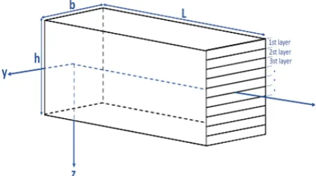
In this research, by using the Timoshenko Beam theory (TBT) and applying the principle of virtual work, the governing equations were extracted. In this theory, the eﬀects of shear deformation and bending moment are considered simultaneously. Considering the nonlinear behavior of the SMA, the amount of MVF varies from point to point, thus the properties of the SMA beam are diﬀerent at each point of the beam. To accomplish the previously stated goal, the SMA beam thickness was divided into an acceptable number of layers, where in each layer, through-the-thickness of the beam, the MVF is assumed constant (Fig. 1).

Fig. 1. Geometry and coordinate system of the SMA beam.

The displacement ﬁeld of the beam in TBT is ob-tained as follows [9]:

u1=u0(x) +zϕx,

u2= 0 (14)

u3=w0(x)

where (u1u2u3) are the displacements of a point along

the (x y z) axes, (u0 w0) are the displacements of a

point on the mid-plane of an undeformed beam, and ϕx is the rotation (about the y-axis) of a transverse

straight line.

With respect to the Von Karman strain relations, the axial and shear components of the strain tensor are expressed in the following equations:

εxx=

∂u1 ∂x + 1 2 ( dw0 dx )2

+du0 dx + 1 2 ( dw0 dx )2

+zdϕx dx

=ε2xx+Zε1xx

εxz=ϕx+

dw0

dx (15)

ε0xx=

du0 dx + 1 2 ( dw0 dx )2

ε1_xx=dϕx dx

By using the principle of virtual displacements, the necessary weak statements of the TBT, can be writ-ten as:

δW ≡δW1+δWE= 0

δW1=

∫ L

0

∫

A

(σxxδεxx+σxzδεxz)dAdx

= ∫ L

0

∫

A

(σxx(δσxx0 +zδε

1

xx) +σxzδεxz)dAdx

= ∫ L 0 ∫ A ( σxx ( dδu0 dx + dw0 dx dδw0

dx +z dδϕx

dx )

(16)

+σxz

( δϕx+

dδw0

dx ) )

dAdx

δWE=−

[∫ L

0

qδw0dx+

∫ L

0

f δu0dx+ 6

∑

i=1

Qiδ∆i

]

where δW1 and δWE are the virtual strain energy

stored in beam and the virtual work done by exter-nal load applied to beam, respectively. Further, σxx,

σxz, q, f, Qi, and δ∆i are the axial stress, the shear

stress, the distributed transverse load, the distributed axial load, the generalized nodal forces and the virtual generalized nodal displacements, respectively.

The axial and shear stress ofk’th layer are deﬁned as below:

σxxk (ξ) =E k

(ξ)(εkxx−α k

(ξ)(T−T0)−εt k

xx(ξ) )

σxxk (ξ) =E k

(ξ)(εkxx(ξ)−α k

(ξ)(T−T0)−εt k

xx(ξ) ) (17)

In Eq. (17), εk_xx(ξ), εk_xz(ξ), ε_xxtk(ξ), εt_xzk(ξ) and αk(ξ) represent the total axial strain, total shear strain, ax-ial transformation strain, shear transformation strain and thermal expansion coeﬃcient ofk’th layer, respec-tively. Also, Young’s modulus and Poisson’s ratio of k’th layer are obtained as follows:

Ek(ξ) =EA+ξ(EM−EA)

vk(ξ) =vA+ξ(vM−vA)

(18)

The axial and shear transformation strain ofk’th layer, are expressed as:

εt_xxk(ξ) =Hmax σ

k xx(ξ)

√ σk

xx(ξ)2+ 3σxzk (ξ)2

ξ

εt_xzk(ξ) =Hmax 3σ

k xz(ξ)

2√σk

xx(ξ)2+ 3σkxz(ξ)2

ξ

(19)

(5)

resultant, moment resultant, and shear force resultant can written as the following forms:

Nxx(ξ) = N K ∑

k=1 ∫ zk+1

zk

bσkxx(ξ)dz

=

N K ∑

k=1 ∫ xk+1

zk

bEk(ξ)(εkxx−ε tk

xx(ξ) )

dz

Mxx(ξ) = N K ∑

k=1 ∫ z_k₊₁

z_k

bσkxx(ξ)zdz

=

N K ∑

k=1 ∫ zk+1

zk

bEk(ξ)(εkxx−ε tk xx(ξ)

) zdz

Qx(ξ) =Ks N K ∑

k=1 ∫ zk+1

zk

bσkxz(ξ)dz

=Ks N K ∑

k=1 ∫ z_k₊₁

z_k

bEk₍_ξ₎

2(1 +vk₍_ξ₎₎ (

εkxz−εt

k

xz(ξ) )

dz

(20)

whereKsis shear correction factor which gives 5/6 and

bis the width of cross-section of the beam.

Additionally, stiﬀness components of beam are ob-tained through:

Axx(ξ) = N K

∑

k=1

∫ zk+1

zk

bEk(ξ)dz

Bxx(ξ) = N K

∑

k=1

∫ zk+1

zk

bEk(ξ)zdz

Dxx(ξ) = N K

∑

k=1

∫ zk+1

zk

bEk(ξ)z2dz

Sxx(ξ) = N K

∑

k=1

∫ zk+1

zk

bEk(ξ) 2(1 +vk_(ξ))dz

(21)

where Axx(ξ), Bxx(ξ), Dxx(ξ), and Sxx(ξ) are

exten-sional, extensional-bending, bending, and shear stiﬀ-nesses of the beam, respectively.

Substituting Eq. (21) in Eq. (20) and using Eq. (15), Eq. (20) is rewritten as below:

Nxx(ξ) = N K ∑ ∫ xk+1

zk

bEk(ξ)

{( du0(ξ)

dx +

1 2

( dw0(ξ)

dx )

+zdϕx(ξ) dx

)

−εtxxk }

dz=Axx(ξ) [

du0(ξ) dx +

1 2

( dw0(ξ)

dx )2]

+Bxx(ξ) (

dϕx(ξ) dx

)

−Ns(ξ)

Mxx(ξ) = N k ∑

k=1 ∫zk+1

zk

bEk(ξ)

{( du0(ξ)

dx

+1 2

( dw0(ξ)

dx )2

+zdϕx(ξ) dx

)

−εtxxk }

zdz (22)

=Bxx(ξ) [

du0(ξ) dx +

1 2

( dw0(ξ)

dx )2]

+Dxx(ξ) (

dϕx(ξ) dx

)

−Ms(ξ)

Qx(ξ) =Ks N K ∑

k=1 ∫ zk+1

zk

bEk(ξ) 2(1 +νk₍_ξ₎₎

{ ϕx(ξ) +

dw0(ξ) dx −ε

tk xz

}

=Sxx(ξ) (

ϕx(ξ) + dw0(ξ)

dx )

−Qs(ξ)

where Ns_(ξ),_Ms_{(ξ) and}_Qs_{(ξ) are the axial force}

re-sultant, moment resultant and shear force rere-sultant, resulting from the axial and shear components of the transformation strain tensor, respectively and can be expressed as:

Ns(ξ) =

N K

∑

k=1

z∑k+1

zk

bEk(ξ)εtxxk(ξ)dz

Ms(ξ) =

N K

∑

k=1

∫ zk+1

zk

bEk(ξ)εtxxk(ξ)zdz (23)

Qs(ξ) =Ks N K

∑

k=1

∫ zk+1

zk

bEk(ξ) 2(1 +νk_(ξ))ε

tk xz(ξ)dz

4. Finite Element Modeling

In this research, for the purpose of investigating SMA beam bending, with respect to the nonlinearity of gov-erning equations, which includes nonlinear material and nonlinear geometry, an iterative nonlinear ﬁnite el-ement model was developed. For the purpose of obtain-ing characteristic of ﬁnite element beam, the Galerkin weighted-residual method was used.

The displacement components of the points on the center plane of the beam are estimated using the La-grange interpolation functions and can be written as follows [9]:

ue₀(ξ) =

m

∑

j=1

uj(ξ)ψ

(1)

j ,

we₀(ξ) =

n

∑

j=1

wj(ξ)ψ

(2)

j , (24)

ϕe_x(ξ) =

p

∑

j=1

sj(ξ)ψ

(3)

(6)

where uj(ξ), wj(ξ) and sj(ξ) are axial displacement,

transverse displacement and rotation of element nodes, respectively. Furthermore, in this study, for all three expressions of Eq. (24), quadratic Lagrange interpo-lation functions (m, n, p= 3) were used which are ob-tained as follows:

ψ1(r) =

1

2r(r−1),

ψ2(r) = 1−r2 (25)

ψ3(r) =

1

2r(r+ 1)

According to Eq. (24) and δu0(ξ) =

∑m j=1ψ

(1)

j , it

can be concluded thatδw0(ξ) =

∑n j=1ψ

(2)

j δwj(ξ) and

δϕx(ξ) =

∑p j=1ψ

(3)

j δsj(ξ) By substitution of Eq. (16),

expressions ofK_ijαβ(ξ) andF_iγ(ξ) (α, β, y= 1,2,3), are expressed as follows:

K_ij11(ξ) = ∫ xb

xa

Ae_xx(ξ)dψ

(1)

i

dx dψ(1)_j

dx dx

K_ij12(ξ) = 1 2

∫ xb

xa

Ae_xx(ξ)dw0(ξ) dx

dψ_i(1) dx

dϕ(2)_j dx dx

Kij13(ξ) =

∫ xb

xa

Bexx(ξ)

dψ_i(1) dx

dψ(3)_j dx dx

K_ij21(ξ) = ∫ xb

xa

Ae_xx(ξ)dw0(ξ) dx

dψ(1)_i dx

dψ_j(2) dx dx

K_ij22(ξ) = ∫ xb

xa

S_xxe (ξ)dψ

(2)

i

dx dψ(2)_j

dx

+1 2

∫ xb

xa

Ae_xx(ξ) (

dw0(ξ)

dx )2

sψ_i(2) dx

dψ(2)_j dx

K_ij23(ξ) = ∫ xb

xa

S_xxe (ξ)dψ

(2) i dx ψ (3) j dx + ∫ xb

xa

Be_xx(ξ)dw0(ξ) dx

dψ(2)_i dx

dψ_j(3) dx dx

K_ij31(ξ) = ∫ xb

xa

Be_xx(ξ)dψ

(3)

i

dx dψ(1)_j

dx dx

Kij32(ξ) =

∫ xb

xa

Sxxe (ξ)ψ

(3)

j

dψ_i(2) dx dx

+1 2

∫ xb

xa

B_xxe (ξ)dw0(ξ) dx

dψ_i(3) dx

dψ_j(2) dx dx

K_ij33(ξ) = ∫ xb

xa (

De_xx(ξ)dψ

(3)

i

dx + dψ_j(3)

dx + (26)

Se_xx(ξ)ψ(3)_j ψ(3)_j )

dx

Fi1(ξ) =

∫ xb

xa {

ψ_i(1)f+Ns(ξ)dψ

(1)

i

dx }

dx

+Qe₁(ξ)ψ(1)_i (xa) +Qe4(ξ)ψ (1)

i (xb)

F_i2(ξ) = ∫ xb

xa {

ψ_i2q+Qs(ξ)dψ

(2)

i

dx +N

s_(ξ)

( dw0(ξ)

dx )

dψ(2)_i dx

}

F_i3(ξ) = ∫ xb

xa {

Qs(ξ)ψ_i(3)+Ms(ξ)dψ

(3)

i

dx }

dx

+Qe3(ξ)ϕ (3)

i (xa) +Qe6(ξ)ψ (3)

i (xb)

where generalized nodal forces are given by:

Q1(ξ) =−Nxx(ξ)(0)

Q4(ξ) =Nxx(ξ)(L)

Q2(ξ) =−

[

ϕx(ξ) +Nxx(ξ)

∂w0(ξ)

∂x ]

x=0

,

Q5(ξ) =

[

ϕx(ξ) +Nxx(ξ)

∂w0(ξ)

∂x ]

x=L

Q3(ξ) =−Mxx(ξ)(0),

Q6(ξ) =Mxx(ξ)(L)

(27)

5. Numerical Results and Discussion

In this section, the numerical results of bending of SMA beam under diﬀerent loading and unloading conditions and diﬀerent support conditions are presented in con-stant temperature conditions (T =T0= 300K). To

val-idate the applied formulation of the present study, the problems of three-point bending and cantilever beam bending were modeled and the outcomes were com-pared with the experimental and numerical results pre-sented by Mirzaeifar et al. [7].

The properties of the Ni-Ti alloy used in the present work are presented in Table 1 [10].

(7)

transverse loadq0 = 12

KN

m , was loaded and unloaded in the number of different elements. The convergence criterion was chosen for difference of deflections, less than 1.6×10−5m. Finally, the total of 16 second-order elements were selected.

Table 1

Material parameters of Ni-Ti SMA used in the present work. Material parameter Value (unit)

H 0.05

As 272.7K

Af 281.6K

Ms 254.9K

Mf 238.8K

vA₌_vM _0.42

EA _72GPa

EM _30GPa

ρcA₌_ρcM _2.6_×₁₀6_J/(m3_K)

(dσ/dT)A _8.4_×₁₀6_J/(m3_K)

ρ∆s0=−H(dσ/dT)A −0.42×106J/(m3K)

∆c 0

5.1. Validation

In order to validate the proposed formulation, the re-sults of the simulation of the three-point bending test and the bending of cantilever beam were compared with the results presented by Mirzaeifar et al. [7].

5.1.1. Three-point Bending Test

In this test, loading and unloading of the hinged-hinged SMA beam, with the length of 170mm and the rect-angular cross-section with the height of 3mm and the width of 7.5mm, subjected to the transverse load ap-plied in the middle of the beam was investigated. In or-der to provide constant temperature conditions, load-ing and unloadload-ing were done incrementally.

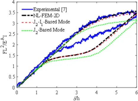
Fig. 2 shows the non-dimensional load-deflection results of the beam using the two-dimensional nonlin-ear finite element model (NL-FEM-2D) presented in this study and the experimental and numerical results presented by Mirzaeifar et al. [7]. As it is shown in this figure, at the loading phase the outcomes of the NL-FEM-2D model are very close to the experimental results. However, there is some differences between the results at the unloading phase. This difference results from the fact that the proposed constitutive equations cannot properly predict the stress-strain conditions at the unloading phase and the difference becomes even greater when the material starts the unloading phase before it fully reaches the martensitic phase. In con-trast, by increasing the cross-section thickness and modifying the transformation hardening function, the observed difference in the unloading phase can be re-duced. The results show that the NL-FEM-2D model can predicts material behavior better than J2 model

does, in both loading and unloading phases. The pre-sented model is closer to the experimental results than theJ2−J1 model.

Fig. 2. Non-dimensional load-deﬂection results ob-tained from three-point bending test and theoretical solutions.

In this section, the SMA beam with the length of 100mm and the rectangular cross-section with the height of 10mm and the width of 1.5mm, which was subjected to the transverse load at the free end of the beam, is simulated. In order to provide constant tem-perature conditions, loading and unloading were done incrementally. To this end, the ﬁnal load ofF = 210N was applied to the beam at 42 steps, with each step adding the value of 5N to the amount of loading. Sim-ilarly, for the unloading phase, at each step, the value 5N was substracted from the amount of unloading.

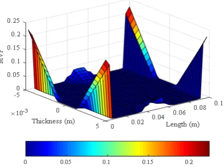
Fig. 3 and Fig. 4 respectively indicate the results of the distribution of normal stress and the MVF at the clamped edge in correspondence with the end of the loading, along with the numerical results presented by Mirzaeifar et al. [7]. As can be seen in Fig. 3, the max-imum value of normal stress occurred in the upper and lower edges of the cross-section. While the level of nor-mal stress in the core of the beam is negligible. Based on what has been said, Fig. 4 can be interpreted in this way that maximum stress occurs in the upper and lower edges of the cross-section, where consequently the most phase transformation is seen. On the other hand, by moving toward the core of the beam, with decrease in the stress level, the phase transformation is reduced such that the MVF in the core of the beam is zero. The results show that the outcomes of the formulation presented in this study with other numerical analyses are in good agreement.

5.2. Other Results

(8)

men-tioned in Section 5.2.1.

Fig. 3. Normal stress distribution through-the-thickness of the cantilever SMA beam at the clamped edge (corresponding to the end of the loading phase).

Fig. 4. MVF distribution through-the-thickness of the cantilever SMA beam at the clamped edge (corre-sponding to the end of the loading phase).

5.2.1. An Investigation of Different Support Conditions of SMA Beam

In this section, the mentioned SMA beam was

sub-jected to the distributed transverse load q0 = 23

KN m at different support conditions. In order to provide quasi-static conditions, the final load was subjected to the beam as a series of small loads. Figs. 5 to 10 show the distribution of the MVF along the length and through-the-thickness of the SMA beam for differ-ent support conditions, which the results correspond to the end of loading phase.

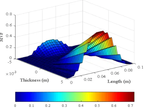
Fig. 5 shows that the maximum phase transfor-mation occurs in the in the upper and lower edges of the clamped cross-sections of the beam, also the mid-section of the beam length, but is much less than the phase transformation at the clamped cross-sections. In addition, due to the nonlinearity of the strain ﬁeld, in the near sections of two ends of the beam, the phase

transformation at the upper edge of the beam which is under tensile stress is greater than the lower edge of the beam which is under compression stress. In other words, the distribution of stress in the beam is not symmetric. This state also occurs at the mid-section of the beam with the diﬀerence that this time the lower edge, which is under tensile stress, shows a greater phase transformation. By moving toward the core of the beam, the phase transformation decreases, with de-crease in stresses, so that the layers around the core of the beam completely remain in the austenite phase.

Fig. 5. Distribution of MVF for all points along the length and the through-the-thickness of the clamped-clamped SMA beam (corresponding to the end of the loading phase).

In Fig. 6, the support conditions are similar to Fig. 5 except that the nonlinear component of the strain ﬁeld is neglected in the modeling of the beam. It causes a symmetric distribution of stress and, as a result, the symmetric distribution of the MVF in the cross-sections of the middle and two ends of the beam.

(9)

In this part one of the clamped supports was re-placed with a pinned support, and as can be seen in Fig. 7, it increased the asymmetric distribution of MVF through-the-thickness of the beam. Increasing the deﬂection of the beam, increases the phase trans-formation in the layers of cross-sections of clamped end and middle of the beam.

Fig. 7. Distribution of MVF for all points along the length and the through-the-thickness of the clamped-pinned SMA beam (corresponding to the end of the loading phase).

For more study, one of the clamped supports of Fig. 5 was replaced with a hinged support. As can be seen in Fig. 8 by removal of in-plane forces in one of the supports, although increasing the deflection increases the stress and MVF at the middle and clamped cross-sections of beam, it leads to the loss of the effect of the nonlinear strain field components and reveals the symmetric distribution of MVF through-the-thickness of the beam.

Fig. 8. Distribution of MVF for all points along the length and the through-the-thickness of the clamped-hinged SMA beam (corresponding to the end of the loading phase).

As can be seen in Fig. 9, in the case of pined-pined

supporting, the phase transformation occurs only at the middle of the beam although the eﬀect of the non-linear strain ﬁeld is as well apparent in the asymmetric distribution of the MVF.

Fig. 9. Distribution of MVF for all points along the length and the through-the-thickness of the pinned-pinned SMA beam (corresponding to the end of the loading phase).

Finally, for pinned-hinged and hinged-hinged sup-port conditions the same results were obtained as shown in Fig. 10.

Fig. 10. Distribution of MVF for all points along the length and the through-the-thickness of the hinged-hinged SMA beam (corresponding to the end of the loading phase).

(10)

Fig. 11. Non-dimensional deﬂection of neutral axis of SMA beam for diﬀerent support conditions (corre-sponding to the end of the loading phase).

5.2.2. Different Force Conditions of SMA Beam

In this section, further results are presented for the loading of cantilever beam which was mentioned in section 5.1.2. To this end, the behavior of the SMA beam at ﬁve forces of 210N, 175N, 125N, 75N, and 25N in both loading and unloading phases were inves-tigated separately. Figs. 12 to 17 show the distribu-tion of stress through-the-thickness of the beam at the clamped cross-section of beam for diﬀerent force con-ditions during loading and unloading phases.

The distribution of normal stress through-the-thickness of the beam in the loading steps is shown in Fig. 12. As can be seen for the forces of 75N and 25N, where there is no phase transformation in the SMA beam, the distribution of stress is linear through-the-thickness of the beam. With the increase in force and the onset of the phase transformation in the SMA beam, the nonlinear distribution of stress intensiﬁes. With increasing force, variation of stress increases at the upper and lower edges as well.

Fig. 13, similar to Fig. 12, shows the distribution of normal stress through-the-thickness of the beam, with the diﬀerence that the unloading phase is considered this time. As can be seen in the three forces of 210N, 175N, and 125N, the SMA beam is being elastically unloaded and no phase transformation occurs in the material, therefore the distribution of stress in the lay-ers is the same and only the stress level is reduced. Another important point is to compare the SMA beam behavior in the 75N force in loading and unloading phases, which shows that during the loading the phase transformation has not yet occurred, but during the unloading phase, the phase transformation is seen in this force. In both loading and unloading phases, the stress decreases by moving toward the core of the beam through-the-thickness of the beam as well.

Fig. 12. Normal stress distribution through-the-thickness of the cantilever SMA beam at the clamped edge for diﬀerent force conditions (corresponding to the loading phase).

Fig. 13. Normal stress distribution through-the-thickness of the cantilever SMA beam at the clamped edge for diﬀerent force conditions (corresponding to the unloading phase).

Fig. 14 and Fig. 15 show the distribution of shear stress through-the-thickness of the beam in loading and unloading steps, respectively. In elastic conditions, the shear stress in the SMA beam is constant. When the phase transformation occurs, the shear stress distribu-tion becomes nonlinear. By moving toward the core of the beam through-the-thickness of the beam, the shear stress increases. It intensiﬁes with increasing phase transformation in material.

(11)

close to zero. In contrast, by increasing the force, the intensity of the shear stress increases and causes the Von Mises stress, in the middle layer of the , to be-come non-zero. Moreover, the fractures seen in the stress distribution diagrams indicate the occurrence of a phase transformation in SMA beam.

Fig. 14. Shear stress distribution through-the-thickness of the cantilever SMA beam at the clamped edge for diﬀerent force conditions (corresponding to the loading phase).

Fig. 15. Von Mises stress distribution through-the-thickness of the cantilever SMA beam at the clamped edge for diﬀerent force conditions (corresponding to the loading phase).

6. Summary and Conclusions

In this research, the nonlinear superelastic bending of SMA beam with consideration of the material and ge-ometric nonlinearity eﬀects, which were coupled to-gether, was investigated. For modeling of SMA, the Boyd-Lagoudas 3D model, which were properly re-duced to two dimensions, were used. Due to the non-linearity of the SMA, the iterative nonlinear ﬁnite

el-ement model of two dimensional (NL-FEM-2D model) was presented for SMA beam modeling. The study of the simultaneous eﬀects of large strains and property changes in the whole beam on the superelastic bending of SMA beam, is one of the most important results of this research as well. The most important results are as follows:

Fig. 16. Shear stress distribution through-the-thickness of the cantilever SMA beam at the clamped edge for diﬀerent force conditions (corresponding to the unloading phase).

Fig. 17. Von Mises stress distribution through-the-thickness of the cantilever SMA beam at the clamped edge for diﬀerent force conditions (corresponding to the loading phase).

• By applying the external force suﬃciently large to the beam, a phase transformation in the mate-rial and, accordingly, non-zero MVF are resulted.

• As the load increases, the MVF and consequently, the level of hysteresis increases, which decreases the modulus of elasticity and strength of the ma-terial and increases the deﬂection of SMA beam.

(12)

stress-related, it can be said that the properties of SMA beam are variable in diﬀerent points of the SMA beam, and as a result, the material exhibits non-homogeneous behavior when sub-jected to bending load.

• The numerical method presented in this research can be a suitable alternative for expensive exper-imental experiments and complex calculations.

As far as only superelastic behavior of the SMA beam was investigated in this study, by considering the ther-mal eﬀects of the equations and analyzing the thermo-mechanical eﬀects of the SMA beam, it is possible to obtain more complete results.

References

[1] K. Otsuka, C.M. Wayman, Shape Memory Materi-als. Cambridge University Press, Cambridge,(1998).

[2] D.C. Lagoudas, Shape Memory Alloys Modeling and Engineering Applications,Springer,(2007).

[3] M.B. Jaber, H. Smaoui, P. Terriault, Finite element analysis of a shape memory alloy three-dimensional beam based on a ﬁnite strain description., Smart. Mater. Struct., 17 (2008) 045005:1-11.

[4] T. Mineta, T. Mitsui, Y. Watanabe, S. Kobayashi, Y. Haga, M. Esashi, An active guide wire with

shape memory alloy bending actuator fabricated by room temperature process., Sens. Actuators., 97 (2002) 632-637.

[5] Y. Gillet, E. Patoor, M. Berveiller. Structure cal-culations applied to shape memory alloys. Journal De Physique IV., 5 (1995) 343-348.

[6] M. Baghani, H. Mohammadi, R. Naghdababi, An analytical solution for shape-memory polymer Eu-lerBernoulli beams under bending, Int. J. Mech. Sci., 84 (2014) 84-90.

[7] R. Mirzaeifar, R. Desroches, A. Yavari, K. Gall, On superelastic bending of shape memory alloy beams, Int. J. Solids. Struct., 50 (2013) 1664-1680.

[8] M. Botshekanan Dehkordi, S.M.R. Khalili, E. Car-rera, M. Sharyat, Non-linear dynamic analysis of a sandwich beam with pseudoelastic SMA hybrid composite faces based on higher order ﬁnite ele-ment theory, Compos. Struct., 96 (2013) 243-255.

[9] J.N. Reddy, An Introduction to Nonlinear Finite Element Analysis, Oxford University Press,Oxford, (2005).