https://doi.org/10.5194/gmd-10-2365-2017 © Author(s) 2017. This work is distributed under the Creative Commons Attribution 3.0 License.
STRAPS v1.0: evaluating a methodology for predicting electron
impact ionisation mass spectra for the aerosol mass spectrometer
David O. Topping1,2, James Allan1,2, M. Rami Alfarra1,2, and Bernard Aumont3
1School of Earth and Environmental Science, University of Manchester, Manchester, M13 9PL, UK 2National Centre for Atmospheric Science, University of Manchester, Manchester, M13 9PL, UK 3LISA, UMR CNRS 7583, Universite Paris Est Creteil et Universite Paris Diderot, Creteil, France
Correspondence to:David O. Topping ([email protected]) Received: 20 December 2016 – Discussion started: 17 January 2017 Revised: 11 April 2017 – Accepted: 5 May 2017 – Published: 27 June 2017
Abstract. Our ability to model the chemical and thermo-dynamic processes that lead to secondary organic aerosol (SOA) formation is thought to be hampered by the com-plexity of the system. While there are fundamental models now available that can simulate the tens of thousands of re-actions thought to take place, validation against experiments is highly challenging. Techniques capable of identifying indi-vidual molecules such as chromatography are generally only capable of quantifying a subset of the material present, mak-ing it unsuitable for a carbon budget analysis. Integrative analytical methods such as the Aerosol Mass Spectrometer (AMS) are capable of quantifying all mass, but because of their inability to isolate individual molecules, comparisons have been limited to simple data products such as total or-ganic mass and the O : C ratio. More detailed comparisons could be made if more of the mass spectral information could be used, but because a discrete inversion of AMS data is not possible, this activity requires a system of predicting mass spectra based on molecular composition.
In this proof-of-concept study, the ability to train super-vised methods to predict electron impact ionisation (EI) mass spectra for the AMS is evaluated. Supervised Training Re-gression for the Arbitrary Prediction of Spectra (STRAPS) is not built from first principles. A methodology is constructed whereby the presence of specific mass-to-charge ratio (m/z) channels is fitted as a function of molecular structure before the relative peak height for each channel is similarly fitted using a range of regression methods. The widely used AMS mass spectral database is used as a basis for this, using unit mass resolution spectra of laboratory standards.
Key to the fitting process is choice of structural informa-tion, or molecular fingerprint. Our approach relies on using supervised methods to automatically optimise the relation-ship between spectral characteristics and these molecular fin-gerprints. Therefore, any internal mechanisms or instrument features impacting on fragmentation are implicitly accounted for in the fitted model. Whilst one might expect a collection of keys specifically designed according to EI fragmentation principles to offer a robust basis, the suitability of a range of commonly available fingerprints is evaluated.
Given the limited number of compounds used within the AMS training dataset, it is difficult to prescribe which com-bination of approach would lead to a robust generic model across all expected compositions. Nonetheless, the study demonstrates the use of a methodology that would be im-proved with more training data, fingerprints designed ex-plicitly for fragmentation mechanisms occurring within the AMS, and data from additional mixed systems for further validation. To facilitate further development of the method, including application to other instruments, the model code for re-training is provided via a public Github and Zenodo software repository.
1 Introduction
Volatile organic compounds (VOCs), emitted from both nat-ural and anthropogenic sources, are oxidised in the atmo-sphere to form lower-volatility species that condense onto aerosol particles or contribute to new particle formation (Laaksonen et al., 2008; Sipila et al., 2016; Ehn et al., 2014). With an enormous number of species that are present, this diversity in chemistry is reflected in the extensive range of species and chemical signatures identified in ambient stud-ies (Hamilton et al., 2013). Within atmospheric science, it is desirable to develop models for secondary organic aerosol (SOA) formation based on a given set of precursors and photochemical processing. Within most global and regional models, often-used techniques include modelling representa-tive photochemical yields from specific precursors and tun-ing accordtun-ingly (Spracklen et al., 2011) or employtun-ing a para-metric model such as the volatility basis set (Robinson et al., 2007). While both of these approaches can deliver re-alistic absolute concentrations, because they are not based on explicit physical processes, their predictive skill is al-ways subject to question (Hallquist et al., 2009; Bergström et al., 2012). It is therefore desirable to develop SOA models based around actual molecular processes and kinetics con-strained through laboratory experiments (where available), such that this skill can be evaluated. Such models rely on explicit chemical mechanisms such as the Master Chemical Mechanism (MCM) (Saunders et al., 1997) or the GECKO model (Aumont et al., 2005). While this mechanistic ap-proach has resulted in poor performance in terms of abso-lute mass concentrations in the past (Volkamer et al., 2006), much of this shortfall can be accounted for by not con-sidering all precursors (in particular the semi-volatile and intermediate-volatility organic matter), unexpected processes likely to produce lower-volatility products, e.g. oligomerisa-tion and autoxidaoligomerisa-tion (Ehn et al., 2014), and inadequacies associated with phase partitioning models (Barley and Mc-Figgans, 2010; Valorso et al., 2011; McVay et al., 2016). As the availability of data regarding these has improved and thus our understanding of these processes matured, the
per-formance of the models has become more realistic (Mc-Vay et al., 2016). The development of more applicable ex-plicit models has been facilitated by the ability to automat-ically predict processes rather than prescribe them (Aumont et al., 2012, 2005), as has been implemented in the Gener-ator of Explicit Chemistry and Kinetics of Organics in the Atmosphere (GECKO-A) and the forthcoming version 4 of the MCM (http://gotw.nerc.ac.uk/list_full.asp?pcode=NE% 2FM013448%2F1). This can be supplemented by the au-tomated prediction of properties important for partitioning, using generalised informatics tools such as UManSysProp (Topping et al., 2016). While it is unlikely that such complex models would be used directly for large-scale Eulerian chem-ical transport and climate models, and uncertainties with re-gards to fundamental properties remain (Bilde et al., 2015), they are still highly useful for benchmarking and providing the parameters for simpler models.
Comparison of model output with measurements in the ambient air and in the laboratory is required to test model accuracy. With current analytical methods, it is impossi-ble to detect and quantify every compound in the particle even if we can predict compound-by-compound speciation. While there are techniques capable of resolving a large num-ber of molecules, such as electrospray ionisation and two-dimensional gas chromatography (Noziere et al., 2015), com-prehensively calibrating for and thus providing quantitative data on the abundances of the molecules is difficult. The AMS, which is often used in chamber and flow tube experi-ments, is capable of delivering data on the total mass concen-tration of organic matter and some other simple top–down metrics such as the O : C ratio (Aiken et al., 2007). However, this does not provide the ideal constraint of such models.
While the mass spectral data can be further investigated through inspection of markers at specificm/zchannels (such as 43 and 44) (Ng et al., 2011), such data tend to be qual-itative and result in speculative conclusions (Morgan et al., 2010). In theory, the data across the mass spectrum could be more systematically compared with the modelled data if knowledge of the instrument response to molecular features could be invoked in a general fashion (Ehn et al., 2014).
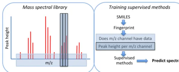
In this proof-of-concept study we evaluate a methodol-ogy to bridge existing model–measurement comparison. A database of the AMS mass spectral responses to various molecules has been built up over the years, and this has been used to characterise the response of certain key peaks to cer-tain functional groups (Ulbrich et al., 2009; Ehn et al., 2014). In this study we use that information to develop and evaluate regression software that predicts an AMS spectrum based on the predicted aerosol composition (Fig. 1).
Figure 1.Schematic of the workflow used in the training process. For a normalised mass spectrum, the SMILEs string associated with each compound is combined with a given molecular fingerprint to train methods to predict the occurrence of a givenm/zchannel and then a peak height.
spectrometry for small to medium sized molecules from first principles. Whilst that study documents improving general applicability, they are not immediately suitable for predicting AMS mass spectra because the thermal desorption promotes further fragmentation and, in some cases, pyrolysis (Cana-garatna et al., 2015). While the standard AMS analysis takes these processes into account through empirical calibrations, the exact physical processes taking place within the vaporiser system are still the subject of considerable debate (Murphy, 2016; Drewnick et al., 2015; Robinson et al., 2016), so the bottom–up modelling of this is not possible with the current state of knowledge.
Distinct from all previous approaches, the approach pre-sented here relies on supervised learning methods to auto-matically optimise the relationship between spectral charac-teristics and molecular features from the instrument in ques-tion. Therefore, any internal mechanisms or instrument fea-tures impacting on fragmentation are implicitly accounted for in the fitted model.
In Sect. 2 the methodology behind constructing a predic-tive model is presented, whereas Sect. 3 focuses on results regarding the accuracy of a model with respect to compar-isons with spectra for individual components. In addition, we present results from simulating the mass spectra ofα-pinene aerosol using the GECKO-A model before we discuss future data requirements in Sect. 4.
2 Methodology
Figure 1 displays the workflow used in building the predic-tive model. First, a model is trained to predict the occurrence of specificm/zchannels as a function of molecular compo-sition before a model for eachm/zchannel is trained to pre-dict peak height within that channel. It is worthwhile detail-ing the molecular information used to train each model. Each molecule has varying levels of structural features, which can be written in terms of a “fingerprint”. This fingerprint is a nu-merical identification of a given structure that can equally be thought of as stoichiometric information for distinct features.
For example, for a collection of 10 compounds, we would construct a matrix of stoichiometric information where each row represents a specific molecule and each column the sto-ichiometry of a given feature. We now refer to each column as a “key”, which might be a specific functional group or fea-ture associated with that molecule. We retain the use of the word “key” since it can provide more generic information than a functional group. To re-iterate, we refer to the entire row as the molecular fingerprint. For example, identifying the occurrence of carboxylic acid groups is a key within the AIOMFAC fingerprint (Zuend et al., 2011). We then take this information and use it to train a model to predict both the oc-currence of a specificm/zchannel and then peak heights.
To re-iterate, in constructing a model that can predict AMS mass spectra, a library of compounds with measured spec-tra are used to spec-train a series of regression techniques. This collection of molecules, represented as SMILES strings, is parsed to produce a matrix where each column represents the stoichiometry of a particular key, or feature. This entire matrix is used to fit a predict model for eachm/zchannel.
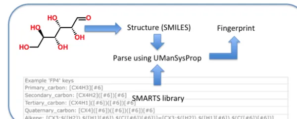
Figure 2.Basic schematic of interrogating a SMILES string with a SMARTS library to construct a molecular fingerprint.
a broad range of applications. The MACCS fingerprint pro-vides up to 162 unique keys of any given molecule, the FP4 fingerprint featuring up to 320. The current implementation of the MACCS keys from the Pybel package (O’Boyle et al., 2011) is used, whereas the FP4 keys are extracted from the RDKit open-source informatics package (http://www.rdkit. org/docs/index.html). Each key is represented in the UMan-SysProp package (Topping et al., 2016) using SMARTS no-tation, and each molecule using the SMILES format. The matrix of keys used to fit each method is constructed by sys-tematically parsing each molecule. Figure 2 demonstrates the use of the MACCS SMARTS to populate a matrix of keys. There are some common features between each fingerprint library, but also a range of differences. For example, all li-braries identify the presence of the CH2 group, but then dif-fer in the optional connecting groups. The FP4 keys cycle through systematic groupings, such as primary carbon, sec-ondary carbon, tertiary carbon, primary alcohol, secsec-ondary alcohol, and tertiary alcohol. Similar groups are detected us-ing the activity coefficient and vapour pressure keys. The full collection of SMARTS keys can be found in the source code and we discuss suggestions for future work on refining fin-gerprints in Sect. 4. Please refer to the code availability sec-tion.
With regards to the supervised methods used, an ensemble tree is trained to predict the occurrence of specificm/z chan-nels as a function of any given fingerprint. To predict peak height perm/zchannel, we evaluate a number of supervised methods available in the SciKit-learn package: generalised linear methods, support vector machines (with three sepa-rate kernels), stochastic gradient descent, Bayesian ridge, or-dinary least squares, decision trees, and ensemble methods (Pedregosa et al., 2011). There are a number of other meth-ods available; however, as we will discuss in Sect. 4, the results from this study demonstrate a potential, whilst fur-ther data are needed to confirm general applicability, includ-ing the use of other methods. For a brief overview of each method, we refer the reader to Ruske et al. (2017), and ref-erences therein. Before training each method, the matrix of identified keys was standardized between zero and one using
the MinMaxScaler pre-processing feature within the Scikit learn package. In addition, the use of variable selection is de-signed to use only those features deemed important to con-struct fingerprint–peak height relationships to try and miti-gate any underfitting or overfitting. The sensitivity to these procedures is discussed in Sect. 3.2. To compare modelled and measured mass spectra, the cosine angle from a dot prod-uct of the two is used, focusing on specificm/zchannels that are typically found as features within atmospheric and smog chamber mass spectra (Ulbrich et al., 2009): 15, 18, 28, 29, 39, 41, 43, 44, 50, 51, 53, 55, 57, 60, 73, 77, 91.
The ability of each method to replicate the entire database is first evaluated. Whilst training on a subset and comparing with the entire database will test wider applicability, this ini-tial comparison quantifies the appropriateness of the different fingerprints in building an accurate model.
3 Results
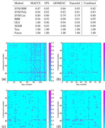
effi-Table 1.Median cosine angle between measured and predicted spectra when fitting to the entire dataset as a function of molecular fingerprint (given above each column). Please note that the term “Combined” refers to a combination of all individual fingerprints into one. The method labels are as follows: SMV (support vector machine with three kernels (RBF, Poly(nomial) and Lin(near))); BRR: Bayesian ridge; OLS: ordinary least squares; SGDR: stochastic gradient descent; Tree: decision tree; and Forest: random forest.
Method MACCS FP4 AIOMFAC Nanoolal Combined
SVM RBF 0.87 0.85 0.86 0.85 0.85
SVM Poly 0.84 0.83 0.82 0.81 0.83
SVM Lin 0.80 0.80 0.79 0.79 0.80
BRR 0.94 0.92 0.90 0.91 0.95
OLS 1.00 0.96 0.94 0.94 0.99
SGDR 0.88 0.82 0.80 0.80 0.89
Tree 1.00 1.00 1.00 1.00 1.00
Forest 1.00 1.00 1.00 1.00 1.00
Figure 3.Sparsity of keys extracted (xaxes) from each compound (yaxes) as a function of the molecular fingerprint used (a: MACCS;b: FP4;c: AIOMFAC;d: Nanoolal). Keys are coloured according to normalised stoichiometry across all compounds.
cacy of using pre-defined fingerprints as they are available in the literature or within existing open-source software pack-ages. The exact physical processes taking place within the instrument are still the subject of considerable debate.
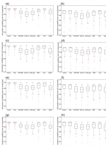
Table 1 presents the median cosine angle of modelled spectra fitted to the entire AMS database derived from the different supervised methods and different fingerprints, ei-ther isolated or combined into one, to two decimal places. The left-hand-side box-plots in Fig. 4a–d display the entire cosine angle spread for each method for the isolated MACCS
Figure 4. (a)Spread of the cosine angle between experimental and predicted mass spectra (yaxes) for all 100 compounds in the AMS library as a function of the supervised method (xaxes) using the MACCS fingerprint. Left: using all compounds in the training process. Right: using 80 % of the compounds in the training process with variable selection. The method labels are as follows: SMV (support vector machine with three kernels (RBF, Poly(nomial), and Lin(near))); BRR: Bayesian ridge; OLS: ordinary least squares; SGDR: stochastic gradient descent; Tree: decision tree; and Forest: random forest.(b)Spread of the cosine angle between experimental and predicted mass spectra (yaxes) for all 100 compounds in the AMS library as a function of the supervised method (xaxes) using the FP4 fingerprint. Left: using all compounds in the training process. Right: using 80 % of the compounds in the training process with variable selection. The method labels are as follows: SMV (support vector machine with three kernels (RBF, Poly(nomial), and Lin(near))); BRR: Bayesian ridge; OLS: ordinary least squares; SGDR: stochastic gradient descent; Tree: decision tree; and Forest: random forest. (c)Spread of the cosine angle between experimental and predicted mass spectra (yaxes) for all 100 compounds in the AMS library as a function of the supervised method (xaxes) using the AIOMFAC fingerprint. Left: using all compounds in the training process. Right: using 80 % of the compounds in the training process with variable selection. The method labels are as follows: SMV (support vector machine with three kernels (RBF, Poly(nomial), and Lin(near))); BRR: Bayesian ridge; OLS: ordinary least squares; SGDR: stochastic gradient descent; Tree: decision tree; and Forest: random forest.
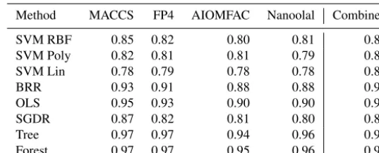
Table 2.Median cosine angle between measured and predicted spectra, using 80% of the compounds in the training process, with variable selection, as a function of molecular fingerprint (given above each column). Please note that the term “Combined” refers to a combination of all individual fingerprints into one. The method labels are as follows: SMV (support vector machine with three kernels (RBF, Poly(nomial) and Lin(near))); BRR: Bayesian ridge; OLS: ordinary least squares; SGDR: stochastic gradient descent; Tree: decision tree; and Forest: random forest.
Method MACCS FP4 AIOMFAC Nanoolal Combined
SVM RBF 0.85 0.82 0.80 0.81 0.85
SVM Poly 0.82 0.81 0.81 0.79 0.82
SVM Lin 0.78 0.79 0.78 0.78 0.80
BRR 0.93 0.91 0.88 0.88 0.94
OLS 0.95 0.93 0.90 0.90 0.98
SGDR 0.87 0.82 0.81 0.80 0.88
Tree 0.97 0.97 0.94 0.96 0.98
Forest 0.97 0.97 0.95 0.96 0.98
in the proceeding analyses. Whichever fingerprint is used, the ranking of performance between supervised methods re-mains similar, with the tree-based methods, ordinary least squares, and Bayesian ridge outperforming stochastic gradi-ent descgradi-ent and all support vector machine kernels. Along with higher median values, the spread of cosine angles from the tree-based methods and ordinary least squares is much lower than all other methods. Whilst the use of MACCS and FP4 provides, in theory, more information, there is some similarity in structural information provided in all keys, as already discussed. For example, each fingerprint identifies key functional groups such as alkanes, alcohol, and ketones, whilst the FP4 and MACCS keys in particular include more positional detail, including relative positions of groups. At least for the 100 compounds in the AMS library, that ad-ditional information leads to a slight increase in cosine an-gle agreement of around 0.02 between methods, if we use only results from Table 1 and Fig. 4. A key objective of this study, noted above, is to demonstrate the use of pre-defined fingerprints in constructing a predictive model. However, it is useful to also demonstrate the efficacy of combining the information from each fingerprint into one, without relating variable performance according to physical processes taking place within the instrument. The performance of combining all fingerprints into one, represented in Table 1 under the col-umn heading “Combined”, illustrates a similar trend in per-formance between methods.
We discuss the significance of values displayed in Table 1 after performance is re-evaluated following a more general approach of training to a subset of compounds, and the use of variable selection, in the next section.
3.2 Training to a subset, variable selection, and dimensionality reduction
Table 2 presents the median cosine angle between modelled and predicted mass spectra, as a function of fingerprint, ei-ther isolated or combined into one, and regression technique,
when training to a subset of the entire database and use of variable selection. To minimise overfitting any model to spe-cific features, the process of variable selection allows us to refit the model to those keys deemed most important. The combination of both strategies might be considered the most suitable test of the methodology presented, with the full spread of statistics presented in the right-hand column of Fig. 4a–d. It should be noted that randomly selecting the sub-set used for training leads to a significant decrease in model performance. This is due to missing keys within the train-ing subset that are deemed important in predicttrain-ing spectra for those compounds outside of the subset. A different ap-proach is to select the subset by maximising the number of keys across each molecule in the training subset, and is used in our proceeding analysis.
Table 3. Median cosine angle between measured and predicted spectra, applying PCA analysis to the “combined” fingerprints, as a function of the number of principal components used given above each column. The method labels are as follows: SMV (support vec-tor machine with three kernels (RBF, Poly(nomial) and Lin(near))); BRR: Bayesian ridge; OLS: ordinary least squares; SGDR: stochas-tic gradient descent; Tree: decision tree; and Forest: random forest.
Method 20 10 8 4
SVM RBF 0.84 0.84 0.85 0.67 SVM Poly 0.83 0.83 0.81 0.79 SVM Lin 0.80 0.80 0.80 0.80
BRR 0.93 0.90 0.89 0.87
OLS 0.94 0.89 0.89 0.87
SGDR 0.89 0.89 0.89 0.88
Tree 0.98 0.98 0.98 0.98
Forest 0.99 0.99 0.99 0.99
demonstrate clear sensitivity to the number of components when combined with the RBF support vector machine ker-nel, performance varying from 0.84 to 0.67 on reducing the number of components from 20 to 4.
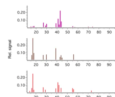
On the significance of the value of the cosine angle, Figs. 5 and 6 display predicted spectra for compounds not included in a training set, along with the cosine angle between mod-elled and measured spectra. From this point on we use iso-lated fingerprints to demonstrate the efficacy of our approach. For oxalic acid, in Fig. 5, the difference in performance be-tween the FP4 and MACCS fingerprint (cosine of 0.83 and 0.77) is apparent through certain features, including the rela-tive proportion of peak heights for the three dominant chan-nels, and the ratio off44tof43. In Fig. 6, a similar pattern is found for leucine, including a marked difference in whether the model predicted non-zero entries acrossf41–f44. Whilst a small subset, these results suggest use of the cosine angle alone is not sufficient to validate model performance, which is confirmed in Sect. 3.3 when applied to theα-pinene sys-tem. Based on these comparisons, a tentative suggestion of using a cosine angle of 0.8 might go some way to clari-fying the performance statistics provided in Tables 1 and 2 and Fig. 4. Indeed, results demonstrate that, whilst statistics in Table 2 and Fig. 4 suggest similar performance for both MACCS and FP4 keys, this performance is composition de-pendent. This reflects sensitivity to information used in the training process and how similarity between performances should be taken with caution in prescribing which method to take forward. This is better highlighted in the proceeding section with regards to a model SOA system.
Results at least suggest the tree-based methods are at least the most stable given the higher range of cosine angles pre-sented in Fig. 4a–d and the decision tree method will be used in all proceeding analysis.
Figure 5.Measured mass spectra for oxalic acid (a)versus pre-dicted mass spectra from an ensemble tree using the FP4 fingerprint (b, cosine of 0.83) and the MACCS fingerprint (c, cosine of 0.77).
Figure 6.Measured mass spectra for leucine(a)versus predicted mass spectra from an ensemble tree using the FP4 fingerprint (b, cosine of 0.70) and the MACCS fingerprint (c, cosine of 0.94).
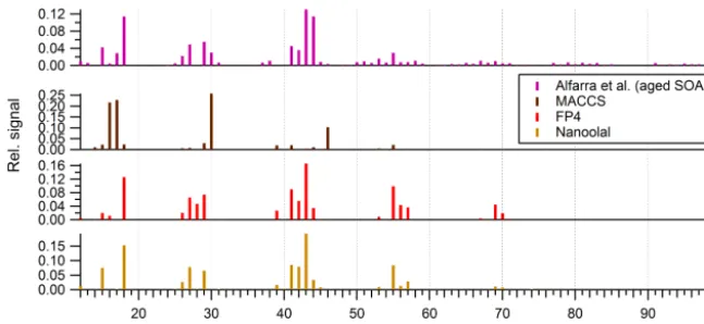
Figure 7.Comparison of the predicted mass spectra ofα-pinene SOA based on the GECKO-A simulation presented by Valorso et al. (2011) using various fingerprinting techniques. These are compared with an actualα-pinene SOA mass spectrum obtained by Alfarra et al. (2013) during a chamber experiment.
be confirmed until more explicit mechanisms are established for α-pinene autoxidation (McVay et al., 2016). One might imagine an ideal sensitivity study would be to use speciated output from these updated models and add additional con-straint to prescribing model performance through a compari-son between measured and predicted mass spectra. Indeed, that is a rationale behind the study presented here. How-ever, as proceeding results will demonstrate, with the existing training data and lack of validation on simple mixtures, there is potential for false positives in the predicted spectra to con-fuse a diagnosis of accurate model configurations. Specifi-cally, the composition space derived from a series of box-model configurations would need to be mapped onto the ex-isting space covered by the AMS spectral library. Combined with additional measurements of mixed systems of known composition, we could then prescribe a more robust set of regression model configurations through which a more de-tailed sensitivity study could take place.
Nonetheless, to illustrate sensitivity to choice of finger-prints in a complex system, Fig. 7 displays the predicted mass spectra for the GECKO-A model results of Valorso et al. (2011) combined with the experimental data taken from a chamber-based α-pinene SOA formation experiment re-ported by Alfarra et al. (2013) (high VOC : NOxratio). With-out further refinement of model and measurement conditions, these results exhibit large errors in the predicted mass spec-tra when using MACCS keys, despite the brief analysis pre-sented in Sect. 3.2. This demonstrates that overfitting to dis-tinct features in the training set and the difference between this composition space and that provided by the box-model output are leading to features that are missed in the final spec-tra. This is further supported by the abundance of features extracted from the training set displayed in Fig. 3.
To expand on this performance, Fig. 8 displays the pre-dicted mass spectraf44 peak height versus O : C ratio from the GECKO-A model results of Valorso et al. (2011) in
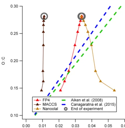
a manner similar to Aiken et al. (2008). There are nine points on each curve, representing points in time during the GECKO-A simulation, with the model predicting a mono-tonic increase in O : C over time. It is worth noting the values are low compared to typical atmospheric LV-OOA (Aiken et al., 2008; Kroll et al., 2011). Overall, use of the FP4 and Nanoolal keys gives absolute f44s that compare well with published calibrations relative to O : C, specifically Aiken et al. (2008) and the updated calibration presented by Cana-garatna et al. (2015). The direction of the trend inf44 ver-sus O : C is reversed when using the Nanoolal keys, withf44 decreasing with O : C, which runs contrary to expectations. However, it should be noted that the values are within the spread of values used to generate the Aiken et al. (2008) and Canagaratna et al. (2015) calibrations, as these performed regressions over much bigger ranges of O : C than obtained in this simulation, so the prediction based on Nanoolal keys could still be plausible.
Figure 8.Comparison of O : C ratios and predicted fractional con-tribution to the AMS m/z44 channel (f44) for the Valorso et al. (2011) GECKO-A simulation, compared against the regressions performed by Aiken et al. (2008) and Canagaratna et al. (2015). The highlighted points indicate the final points in the simulation.
oxygenated functional groups to the molecules that are re-sponsible for both the suppression of vapour pressures nec-essary for SOA formation and also the increase in the f44 metric (Canagaratna et al., 2015). More recent versions of GECKO-A have included such mechanisms (McVay et al., 2016); however, a systematic comparison of the predicted spectra based on these inclusions is beyond the scope of this proof-of-concept paper and will be presented in a future pub-lication.
4 Discussion and future work
The preceding analysis demonstrates the potential for the methodology presented to lead to interesting investigations on model versus measured mass spectra. However, there are a number of remaining improvements that need to be made. It is inevitable that not all of the chemical species predicted by the models will be covered by previous laboratory work. If a class of species predicted by any chemical mechanism is identified as not covered by existing SMARTS-based frag-mentation rules, it could be characterised in the laboratory using the same facilities and methodologies employed for previous characterisation work (Canagaratna et al., 2015, and references therein).
On the sensitivity to choice of fingerprint, our results demonstrate compound specific trends that lead to perfor-mance variability when applied to a complex SOA sys-tem that is not apparent when analysing median cosine an-gle statistics. Combining available fingerprints into one can
Figure 9.“Triangle plot” comparing predictedf44andf43values for the Valorso et al. (2011) GECKO-Aα-pinene SOA simulation with chamber experiments. The Chhabra et al. (2011) data compare different oxidant systems and are taken from Fig. 2a of that paper. The chronological final points in each dataset are highlighted.
slightly improve performance in some cases, but as the com-parison of isolated MACCS versus FP4 performance illus-trates, there is potential danger in overfitting to distinct fea-tures in the training set that is not provided by the box-model output. To re-iterate, one might expect a collection of keys that relate to EI fragmentation principles to offer a more ro-bust basis for fitting any method used here. However, that requires further work with additional laboratory data to vali-date the efficacy of any new bespoke fingerprint.
The methods here have a number of uses, although it must be re-iterated that the predicted mass spectra are not defini-tive. The performance of this method will be improved by the addition of further training data. Following the develop-ment of group contribution methods, this could include stud-ies on compounds within a specific serstud-ies and mixtures of those compounds. As outlined in the Introduction, the ability of this model to predict AMS spectra will be useful in the development and validation of explicit SOA mechanisms in the laboratory, meaning that the models can be challenged by the entire mass spectrum and not just the mass and O : C ratio. This method can also be used at the experiment design stage, allowing predictions of whether an AMS will be able to discern expected changes in composition associated with a process and thus whether it will be useful to test particular hypotheses.
complex-ity associated with atmospheric SOA to (typically) two fac-tors results in an increase in “rotational ambiguity” associ-ated with the factorisation. A two-component factorisation of SOA is often interpreted as representing the “low volatil-ity” and “semivolatile” components of the SOA (Jimenez et al., 2009), although this has shown not to be applicable to all environments, where other sources of variability contribute to the split in the factors (Young et al., 2015). If the mass spectral response to atmospheric SOA could be more explic-itly simulated using this technique, a synthetic AMS dataset could be used as the subject of PMF analysis in a manner similar to Ulbrich et al. (2009). This in turn could be used to investigate the contributions of the factorisation on a more explicit level and investigate the effects this has on rotational ambiguity and the validity of solutions.
Code availability. A publicly available copy of the code used to derive performance statistics of the chosen regression methods can be found at https://github.com/loftytopping/STRAPS covered by a GPL v3.0 license. This includes a copy of the AMS spectral files that now also include appropriate SMILEs strings. The code sepa-rates the four fingerprint libraries used in this study. We also provide an associated DOI for the exact model version given in this paper as provided by the Zenodo service: https://zenodo.org/record/213068# .WFlryyiPD3s (Topping, 2016).
Please note that an extension to the SMARTS libraries in-cluded in UmanSysProp was carried out in this project. To re-view the features extracted for each fingerprint, please refer to the files “FP4.smarts”, “MACCS.smarts”, “nannoolal_primary.smarts”, and “aiomfac_unifac.smarts” included in the directory UMan-SysProp_public/umansysprop/data/.
Author contributions. David Topping conceived the methodology presented and performed the subsequent model development and analysis. James Allan and Rami Alfarra offered expert guided con-straints on evaluating the model results, including selecting the best comparison metrics to use. Bernard Aumont supplied the results from the Valorso et al. (2011) study. All authors contributed to the writing of the manuscript.
Competing interests. The authors declare that they have no conflict of interest.
Acknowledgements. David Topping, James Allan, and Rami Al-farra received funding from the National Centre for Atmospheric Science (NCAS). This work was built on informatics developed under NERC grant NE/H002588/1.
Edited by: A. Archibald
Reviewed by: two anonymous referees
References
Aiken, A. C., DeCarlo, P. F., and Jimenez, J. L.: Elemen-tal analysis of organic species with electron ionization high-resolution mass spectrometry, Anal. Chem., 79, 8350–8358, https://doi.org/10.1021/ac071150w, 2007.
Aiken, A. C., Decarlo, P. F., Kroll, J. H., Worsnop, D. R., Huff-man, J. A., Docherty, K. S., Ulbrich, I. M., Mohr, C., Kim-mel, J. R., Sueper, D., Sun, Y., Zhang, Q., Trimborn, A., Northway, M., Ziemann, P. J., Canagaratna, M. R., Onasch, T. B., Alfarra, M. R., Prevot, A. S. H., Dommen, J., Du-plissy, J., Metzger, A., Baltensperger, U., and Jimenez, J. L.: O/C and OM/OC ratios of primary, secondary, and ambi-ent organic aerosols with high-resolution time-of-flight aerosol mass spectrometry, Environ. Sci. Technol., 42, 4478–4485, https://doi.org/10.1021/es703009q, 2008.
Alfarra, M. R., Good, N., Wyche, K. P., Hamilton, J. F., Monks, P. S., Lewis, A. C., and McFiggans, G.: Water uptake is indepen-dent of the inferred composition of secondary aerosols derived from multiple biogenic VOCs, Atmos. Chem. Phys., 13, 11769– 11789, https://doi.org/10.5194/acp-13-11769-2013, 2013. Aumont, B., Szopa, S., and Madronich, S.: Modelling the
evo-lution of organic carbon during its gas-phase tropospheric ox-idation: development of an explicit model based on a self generating approach, Atmos. Chem. Phys., 5, 2497–2517, https://doi.org/10.5194/acp-5-2497-2005, 2005.
Aumont, B., Valorso, R., Mouchel-Vallon, C., Camredon, M., Lee-Taylor, J., and Madronich, S.: Modeling SOA formation from the oxidation of intermediate volatility n-alkanes, Atmos. Chem. Phys., 12, 7577–7589, https://doi.org/10.5194/acp-12-7577-2012, 2012.
Barley, M. H. and McFiggans, G.: The critical assessment of vapour pressure estimation methods for use in modelling the formation of atmospheric organic aerosol, Atmos. Chem. Phys., 10, 749– 767, https://doi.org/10.5194/acp-10-749-2010, 2010.
Bauer, C. A. and Grimme, S.: How to Compute Electron Ionization Mass Spectra from First Principles, J. Phys. Chem. A, 120, 3755– 3766, https://doi.org/10.1021/acs.jpca.6b02907, 2016.
Bergström, R., Denier van der Gon, H. A. C., Prévôt, A. S. H., Yttri, K. E., and Simpson, D.: Modelling of organic aerosols over Eu-rope (2002–2007) using a volatility basis set (VBS) framework: application of different assumptions regarding the formation of secondary organic aerosol, Atmos. Chem. Phys., 12, 8499–8527, https://doi.org/10.5194/acp-12-8499-2012, 2012.
Bilde, M., Barsanti, K., Booth, M., Cappa, C. D., Donahue, N. M., Emanuelsson, E. U., McFiggans, G., Krieger, U. K., Marcolli, C., Tropping, D., Ziemann, P., Barley, M., Clegg, S., Dennis-Smither, B., Hallquist, M., Hallquist, A. M., Khlystov, A., Kul-mala, M., Mogensen, D., Percival, C. J., Pope, F., Reid, J. P., da Silva, M. A. V. R., Rosenoern, T., Salo, K., Soonsin, V. P., Yli-Juuti, T., Prisle, N. L., Pagels, J., Rarey, J., Zardini, A. A., and Ri-ipinen, I.: Saturation Vapor Pressures and Transition Enthalpies of Low-Volatility Organic Molecules of Atmospheric Relevance: From Dicarboxylic Acids to Complex Mixtures, Chem. Rev., 115, 4115–4156, https://doi.org/10.1021/cr5005502, 2015. Camredon, M., Aumont, B., Lee-Taylor, J., and Madronich, S.:
The SOA/VOC/NOxsystem: an explicit model of secondary
Canagaratna, M. R., Jimenez, J. L., Kroll, J. H., Chen, Q., Kessler, S. H., Massoli, P., Hildebrandt Ruiz, L., Fortner, E., Williams, L. R., Wilson, K. R., Surratt, J. D., Donahue, N. M., Jayne, J. T., and Worsnop, D. R.: Elemental ratio measurements of organic compounds using aerosol mass spectrometry: characterization, improved calibration, and implications, Atmos. Chem. Phys., 15, 253–272, https://doi.org/10.5194/acp-15-253-2015, 2015. Chhabra, P. S., Ng, N. L., Canagaratna, M. R., Corrigan, A.
L., Russell, L. M., Worsnop, D. R., Flagan, R. C., and Se-infeld, J. H.: Elemental composition and oxidation of cham-ber organic aerosol, Atmos. Chem. Phys., 11, 8827–8845, https://doi.org/10.5194/acp-11-8827-2011, 2011.
Drewnick, F., Diesch, J.-M., Faber, P., and Borrmann, S.: Aerosol mass spectrometry: particle–vaporizer interactions and their con-sequences for the measurements, Atmos. Meas. Tech., 8, 3811– 3830, https://doi.org/10.5194/amt-8-3811-2015, 2015.
Ehn, M., Thornton, J. A., Kleist, E., Sipila, M., Junninen, H., Pullinen, I., Springer, M., Rubach, F., Tillmann, R., Lee, B., Lopez-Hilfiker, F., Andres, S., Acir, I. H., Rissanen, M., Joki-nen, T., Schobesberger, S., Kangasluoma, J., KontkaJoki-nen, J., Nieminen, T., Kurten, T., Nielsen, L. B., Jorgensen, S., Kjaer-gaard, H. G., Canagaratna, M., Dal Maso, M., Berndt, T., Petaja, T., Wahner, A., Kerminen, V. M., Kulmala, M., Worsnop, D. R., Wildt, J., and Mentel, T. F.: A large source of low-volatility secondary organic aerosol, Nature, 506, 476–479, https://doi.org/10.1038/nature13032, 2014.
Gasteiger, J., Hanebeck, W., and Schulz, K. P.: Prediction of Mass-Spectra from Structural Information, J. Chem. Inf. Comp. Sci., 32, 264–271, https://doi.org/10.1021/Ci00008a001, 1992. Hallquist, M., Wenger, J. C., Baltensperger, U., Rudich, Y.,
Simp-son, D., Claeys, M., Dommen, J., Donahue, N. M., George, C., Goldstein, A. H., Hamilton, J. F., Herrmann, H., Hoff-mann, T., Iinuma, Y., Jang, M., Jenkin, M. E., Jimenez, J. L., Kiendler-Scharr, A., Maenhaut, W., McFiggans, G., Mentel, Th. F., Monod, A., Prévôt, A. S. H., Seinfeld, J. H., Surratt, J. D., Szmigielski, R., and Wildt, J.: The formation, properties and im-pact of secondary organic aerosol: current and emerging issues, Atmos. Chem. Phys., 9, 5155–5236, https://doi.org/10.5194/acp-9-5155-2009, 2009.
Hamilton, J. F., Baeza-Romero, M. T., Finessi, E., Rickard, A. R., Healy, R. M., Peppe, S., Adams, T. J., Daniels, M. J. S., Ball, S. M., Goodall, I. C. A., Monks, P. S., Borras, E., and Munoz, A.: Online and offline mass spectrometric study of the impact of oxidation and ageing on glyoxal chemistry and uptake onto ammonium sulfate aerosols, Faraday Discuss., 165, 447–472, https://doi.org/10.1039/c3fd00051f, 2013.
Jimenez, J. L., Canagaratna, M. R., Donahue, N. M., Prevot, A. S. H., Zhang, Q., Kroll, J. H., DeCarlo, P. F., Allan, J. D., Coe, H., Ng, N. L., Aiken, A. C., Docherty, K. S., Ulbrich, I. M., Grieshop, A. P., Robinson, A. L., Duplissy, J., Smith, J. D., Wil-son, K. R., Lanz, V. A., Hueglin, C., Sun, Y. L., Tian, J., Laak-sonen, A., Raatikainen, T., Rautiainen, J., Vaattovaara, P., Ehn, M., Kulmala, M., Tomlinson, J. M., Collins, D. R., Cubison, M. J., Dunlea, E. J., Huffman, J. A., Onasch, T. B., Alfarra, M. R., Williams, P. I., Bower, K., Kondo, Y., Schneider, J., Drewnick, F., Borrmann, S., Weimer, S., Demerjian, K., Salcedo, D., Cot-trell, L., Griffin, R., Takami, A., Miyoshi, T., Hatakeyama, S., Shimono, A., Sun, J. Y., Zhang, Y. M., Dzepina, K., Kimmel, J. R., Sueper, D., Jayne, J. T., Herndon, S. C., Trimborn, A.
M., Williams, L. R., Wood, E. C., Middlebrook, A. M., Kolb, C. E., Baltensperger, U., and Worsnop, D. R.: Evolution of Or-ganic Aerosols in the Atmosphere, Science, 326, 1525–1529, https://doi.org/10.1126/science.1180353, 2009.
Kroll, J. H., Donahue, N. M., Jimenez, J. L., Kessler, S. H., Cana-garatna, M. R., Wilson, K. R., Altieri, K. E., Mazzoleni, L. R., Wozniak, A. S., Bluhm, H., Mysak, E. R., Smith, J. D., Kolb, C. E., and Worsnop, D. R.: Carbon oxidation state as a metric for describing the chemistry of atmospheric organic aerosol, Nat. Chem., 3, 133–139, https://doi.org/10.1038/NCHEM.948, 2011. Laaksonen, A., Kulmala, M., O’Dowd, C. D., Joutsensaari, J., Vaat-tovaara, P., Mikkonen, S., Lehtinen, K. E. J., Sogacheva, L., Dal Maso, M., Aalto, P., Petäjä, T., Sogachev, A., Yoon, Y. J., Lihavainen, H., Nilsson, D., Facchini, M. C., Cavalli, F., Fuzzi, S., Hoffmann, T., Arnold, F., Hanke, M., Sellegri, K., Umann, B., Junkermann, W., Coe, H., Allan, J. D., Alfarra, M. R., Worsnop, D. R., Riekkola, M.-L., Hyötyläinen, T., and Vi-isanen, Y.: The role of VOC oxidation products in continen-tal new particle formation, Atmos. Chem. Phys., 8, 2657–2665, https://doi.org/10.5194/acp-8-2657-2008, 2008.
McLafferty, F. T.: Interpretation of mass spectra, edited by: Vetter, W., University Science Books, Mill Valley, California, 1994. McVay, R. C., Zhang, X., Aumont, B., Valorso, R., Camredon, M.,
La, Y. S., Wennberg, P. O., and Seinfeld, J. H.: SOA formation from the photooxidation of a-pinene: systematic exploration of the simulation of chamber data, Atmos. Chem. Phys., 16, 2785– 2802, https://doi.org/10.5194/acp-16-2785-2016, 2016. Morgan, W. T., Allan, J. D., Bower, K. N., Highwood, E. J., Liu,
D., McMeeking, G. R., Northway, M. J., Williams, P. I., Krejci, R., and Coe, H.: Airborne measurements of the spatial distribu-tion of aerosol chemical composidistribu-tion across Europe and evolu-tion of the organic fracevolu-tion, Atmos. Chem. Phys., 10, 4065–4083, https://doi.org/10.5194/acp-10-4065-2010, 2010.
Murphy, D. M.: The effects of molecular weight and ther-mal decomposition on the sensitivity of a therther-mal desorption aerosol mass spectrometer, Aerosol Sci. Tech., 50, 118–125, https://doi.org/10.1080/02786826.2015.1136403, 2016. Nannoolal, Y., Rarey, J., and Ramjugernath, D.: Estimation of pure
component properties – Part 3. Estimation of the vapor pres-sure of non-electrolyte organic compounds via group contribu-tions and group interaccontribu-tions, Fluid Phase Equilibr., 269, 117– 133, https://doi.org/10.1016/j.fluid.2008.04.020, 2008.
Ng, N. L., Canagaratna, M. R., Jimenez, J. L., Chhabra, P. S., Se-infeld, J. H., and Worsnop, D. R.: Changes in organic aerosol composition with aging inferred from aerosol mass spectra, At-mos. Chem. Phys., 11, 6465–6474, https://doi.org/10.5194/acp-11-6465-2011, 2011.
Noziere, B., Kaberer, M., Claeys, M., Allan, J., D’Anna, B., Decesari, S., Finessi, E., Glasius, M., Grgic, I., Hamil-ton, J. F., Hoffmann, T., Iinuma, Y., Jaoui, M., Kahno, A., Kampf, C. J., Kourtchev, I., Maenhaut, W., Marsden, N., Saarikoski, S., Schnelle-Kreis, J., Surratt, J. D., Szidat, S., Szmigielski, R., and Wisthaler, A.: The Molecular Identi-fication of Organic Compounds in the Atmosphere: State of the Art and Challenges, Chem. Rev., 115, 3919–3983, https://doi.org/10.1021/cr5003485, 2015.
An open chemical toolbox, J. Cheminformatics, 3, 33, https://doi.org/10.1186/1758-2946-3-33, 2011.
Pedregosa, F., Varoquaux, G., Gramfort, A., Michel, V., Thirion, B., Grisel, O., Blondel, M., Prettenhofer, P., Weiss, R., Dubourg, V., Vanderplas, J., Passos, A., Cournapeau, D., Brucher, M., Per-rot, M., and Duchesnay, E.: Scikit-learn: Machine Learning in Python, J. Mach. Learn. Res., 12, 2825–2830, 2011.
Putta, S., Eksterowicz, J., Lemmen, C., and Stanton, R.: A novel subshape molecular descriptor, J. Chem. Inf. Comp. Sci., 43, 1623–1635, https://doi.org/10.1021/ci0256384, 2003.
Robinson, A. L., Donahue, N. M., Shrivastava, M. K., Weitkamp, E. A., Sage, A. M., Grieshop, A. P., Lane, T. E., Pierce, J. R., and Pandis, S. N.: Rethinking organic aerosols: Semivolatile emissions and photochemical aging, Science, 315, 1259-1262, 10.1126/science.1133061, 2007.
Robinson, E. S., Donahue, N. M., Ahern, A. T., Ye, Q., and Lipsky, E.: Single-particle measurements of phase partitioning between primary and secondary organic aerosols, Faraday Discuss., 189, 31–49, https://doi.org/10.1039/c5fd00214a, 2016.
Ruske, S., Topping, D. O., Foot, V. E., Kaye, P. H., Stanley, W. R., Crawford, I., Morse, A. P., and Gallagher, M. W.: Evalua-tion of machine learning algorithms for classificaEvalua-tion of primary biological aerosol using a new UV-LIF spectrometer, Atmos. Meas. Tech., 10, 695–708, https://doi.org/10.5194/amt-10-695-2017, 2017.
Saunders, S. M., Jenkin, M. E., Derwent, R. G., and Pilling, M. J.: World Wide Web site of a Master Chemical Mechanism (MCM) for use in tropospheric chemistry models, Atmos. Environ., 31, 1249–1249, https://doi.org/10.1016/S1352-2310(97)85197-7, 1997.
Sipila, M., Sarnela, N., Jokinen, T., Henschel, H., Junninen, H., Kontkanen, J., Richters, S., Kangasluoma, J., Franchin, A., Per-akyla, O., Rissanen, M. P., Ehn, M., Vehkamaki, H., Kurten, T., Berndt, T., Petaja, T., Worsnop, D., Ceburnis, D., Kerminen, V. M., Kulmala, M., and O’Dowd, C.: Molecular-scale evidence of aerosol particle formation via sequential addition of HIO3, Na-ture, 537, 532–534, https://doi.org/10.1038/nature19314, 2016. Spracklen, D. V., Jimenez, J. L., Carslaw, K. S., Worsnop, D. R.,
Evans, M. J., Mann, G. W., Zhang, Q., Canagaratna, M. R., Allan, J., Coe, H., McFiggans, G., Rap, A., and Forster, P.: Aerosol mass spectrometer constraint on the global secondary organic aerosol budget, Atmos. Chem. Phys., 11, 12109–12136, https://doi.org/10.5194/acp-11-12109-2011, 2011.
Topping, D.: loftytopping/STRAPS: STRAPS v1.0, Zenodo, https://doi.org/10.5281/zenodo.213068, 2016.
Topping, D., Barley, M., Bane, M. K., Higham, N., Aumont, B., Dingle, N., and McFiggans, G.: UManSysProp v1.0: an online and open-source facility for molecular property prediction and atmospheric aerosol calculations, Geosci. Model Dev., 9, 899– 914, https://doi.org/10.5194/gmd-9-899-2016, 2016.
Ulbrich, I. M., Canagaratna, M. R., Zhang, Q., Worsnop, D. R., and Jimenez, J. L.: Interpretation of organic components from Posi-tive Matrix Factorization of aerosol mass spectrometric data, At-mos. Chem. Phys., 9, 2891–2918, https://doi.org/10.5194/acp-9-2891-2009, 2009.
Valorso, R., Aumont, B., Camredon, M., Raventos-Duran, T., Mouchel-Vallon, C., Ng, N. L., Seinfeld, J. H., Lee-Taylor, J., and Madronich, S.: Explicit modelling of SOA for-mation from a-pinene photooxidation: sensitivity to vapour pressure estimation, Atmos. Chem. Phys., 11, 6895–6910, https://doi.org/10.5194/acp-11-6895-2011, 2011.
Volkamer, R., Jimenez, J. L., San Martini, F., Dzepina, K., Zhang, Q., Salcedo, D., Molina, L. T., Worsnop, D. R., and Molina, M. J.: Secondary organic aerosol formation from anthropogenic air pollution: Rapid and higher than expected, Geophys. Res. Lett., 33, L17811, https://doi.org/10.1029/2006gl026899, 2006. Young, D. E., Allan, J. D., Williams, P. I., Green, D. C., Harrison,
R. M., Yin, J., Flynn, M. J., Gallagher, M. W., and Coe, H.: In-vestigating a two-component model of solid fuel organic aerosol in London: processes, PM1 contributions, and seasonality, At-mos. Chem. Phys., 15, 2429–2443, https://doi.org/10.5194/acp-15-2429-2015, 2015.