Issues
ISSN: 2146-4138
available at http: www.econjournals.com
International Journal of Economics and Financial Issues, 2017, 7(4), 15-22.
Has Financialization in Commodity Markets Affected the
Predictability in Metal Markets? The Efficient Markets
Hypotheses for Metal Returns
Lya Paola Sierra
1*, Luis Eduardo Girón
2, Carolina Osorio
31Department of Economics, Pontificia Universidad Javeriana, Calle 18 No. 118-250 Av. Cañasgordas, Cali, Colombia, 2Department of Economics, Pontificia Universidad Javeriana, Colombia, 3Energy Planning Office, Emcali E.I.C.E. Colombia. *Email: [email protected]
ABSTRACT
This article evaluates the hypothesis that returns of metal prices are unpredictable (i.e., under the weak form efficient market hypothesis). The possible effect that financialization in the commodity market has had in the predictability of this is also evaluated. Using statistical techniques such as the portmanteau test, the variance ratio test, and a robustness test on the monthly returns of metals for the 1992-2015 period, it is found that the market of some metals is persistently inefficient whereas others fluctuate between periods of efficiency and inefficiency. There is no clear effect of financialization on the efficiency of the metal market.
Keywords: Efficient Markets Hypotheses, Metal Prices, Forecasting
JEL Classifications: C12, E39, F00, G14, Q02
1. INTRODUCTION
In economics, it is common to discuss supply and demand as determinants of the prices of different types of goods, including raw materials. However, the records on changes in the prices of different commodities do not necessarily correspond to changes
in these economic variables. In fact, for some authors, such as
Olson et al. (2014), not only have commodity markets been more volatile in recent years, but also the cycle of raw materials prices has an interesting similarity to the price cycles in the United States
stock market, as shown in Figure 1.
This behavior of prices has led to the assumption that other
factors, such as speculation, are playing an increasing role in the determination of commodity prices. For some authors, such as Büyüksahin and Robe (2013), Silvennoinen and Thorp (2013), Wray (2008), and Hong and Yogo (2012), this increase in speculation in the commodity market is due to a phenomenon called “financialization.” Financialization involves the entry of new players into the market, such as mutual funds and pensions from
2004 onwards, and the overwhelming increase in the acquisition of commodity futures, which are viewed only as financial assets
that are suitable for reducing the portfolios volatility and risk. According to the above, financialization has made it possible for some commodity markets to be deeper, given the greater number of players in the market and the greater number of speculative transactions. This fact can lead to an increase in the flow of
information available to all market participants and, therefore, can
convert the market of some commodities into efficient markets.
This article aims to test the weak form of efficient markets hypotheses (EMH) on the group of metals composed of aluminium, copper, lead, nickel, tin, uranium, and zinc by evaluating the periods before and after financialization. The purpose of this article is to determine which of these raw materials have efficient and inefficient behavior and whether financialization is a determining factor of the changes in the efficiency of these markets.
(Fama, 1970. p. 383). Additionally, the definition from Fama can be interpreted as a random process that behaves as a fair game, whose results cannot be systematically predicted (Uribe and Ulloa, 2011, p. 2). Therefore, it can be assumed that increasingly speculative behaviour and a greater number of transactions may make it difficult to predict the prices of these metals.
Although many economic studies have focused on the application of tools for predicting the prices of different raw materials (e.g., Chinn and Cobion, 2015, Poncela et al., 2014), there are few studies that are concerned with the evaluation of the efficiency of these markets. Most papers have focused on evaluating the EMH on the stock markets (i.e., Campbell et al., 1997; Cochrane, 2001).
Among the few studies that are concerned with measuring the efficiency of commodities markets is the study by He and Holt (2004) in the case of forestry raw materials. These authors implement a Generalized Quadratic ARCH model on weekly prices between June 1997 and October 2001 for the following
commodities: Softwood, oriented strand board, and bleached
softwood; they find that the three markets studied are inefficient. On the other hand, Inoue and Hamori (2012) study the efficiency of commodity futures in India using the fully modified minimized squares model. Their results indicate that there is only efficiency in the subsample of the year 2009 for the indices evaluated. Finally, Kristoufek and Vosvrda (2014) take 25 agricultural, energy, metals, and grains commodities to test efficiency in futures markets. The results show that the most efficient markets are those for heated oil, crude oil, and cotton. In general, it is estimated that the most efficient raw materials are energy whereas the least efficient are agricultural.
The importance of studying the metal markets lies in the fact that metals are generally an important input in industrial production; thus, the evolution of these markets is highly related to economic cycles (see, i.e., Labys et al., 1999). According to authors such as Issler et al. (2014), the demand for metals comes from not only developed countries, but also from emerging countries such as China, in which industrial activity has become an important focus
of economic activity. In addition, no studies have been conducted to determine the effects of financialization as a potential causal factor for changes in the efficiency of commodity markets, which constitutes an additional argument for this study’s importance and novelty.
This article is composed of three sections in addition to this
introduction. In the second section, data and methodology is presented. This section presents the main elements of efficient market theory and outlines the three statistical techniques used in the present study to test weak efficiency in the metal market.
The third section presents the results obtained in relation to
the efficiency tests. The last section presents the most relevant
conclusions of the research and some recommendations.
2. METHODOLOGY
2.1. Data
The data used correspond to the price series per metric ton of seven
raw materials that are categorized as metals in the International Monetary Fund (IMF) database. These are aluminium, copper, lead, nickel, tin, uranium, and zinc. The frequency of the data is monthly, comprising the period from January 1992 to December 2015.
The total sample was divided into two subsamples, with
the comparison period being the period before and after financialization. For some authors, the increase in speculation in the commodity market due to the entry of new participants into the market dates from the end of 2003 (e.g., Masters, 2008; Tang and Xiong, 2012), and an increase has been noted in the co-movement between commodity prices since 2004 (as described by Poncela et al., 2014). Therefore, for the pre-financialization period, a subsample that starts in January 1992 and lasts until December 2003 is formed. For the post-financialization period, the second subsample begins in January 2004 and lasts until December 2015.
Each of the subsamples has a series of prices of 144 data in total.
2.2. The Concept of Efficient Markets
The concept of efficiency is associated with the following question: Is it possible to predict the return on assets (ROA)? From the EMH (Fama, 1970), ROAs are not predictable if the prices of these
assets correctly reflect the available information. Malkiel (1992) broadens the previous definition because he links the concept of efficiency to sets of information. In this sense, a market is efficient if the prices of assets are not altered when revealing the information to all of the agents participating in the market. Therefore, it is not possible to make profits with such information. Fama (1970), following Mankiel (1992), classify market efficiency in three ways: Weak, semi-strong, and strong.
Weak efficiency occurs when the information set consists only of historical price information, whereas semi-strong efficiency
occurs when the information set consists of all available public information, such as announcements about the division of shares,
annual reports, and others. Finally, strong efficiency is presented when the information set is constituted by all of the information susceptible to being known, e.g., private or privileged information
of a monopolistic character.
Source: Authors, with data from the International Monetary Fund and Chicago Board Options Exchange (CBOE), Note: Normalized data
In this study, we use the concept of weak efficiency because it is based on only the historical series of the seven metals provided by the IMF.
Weak efficiency is tested by the random walk test, which essentially follows the structure below:
pt = µ + pt-1 + εt (1)
where pt is the logarithm of the price at time t, pt-1is the logarithm of the price at time t-1, µ is the expected drift or change in price, and εtis the error term or disturbance. A characteristic of these
processes is that prices follow random structures, which makes it
impossible to predict their future values and so that the expected returns will be equal to zero, meaning that the best prediction of the price at time t will be equal to the price at time t-1. Therefore, if one of the tests does not reject the random walk hypothesis, then the indication would be that the market behaves efficiently
and future prices will therefore not be predictable.
Random walks are divided into three types according to the manner in which εt is distributed. Random walk 1 consists of independent and identically distributed processes; random walk 2 follows an independent but not identically distributed process; and random walk 3 does not fulfil any of the above characteristics, but the covariance of value t and lag value t-k is equal to zero. Each of these types of random walks possesses a particular set of empirical tests to be verified, in which one typically works with continually compounded price returns. In this study, the random walk 3 tests are implemented, specifically the portmanteau statistic and the
variance ratio test, which are described below.
2.3. Efficiency Tests
The present study is based on the concept of weak efficiency and some statistical techniques for determining whether a specific market is efficient, such as the portmanteau statistic and the
variance ratio test. To evaluate the robustness of our results, we
proposed to compare the predictive capacity of an univariate ARMA model against a random walk model. With this, we aim to explore the predictability of metals prices returns measured on a monthly basis. Our measure of forecasting performance is the out-of-sample root mean square error of prediction (RMSE) for
one-step-ahead forecasts.
2.4. Portmanteau Statistic
In this test, the set of information is the historical series of asset
prices, and two options can be used: The statistic from Box and Pierce (1970), which is presented in equation (2), or the statistic from Ljung and Box (1978), which is associated with equation (3). The Ljung-Box statistic provides a better fit for small samples, which is why it is the most frequently used.
m 2 m
k=1
Box Pierce (Q ) = T −
∑
ρ (k) (2)′m m 2
k=1
(K) Ljung Box (Q ) = T (T + 2)
T - K
ρ
−
∑
(3)The null hypothesis is that all autocorrelations from 1 to m are equal to zero, and the alternative hypothesis is that at least one
of the autocorrelations is different from zero. Therefore, if this hypothesis is rejected, then the random walk and, therefore, market efficiency are discarded.
H0: ρ1 = ρ2 = ρ3 = ρk = 0 H1: at least one ρk is ≠ 0 (4)
2.5. Variance Ratio Test
The variance ratio test is a test for determining whether the prices
of an asset are predictable. Lo and Mackinlay (1988, 1989) developed this test, which is based on a property common to the different types of random walks in that the variance of random
walk increments must be a linear function of the time interval
(Campbell et al., 1997). Therefore, this test evaluates the rate between the variance of a continuously compound return over a
period of time and the variance of the same return over a period
of time q, in which if a random walk process is followed, then the variance ratio must be equal to 1, regardless of the number of lags. Accordingly, the variance ratio VR(q) is given by equation (5):
VR var rt
q var rt
q q k
q k
k q
( )
≡ [ ( )]= +∑
=− − ρ. [ ] ( )( ) ( )
( )
1 2 1
1 1
(5)
Where ρ(k) corresponds to the k-th order of the autocorrelation coefficient of rt. The variance ratio is not necessarily exactly equal to 1, which is why the statistic of equation (6) can prove its significance:
Ψ ≡
θ
*
( )
q nq VR( ( )q −1) (6)According to the level of significance chosen, if the value of the statistic ᴪ*(q) falls outside the range of acceptance, we can reject the random walk hypothesis and, therefore, market efficiency.
2.6. Robustness Test
In addition to the tests noted above, we proposed a robustness
check to evaluate the predictability of metal returns. Apart from the a random walk model, we use a univariate ARMA model for prices in logs which takes into account outliers estimated automatically, using Gómez and Maravall (1996)’s TRAMO program (Time series Regression with ARIMA noise, Missing values and Outliers), which follows the specification:
i i,t it
i
(B)
lnP = +outliers
f (B)
θ ε
∆ , where ϕi(B) and ϕi(B) are autoregresive and moving average polynomials of order pi and qi respectively on the backshift operator B, and ∆ is the difference operator (1−B)1.
Our procedure in analyzing the data is as follows:
1. We estimate the random walk and univariate ARMA model for the both subperiods (pre and post-finacializacion). 2. We generate one-step-ahead forecasts. For the first sub-period
we start our out-of-sample forecasts in 2001:1, and for the second su-period we start in 2013:1, re-estimate the models adding one data point at the time. In other words, we use an expanding window of 3 years.
3. We compute the RMSE for each model to assess its forecasting
performance.
4. We compare the RMSE of ARMA model with that of the random walk by means of the following ratio:
RMSE
RMSE
ARMA
Random Walk
i
j
If this ratio is greater than one, then it is concluded that the market is efficient because the monthly predictions of the random walk
are better than those of the univariate model. If the ratio between
the RMSE of the univariate model and the RMSE of the random walk is less than one, then the market is inefficient because the
predictions of the univariate model surpass the naive predictions of the random walk. In addition we compare the predictive content
for every model in both of the periods (pre-2004 and post-2004).
3. ANALYSIS OF THE RESULTS
3.1. Descriptive Analysis of the Information Used
Figure 2 shows the graph of prices at the level of each of the variables. In this graph, with the exception of aluminium, periods of price stability can be observed up to 2004; after this date, there are periods of great variations in prices2. The descriptive statistics of the series for the first and second subsample are presented in
Table 1. In these, we can observe an increase in the coefficient
of variation in the second period, which can be interpreted as a
measure of the increased volatility of metal prices. The coefficient of variation with the greatest increase is uranium, which changes from a coefficient of variation of 20.15% in the pre-financialization period to a coefficient of 45.50% in the post-financialization period, which makes it the metal with the greatest increase in volatility.
In this study, the returns of metal prices are used. Therefore, the data are transformed by applying the logarithm to the difference
between the price in period t and the price in t-1, such that:
rt = pt – pt-1 (7)
where rt are returns of prices of metals, pt represents the logarithm
of prices at t, and pt-1 represents the logarithm of prices at pt-1.
3.2. Results of the Efficiency Tests on the Seven
Selected Metals
Although there is a series of criticisms about the tests used because they do not incorporate dynamics within their structure, which does not allow us to measure the dynamics of the informational efficiency of a given market, the presented results are valid because only two periods are considered, i.e., before and after financialization, thereby incorporating the possible changes in terms of efficiency that can be presented in the metal market.
2 Tests were performed to determine structural breakage in the series. Specifically, the Quandt-Andrews test (1960) was applied, and structural breakpoints in the period of the global economic crisis from 2007 to 2008 and for some metals in 2011 were shown. Appendix 1 presents the results of the test.
Table 2 presents the results of the Portmanteau Ljung-Box
Statistical test and the variance ratio test for the period prior
to financialization. According to the portmanteau statistic, the hypothesis that there is no autocorrelation is rejected; that is, the random walk hypothesis for aluminium, copper, lead and nickel is rejected, at the confidence levels of 5% and 10%. In comparison, tin, uranium, and zinc do not reject the random walk hypothesis.
The results of the variance ratio test for the period prior to
financialization indicate that the only raw material of the group of metals studied that does not reject the random walk hypothesis is uranium whereas the other metals reject this hypothesis at the confidence levels of 5% and 10%.
Table 3 presents the results for the random walk tests corresponding
to the second subsample, i.e., the period in the presence of
financialization. The results indicate that lead is the only metal that does not reject the random walk hypothesis in the second subsample. The variance ratio test for the period from January 2004 to December 2015 rejects the random walk hypothesis for all metals, at both levels of significance.
Table 4 shows the results of the tests in both periods and in terms
of efficiency. According to the portmanteau statistic, aluminium, copper, and nickel remain inefficient in the entire sample, such that financialization is not interpreted as a possible factor of change for these metals. On the other hand, lead went from being inefficient to efficient, whereas tin, uranium, and zinc present a shift from efficient to inefficient.
According to the variance ratio test in Table 4 in the period prior to
financialization, uranium is the only metal that presents evidence of market efficiency. Once the representative subsample of the post-financialization stage was evaluated, it is indicated that none of the metals is efficient.
Given that efficiency is not found for any metals in the period after financialization, we identify the generating process of each
of these data series so that their future values can be predicted.
Appendix 2 shows the generating process identified for each of
the data series.
Based on the generating process identified, we estimate the forecast for the period 2015M7-2015M12. To validate the accuracy of the forecasts, we calculated the mean absolute percentage error (MAPE). The results of the MAPE are presented in Table 5, in which rows (2) to (7) show the absolute value of the difference between the actual value and the predicted value, divided by the actual value. Finally, row (8) presents the MAPE associated with each metal. From these results, it can be observed that the metal with the highest absolute percentage error was zinc, at 18.28%, constituting the prediction
that deviated the most from the real value, whereas the most reliable
forecast was obtained by tin, with a MAPE of 2.69%. However, it can be said that, in general terms, all of the forecasts obtained results that are very close to the real values and with low percentage errors.
3.3. Robustness Tests
Figure 2: Prices at level, January 1992-December 2015
Source: Authors, with data from the International Monetary Fund
Table 2: Portmanteau statistics and variance ratio for subsample I, January 1992-December 2003
Commodity Portmanteau statistic Variance ratio
Lag 36 Level of significance Joint variation test Level of significance
Q P value 5% 10% Max |z| P value 5% 10%
Aluminium 52.89 0.03 Rejects Rejects 4.15 0.00 Rejects Rejects
Copper 80.64 0.00 Rejects Rejects 3.38 0.00 Rejects Rejects
Lead 47.65 0.09 Rejects* Rejects 3.90 0.00 Rejects Rejects
Nickel 67.12 0.00 Rejects Rejects 3.97 0.00 Rejects Rejects
Tin 41.74 0.24 Does not reject Does not reject 3.71 0.00 Rejects Rejects
Uranium 42.22 0.22 Does not reject Does not reject 2.11 0.13 Does not reject Does not reject
Zinc 41.38 0.25 Does not reject Does not reject 3.48 0.00 Rejects Rejects
*Rejects null hypothesis at 9%
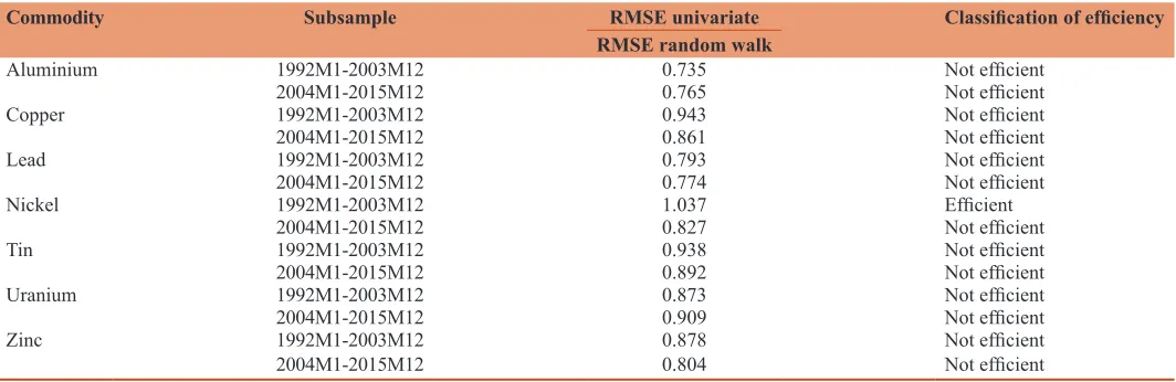
presents the results of the ratios between the RMSE of the ARMA
model and the random walk model forecast for each sub-sample. The last column gives a classification between whether it is efficient or not, based on the assumption that if a variable presents a smaller
Table 1: Descriptive statistics for subsamples I (January 1992-December 2003) and II (January 2004-December 2015)
Statistics per subsample Aluminium Copper Lead Nickel Tin Uranium Zinc
Metal subsample I
Mean (USD/ton) 1440.22 1997.21 537.64 6912.32 5377.66 23111.41 1024.70
Minimum (USD/ton) 1040.02 1377.38 376.34 3865.76 3698.37 15652.80 748.81
Maximum (USD/ton) 2059.36 3076.45 840.98 14185.21 6980.50 36376.23 1650.63
Coefficient of variation (%) 13.39 22.42 19.70 23.70 13.42 20.15 16.77
Metal subsample II
Mean (USD/ton) 2087.85 6379.82 1847.67 19310.09 16580.08 103557.03 2066.37
Minimum (USD/ton) 1338.06 2421.48 747.03 8707.79 6173.72 32628.376 976.80
Maximum (USD/ton) 3067.46 9880.94 3722.61 51783.33 32347.69 300318.23 4381.45
prediction error with the random walk than with a univariate model
forecast, then it can be assumed to be an efficient process. Results
in Table 6 show that nickel in the period prior to financialization
is the only raw material with an efficient behaviour. These results agree with the data in the three random walk tests, in which, in general terms, no efficiencies in the series of returns are observed.
Table 3: Portmanteau statistics and variance ratio for subsample II, January 2004-December 2015
Materia prima Portmanteau statistic Variance ratio
Lag 36 Level of significance Joint test for q>1 Level of significance
Q P value 5% 10% Max |z| P value 5% 10%
Aluminium 79.74 0.00 Rejects Rejects 4.37 0.00 Rejects Rejects
Copper 69.60 0.00 Rejects Rejects 2.78 0.02 Rejects Rejects
Lead 46.80 0.11 Does not reject Does not reject 3.34 0.00 Rejects Rejects
Nickel 64.39 0.00 Rejects Rejects 3.83 0.00 Rejects Rejects
Tin 60.68 0.01 Rejects Rejects 4.62 0.00 Rejects Rejects
Uranium 65.32 0.00 Rejects Rejects 2.39 0.07 Rejects* Rejects
Zinc 73.82 0.00 Rejects Rejects 3.59 0.00 Rejects Rejects
*Rejects null hypothesis at 7%
Table 4: Classification of efficiency pre‑ and post‑financialization with the portmanteau statistic and variance ratio test
Commodity Portmanteau Variance ratio
Pre‑financialization January 1992- December 2003
Post‑financialization January 2004- December 2015
Pre‑financialization January 1992- December 2003
Post‑financialization January 2004- December 2015
Aluminium Not efficient Not efficient Not efficient Not efficient
Copper Not efficient Not efficient Not efficient Not efficient
Lead Not efficient Efficient Not efficient Not efficient
Nickel Not efficient Not efficient Not efficient Not efficient
Tin Efficient Not efficient Not efficient Not efficient
Uranium Efficient Not efficient Efficient Not efficient
Zinc Efficient Not efficient Not efficient Not efficient
Table 5: MAPE of the data forecasted for the periods of 2015M7-2015M12
Period Aluminium Copper Lead Nickel Tin Uranium Zinc
2015M7 0.01 0.01 0.03 0.07 0.01 0.03 0.00
2015M8 0.06 0.10 0.07 0.13 0.02 0.05 0.10
2015M9 0.04 0.06 0.09 0.13 0.04 0.03 0.17
2015M10 0.09 0.08 0.07 0.04 0.06 0.03 0.18
2015M11 0.12 0.17 0.14 0.11 0.01 0.07 0.29
2015M12 0.10 0.23 0.09 0.12 0.01 0.10 0.34
MAPE (%) 6.97 10.90 8.11 10.04 2.69 4.97 18.28
MAPE: Mean absolute percentage error
Table 6: Robustness test, the ratio between the root mean square error of the ARMA forecast and random walk model for a 36-month moving window
Commodity Subsample RMSE univariate Classification of efficiency
RMSE random walk
Aluminium 1992M1-2003M12 0.735 Not efficient
2004M1-2015M12 0.765 Not efficient
Copper 1992M1-2003M12 0.943 Not efficient
2004M1-2015M12 0.861 Not efficient
Lead 1992M1-2003M12 0.793 Not efficient
2004M1-2015M12 0.774 Not efficient
Nickel 1992M1-2003M12 1.037 Efficient
2004M1-2015M12 0.827 Not efficient
Tin 1992M1-2003M12 0.938 Not efficient
2004M1-2015M12 0.892 Not efficient
Uranium 1992M1-2003M12 0.873 Not efficient
2004M1-2015M12 0.909 Not efficient
Zinc 1992M1-2003M12 0.878 Not efficient
2004M1-2015M12 0.804 Not efficient
4. CONCLUSIONS
This paper aimed to test the hypothesis of weak efficiency for a group of metals composed of aluminium, copper, tin, lead, nickel, uranium, and zinc, using as a point of comparison the year 2004 to determine whether financialization is a determining factor in the efficiency of this commodity market. To that end, we mainly
used tests for random walk3, specifically the portmanteau statistic and the variance ratio test. We aim to evaluate the predictability
of the returns of metals.
Based on the theory of Fama (1970) concerning informational efficiency, the question of whether metals have efficient behaviour emerged. Moreover, it was hypothesized that the financialization initiated in 2004, by allowing more players to enter into the stock market, could encourage markets that were not efficient to become efficient due to an increase in information for participants.
First, the results indicate that prior to financialization, there is a certain stability in the prices of the raw materials studied and that, after 2004, all have increases in price volatility, reaching a 25.35% increase in the case of uranium. This result may be due to an increase in speculation caused by multiple players in the market or by the periods of financial crisis that occurred around the year 2008. The high price volatility can be explained by a factor of uncertainty that generated the high purchase and sale of raw materials through future negotiations, supporting the hypothesis that commodities are often viewed as a tool to hedge against risk.
The two tests used from random walk 3 almost consistently indicate inefficiencies throughout the subsamples. First, the
portmanteau statistic indicates that aluminium, copper, and
nickel are inefficient in the entire sample, i.e., between 1992 and 2015, which means that the effects on these raw materials cannot be attributed to financialization. According to the portmanteau results, lead becomes efficient after financialization, the only result coinciding with the initial hypothesis that financialization can make inefficient markets efficient. Contrary to the hypothesis presented, tin, uranium, and zinc go from being efficient to inefficient. Second, the variance ratio test for uranium finds a change from efficient to inefficient, such as with the portmanteau statistic, whereas for the other metals, there are no efficiencies observed throughout the sample.
The two tests agree that uranium goes from being an efficient
market, and therefore not predictable, to being a predictable
raw material, i.e., inefficient. They also agree that, in the post-financialization period, with the exception of lead (according to the portmanteau result), all metals are inefficient, which also occurs mostly in the first subsample. These results can support theories contrary to those of market efficiency, such as information asymmetry, in which market efficiency can occur only under exceptional cases.
Similarly, the high exchange of these metals and the theory that they are negotiated as instruments for risk protection can generate an interest among market participants in accessing insider information, which is addressed by the strong efficiency theory
and which has signalled the impossibility of being in a real market. Therefore, not only because it is an interest in the acquisition of the raw material for its consumption but also because it benefits
those who deal in the stock market, each metal will be treated
as a financial asset, and it will be able to incentivize negotiators
to resort to mechanisms that allow them to know in advance the
price of the metal in the stock market, also leading to the market’s inefficiency.
Regarding the robustness check, they provide evidence in two senses: On the one hand, they allow us to observe whether the predictions generated by a univariate model present a greater
or lesser error than a random walk prediction, in which the best
forecast is the value from the immediately prior period. On the other hand, analysing which of the two methods generates better predictions is an indicator of market efficiency, in the sense that if variables are better predicted by a random walk, then they can be categorized as efficient. The results show that the metals present better forecasts through univariate models than through a random walk, which means that, in general terms, no efficiencies are found, thus agreeing with the results obtained by the portmanteau statistic
and the variance ratio.
REFERENCES
Box, G.E., Pierce, D.A. (1970), Distribution of residual autocorrelations in autoregressive-integrated moving average time series models. Journal of the American Statistical Association, 65(332), 1509-1526. Büyüksahin, B., Robe, M. (2013), IMF. Available from: https://www. imf.org/external/np/seminars/eng/2012/commodity/pdf/robe2.pdf.1. Campbell, J.Y., Lo, A.W.C., MacKinlay, A.C. (1997), The Econometrics
of Financial Markets. Vol. 2. Princeton, NJ: Princeton University Press. p. 149-180.
Chinn, M.D., Coibion, O. (2014), The predictive content of commodity futures. Journal of Futures Markets, 34(7), 607-636.
Cochrane, J.H. (2001), Asset Pricing. Princeton, NJ: Princeton University Press.
Fama, E.F. (1970), Efficient capital markets: A review of theory and empirical work. The Journal of Finance, 25(2), 383-417.
Gómez, V., Maravall, A. (1996), Programs TRAMO and SEATS, Instruction for User (Beta Version: September 1996) Banco de España Working Papers No. 9628.
He, D., Holt, M. (2004), Efficiency of forest commodity futures markets. In: Meetings of the American Agricultural Economics Association: Selected Paper.
Hong, H., Yogo, M. (2012), What does futures market interest tell us about the macroeconomy and asset prices? Journal of Financial Economics, 105(3), 473-490.
Inoue, T., Hamori, S. (2014), Market efficiency of commodity futures in India. Applied Economics Letters, 21(8), 522-527.
Issler, J.V., Rodrigues, C., Burjack, R. (2014), Using common features to understand the behavior of metal-commodity prices and forecast them at different horizons. Journal of International Money and Finance, 42, 310-335.
Kristoufek, L., Vosvrda, M. (2014), Commodity futures and market efficiency. Energy Economics, 42, 50-57.
Labys, W.C., Achouch, A., Terraza, M. (1999), Metal prices and the business cycle. Resources Policy, 25(4), 229-238.
Ljung, G.M., Box, G.E. (1978), On a measure of lack of fit in time series models. Biometrika, 65(2), 297-303.
random walks: Evidence from a simple specification test. Review of Financial Studies, 1(1), 41-66.
Lo, A.W., MacKinlay, A.C. (1989), The size and power of the variance ratio test in finite samples: A Monte Carlo investigation. Journal of Econometrics, 40(2), 203-238.
Malkiel, B.A. (1992), Efficient market hypothesis. In: Newman, P., Milgate, M., Eatwell, J., editors. New Palgrave Dictionary of Money and Finance. London: Macmillan.
Masters, M. (2008), Testimony before the Committee on Homeland Security and Governmental Affairs. United States Senate. May, 20. Olson, E., Vivian, A.J., Wohar, M.E. (2014), The relationship between
energy and equity markets: Evidence from volatility impulse response functions. Energy Economics, 43, 297-305.
Poncela, P.P., Senra, E.S., Sierra, L.P.S. (2014), The predictive content of co-movement in non-energy commodity price changes. Documentos de Trabajo FUNCAS, 747, 1-8.
Poncela, P., Senra, E., Sierra, L.P. (2014), Common dynamics of nonenergy commodity prices and their relation to uncertainty. Applied Economics, 46(30), 2191-9197.
Quandt, R. (1960), Test of the hypothesis that a linear regression obeys two separate regimes. Journal of the American Statistical Association, 55, 324-330.
Silvennoinen, A., Thorp, S. (2013), Financialization, crisis and commodity correlation dynamics. Journal of International Financial Markets, Institutions and Money, 24, 42-65.
Tang, K., Xiong, W. (2012), Index investment and the financialization of commodities. Financial Analysts Journal, 68, 54-74.
Uribe, G.J.M., Ulloa, V.I.M. (2011), Revisando la hipótesis de los mercados eficientes: Nuevos datos, nuevas crisis y nuevas estimaciones [Reviewing the efficient markets hypothesis: New data, new crises and new estimates]. Cuadernos de Economía, 30(55), 127-154.
Wray, R. (2008), The commodity market bubble: Money manager. Public Policy Brief. Annandale-on-Hudson, NY: The Levi Economics Institute of Bard College.
Zivot, E., Andrews, D.W.K. (2002), Further evidence on the great crash, the oil-price shock, and the unit-root hypothesis. Journal of Business and Economic Statistics, 20(1), 25-44.
APPENDIx
Appendix 1: Breakpoints determined by the QA test
Commodity QA test
Statistic Breakpoint Value P value
Aluminium Maximum statistic LR F 2008M08 6.05 0.01
Maximum statistic Wald F 2008M08 17.76 0.01
Copper Maximum statistic LR F 2011M07 6.86 0.00
Maximum statistic Wald F 2011M09 175.31 0.00
Lead Maximum statistic LR F 2007M11 10.28 0.00
Maximum statistic Wald F 2011M03 73.30 0.00
Nickel Maximum statistic LR F 2006M11 10.03 0.00
Maximum statistic Wald F 2007M06 30.91 0.00
Tin Maximum statistic LR F 2011M07 7.58 0.00
Maximum statistic Wald F 2011M07 67.43 0.00
Uranium Maximum statistic LR F 2007M06 10.82 0.00
Maximum statistic Wald F 2007M12 72.16 0.00
Zinc Maximum statistic LR F 2007M06 9.85 0.00
Maximum statistic Wald F 1994M11 75.98 0.00
QA: Quandt-Andrews. The Quandt-Andrews test was conducted to determine the breakpoint of the entire series for each metal, i.e., between 1992 and 2015, with the purpose of finding periods that have potentially led to changes in the series, in addition to financialization. The test is based in the articles of Quandt (1960) and Zivot and Andrews (1992).
Appendix 2: ARIMA model for the series of prices
Metal AR I MA Generating process
Aluminium 1 1 0 dyt=µ+ϕyt-1+εt