MILP Formulations for Unsupervised and Interactive Image Segmentation and Denoising

(1)

INAUGURAL-DISSERTATION

zur Erlangung der Doktorwürde

der Naturwissenschaftlich-Mathematischen Gesamtfakultät

der Ruprecht-Karls-Universität Heidelberg

vorgelegt von

MSc-Math Ruobing Shen

aus Jiangsu, P.R. China

(2)

(3)

MILP Formulations for Unsupervised and

Interactive Image Segmentation and Denoising

Betreuer:

Prof. Dr. Gerhard Reinelt

Prof. Dr. Christoph Schnörr

(4)

To my parents To my son - Woxin Shen To my beloved wife - Suqin Weng

(5)

Zusammenfassung

Bildsegmentierung und Rauschunterdrückung sind die Schlüsselkomponenten moderner Bilderkennungssysteme. Das Potts Model spielt dabei eine bedeutende Rolle für die En-trauschung von stückweise definierten Funktionen, und Markov Random Field (MRF) Modelle die Potts-Terme benutzen sind sehr beliebt bei der Bildsegmentierungen. Wir präsentieren gemischt ganzzahlige Programme (MILP) für beide Modelle und werden diese mit Hilfe moderne Löser wie CPLEX effizient lösen.

Zuerst untersuchen das diskrete das diskrete Potts-Modell erster Ableitung (stück-weise konstant) mit einem`1Data-Anteil. Wir präsentieren eine neue MILP Formulieru-ng durch EinführuFormulieru-ng binärer Kantenvariablen, um die Potts Funktion zu modellieren. Anschließend untersuchen wir die Facetten definierenden Ungleichungen für das zuge-hörige ganzzahlige Polytop Wir wenden dieses Modell an um Superpixel auf verrauscht-en Bildern zu erzeugverrauscht-en.

Zweitens präsentieren wir eine MILP-Formulation für das diskrete, stückweise affine Potts-Modell. Um konsistente Partitionen zu erhalten, ist das Hinzufügen vom Multicut-Constraint notwendig. Diese werden iterativ mit Hilfe der Schnittebenenmethode hinzu-gefügt. Wir wenden diese Modell für die die gleichzeitige Segmentierung und En-trauschung von Bildern an.

MILP-Formulierungen von MRF-Modellen mit globalen Konnektivitätsbeschränku-ngen wurden zuvor untersucht, aber nur vereinfachte Versionen des Problems wurden gelöst. Wir lösen dieses Problem mit einer Branch-and-Cut-Methode und präsentieren einen Benutzer-interaktive Weg zur Segmentierung.

Unsere vorgeschlagenen MILP’s sind im AllgemeinenN P-hard, aber man kann mit ihnen globale optimale Lösungen finden. Wir haben auch drei schnelle heuristische Al-gorithmen entwickelt die gute Lösungen in sehr kurzer Zeit liefern. Die MILPs können als Post-Verarbeitungsverfahren zusätzlich zu allen Algorithmen benutzt werden, denn sie stellen eine Garantie für die Qualität der Lösung da, und such auch nach besseren Lösungen innerhalb des Branch-and-Cut-Rahmens der Lösers.

Wir zeigen die Stärke und Nützlichkeit unserer Methoden bei Vergleichsrechnungen mit anderen State-of-the-art-Methoden auf synthetischen Bildern, Standard - Bilddaten-sätzen und auf medizinische Bilder mit trainierten Wahrscheinlichkeitskarten.

(6)

Abstract

Image segmentation and denoising are two key components of modern computer vision systems. The Potts model plays an important role for denoising of piecewise defined functions, and Markov Random Field (MRF) using Potts terms are popular in image segmentation. We propose Mixed Integer Linear Programming (MILP) formulations for both models, and utilize standard MILP solvers to efficiently solve them.

Firstly, we investigate the discrete first derivative (piecewise constant) Potts model with the`1norm data term. We propose a novel MILP formulation by introducing binary edge variables to model the Potts prior. We look into the facet-defining inequalities for the associated integer polytope. We apply the model for generating superpixels on noisy images.

Secondly, we propose a MILP formulation for the discrete piecewise affine Potts model. To obtain consistent partitions, the inclusion of multicut constraints is necessary, which is added iteratively using the cutting plane method. We apply the model for simultaneously segmenting and denoising depth images.

Thirdly, MILP formulations of MRF models with global connectivity constraints were investigated previously, but only simplified versions of the problem were solved. We investigate this problem via a branch-and-cut method and propose a user-interactive way for segmentation.

Our proposed MILPs are in general N P-hard, but they can be used to generate globally optimal solutions and ground-truth results. We also propose three fast heuristic algorithms that provide good solutions in very short time. The MILPs can be applied as a post-processing method on top of any algorithms, not only providing a guarantee on the quality, but also seek for better solutions within the branch-and-cut framework of the solver.

We demonstrate the power and usefulness of our methods by extensive experiments against other state-of-the-art methods on synthetic images, standard image datasets, as well as medical images with trained probability maps.

(7)

Acknowledgement

I yield my first thanks to my supervisor Prof. Gerhard Reinelt for giving me the op-portunity to study in his research group and arousing my interest in combinatorial opti-mization. He is always a supportive and reliable person. Without his help, I would not have had enough motivation to achieve such progress in my research.

My second supervisor, Prof. Christoph Schnörr, introduced me to the field of image processing. I am thankful to him for giving me valuable instructions and providing me with data. I owe special gratitude to the European Marie Curie Project “Mixed Integer Nonlinear Optimization (MINO)” with Project ID 316647, where I got the chance to know 14awesome colleagues and 11professors within my field. I thank Prof. Andrea Lodi, Dr. Andrea Tramontani, Prof. Leo Liberti and Prof. Claudia D’Ambrosio for host-ing me as a visithost-ing Ph.D. student within this project. Prof. Stéphane Canu introduced me to the field of Total Variation, which had huge impacts on my research direction. Prof. Ismail Ben Ayed is always willing to help in the field of MRF. I would also like to thank Eric Kendinibilir for getting the Boost code running. Xiaoyu Chen and Xiangrui Zheng helped a lot on the benchmark comparison. Last but not least, I thank Prof. Fred A. Hamprecht, Dr. Frank Lenzen and Dr. Martin Storath for valuable discussions.

The members of our research group - Dr. Stefan Wiesberg, Dr. Achim Hildenbrandt, Dr. Markus Speth, Dr. Francesco Silvestri, Dr. Tuan Nam Nguyen, and Xiaoyu Chen -provided a great working atmosphere. The members of the lunch group (including Dr. Hui Li) enriched my working days with discussions about scientific and non-scientific topics. I am grateful to our secretary Mrs. Catherine Proux Wieland, who helps with documenting and reimbursement stuffs for more than4years. Thanks also to our system administrators who were responsible for keeping our computers running: Jonas Große Sundrup and Felix Richter. For proof-reading parts of this thesis, I thank Dr. Achim Hildenbrandt and Dr. Martin Storath - your comments were indeed helpful. Of course, all the remaining errors are on my own.

Finally, I would like to express my heartfelt thanks to my parents for their uncondi-tional support in all situations. I owe my deepest thanks to Suqin Weng for her loving support, and her extra efforts to taking care our lovely boy, Woxin Shen.

(8)

List of Figures

1.1 Illustration of an image segmentation. . . 1

1.2 Illustration of an image denoising. . . 2

1.3 Illustration of an interactive image segmentation. . . 3

2.1 The integer hullPI and feasible regionP. . . 11

2.2 Illustration of the “leakage” of superpixels. . . 19

2.3 Illustration of the boundary recall. . . 20

3.1 Two representations of an image segmentation. . . 22

3.2 1D piecewise constant fitting. . . 25

3.3 Computational results of three formulations. . . 35

3.4 Denoising results of Method3. . . 37

3.5 An illustration of PMcut-generated superpixels. . . 38

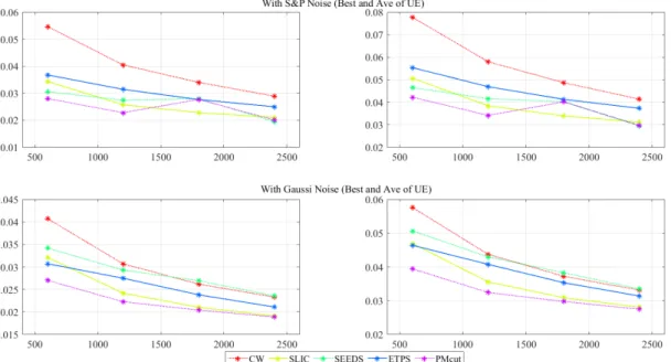
3.6 Undersegmentation error of each method. . . 41

3.7 Boundary recall of each method. . . 42

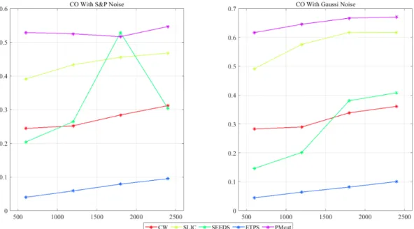
3.8 Compactness score of each method. . . 43

3.9 Superpixel results of5methods on images with Gaussian andS&P noise. 45 3.10 Comparing superpixel methods applied on Gaussian and denoised images. 46 3.11 Analysis of PMcut with differentσ and time limits. . . 47

4.1 The stair-casing effect of the total variation model. . . 50

4.2 A synthetic2D image with noise that has linear trend and its3D view. . 52

4.3 An example with3linear pieces and2active edges. . . 54

4.4 An example where an outlier exists. . . 55

4.5 An example where the optimal solution is not unique. . . 56

4.6 A counter-example where model (4.5) does not form a valid segmentation. 58 4.7 An example with a9-pixel segment. . . 59

4.8 A synthetic image with4affine pieces and with Gaussian noise, 2D and 3D view. . . 63

4.9 A synthetic image with4affine pieces plus background and with Gaus-sian noise, 2D and 3D view. . . 63

(12)

4.11 Segmentation results of MC-C. . . 67

4.12 Segmentation results of MC-B withξ3 = 3and1.5for the second image. 67 4.13 Segmentation results of MC (ξ2 = 0.5) and MC-M (ξ1 = 2.5) on the second image. . . 68

4.14 Segmentation results of MC-H. . . 69

4.15 Results of MC-M-B on the first image,2D and3D plot. . . 70

4.16 Output of TGV on the first image,2D and3D plot. . . 70

4.17 Results of MC-B-M on the first image,2D and3D plot. . . 71

4.18 Output of TGV on the second image,2D and3D plot. . . 71

4.19 Segmentation results of MC-B-M on two synthetic images. . . 71

4.20 Photo taken by a normal camera of HCIBOX (left) and inverse of the depth image (right). . . 72

4.21 3D plot of the HCIBOX instance. . . 72

4.22 Segmentation result of HCIBOX using MC-M-B. . . 73

4.23 The Teddy image (left) and the disparity map (right). . . 73

4.24 Left: segmentation result using our heuristic. Right: MC-M-B-C result. 74 4.25 Superpixel generation on the Teddy disparity map. . . 75

5.1 Two ways to provide user input for an interactive image segmentation . 77 5.2 TheK-nearest cut generation strategy . . . 86

5.3 Ground-truth generation on3images taken from the PASCAL dataset. . 89

5.4 Comparison of5proposed models on an MRI. . . 90

5.5 Comparison of4models plus ILP-PCW on an image from BSDS500. . 92

5.6 More experiments on4BSDS500 images. . . 93

5.7 Segmentation results with different user scribbles on the same image. . 96

(13)

List of Tables

3.1 Average time, optimality gap and energy of3proposed methods. . . 36

3.2 The combined OP score of5superpixel methods in one scenario. . . 43

3.3 Average OP score of5superpixel methods. . . 44

4.1 Statistics of MP with and without the4-edge cycle constraints. . . 66

4.2 Statistics of MC with and without the cardinality constraints (MC-C). . 66

4.3 Statistics of MC with and without the bounding constraints (MC-B). . . 67

4.4 Statistics of MC with different big M value. . . 68

4.5 Statistics of MC with and without the initial solution (MC-H). . . 69

5.1 Energy values of5proposed models. . . 91

(14)

List of Algorithms

2.1 Cutting plane method . . . 14

2.2 Branch-and-bound method . . . 15

3.1 `0 region fusion algorithm with`1 data term . . . 33

(15)

Chapter 1

Introduction

1.1

Motivation and Overview

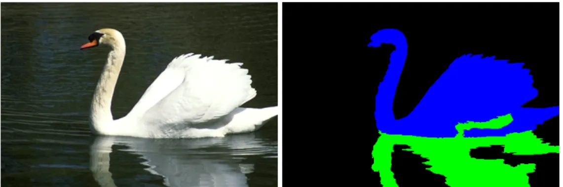
In computer vision, image segmentationis a fundamental task that partitions a digital image into multiple segments (set of pixels). The goal is to change the representation of an image from pixels into segments that are semantically more meaningful and easier to analyze. See Figure 1.1 for an example. More precisely, image segmentation is the problem of assigning labels (e.g., foreground and background labels) to all pixels in an image such that pixels with the same label share certain properties. It is typically applied to locate objects and boundaries within an image.

Figure 1.1 – Illustration of an image segmentation: left is the input image, right is a segmentation into meaningful segments.

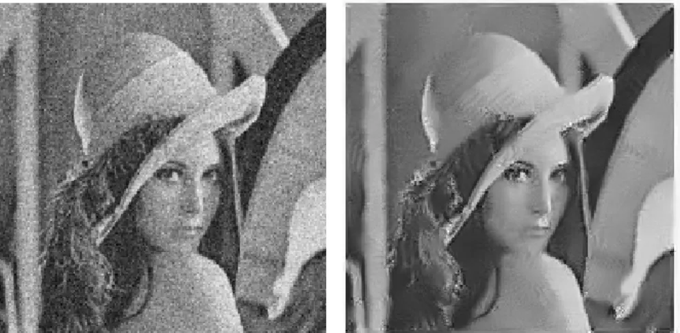
Image noiseis random variation of brightness or color in an image. The presence of noise in images is unavoidable, making it difficult to perform any required image processing tasks. Given a noisy image,image denoising is the operation of estimating the clean, original image. As can be seen in Figure 1.2, the right image becomes smooth, but on the downside, the sharp boundaries have also been smeared. Hence, the goal of any denoising algorithm is to remove the noise while still keeping the image sharp.

(16)

Figure 1.2 – Illustration of an image denoising: left is the input noisy image, right is the denoised image.

Usually, one first applies denoising method as a pre-processing step before segmen-tation. But as discussed above, the denoising algorithm may over-smoothen the sharp boundaries and hence harm the segmentation results.

In this thesis, we first combine these two problems into one framework, and propose a novel formulation for simultaneously denoising and segmenting a given noisy image. It is based on the well-known Potts model [1], and can be either a piecewise constant or affine model.

Secondly, we allow users to interact with the image, either to manually label some pixels, or to exclude the known outliers. We propose an interactive image segmentation approach, where the user is required to drawk scribbles, and the output is exactly k

connected segments. See Figure 1.3 as an example, where the input is the probability map trained with convolutional neural networks (CNN) of a magnetic resonance image (MRI), which depicts the abdominal aorta. The formulation is based on the Markov Random Field (MRF) model [2] and we introduce a global prior which enforces the connectivity of each label.

All the models in this thesis are formulated as Mixed Integer Linear Programs (MILPs). It is in generalN P-hard to solve a MILP, thus fast heuristic algorithms are usually beneficial in that they provide initial solutions to the MILP solver, as well as to the original problem. Sophisticated methods from combinatorial optimization such as branch-and-cut are implemented by default in any modern MILP solver, to get globally optimal solutions. The main advantage of our model over heuristics is that they pro-vide globally optimal solutions if no runtime restrictions are specified, hence propro-vides ground-truth results that could be used as quality assessment for any algorithms.

(17)

Figure 1.3 – Illustration of an interactive image segmentation: left is the input probabil-ity map with2user scribbles, right is the desired segmentation.

1.2

Contributions

The main contributions of this thesis are the following:

• We propose novel MILP formulations for both piecewise constant and affine Potts models.

• We explore facet-defining inequalities for the associated integer polytope of the piecewise constant Potts model.

• We conduct extensive benchmark comparison using several state-of-the-art super-pixel algorithms applied on noisy images.

• We explore additional constraints that enforce valid segmentation in the MILP formulation of piecewise affine Potts model.

• We revisit the Integer Linear Programming (ILP) formulation for multi-label MRF with connectivity priors and solve it to optimality.

1.3

Organization

This thesis is organized as follows: We start in Chapter 2 by giving basic definitions, starting from graph and polyhedral theory to mathematical programming, linear regres-sion, and finally to superpixels.

In Chapter 3, we first introduce the MILP formulation of the discrete piecewise constant (first derivative) Potts model and the multicut problem [3]. We prove that the multicut constraints are redundant for the the optimal solutions of the Potts model, but they are facet-defining for a special integer polytope. We also introduce a`1 norm fast heuristic based on the region fusion algorithm [4]. Due to the N P-hardness of the

(18)

corresponding optimization problem, we decompose the original image into rectangu-lar blocks (patches) and apply our model within each patch for generating superpixels on noisy images of the BSDS500 dataset [5] against other state-of-the-art superpixel algorithms.

Chapter 4 is devoted to the more general case where the input image is assumed to possess piecewise affine features. We propose a MILP formulation for the piecewise affine Potts model, and prove that the multicut constraints are needed to enforce a valid segmentation. We adapt the heuristic in [4] for the piecewise affine case which provides an initial solution to the MILP solver. Synthetic images as well as real depth images are tested to confirm the usefulness of our model.

In Chapter 5, we focus on the MRF model. We first revisit the ILP formulation of the pairwise MRF and introduce the concept of connected subgraphs. We then formulate the MRF with global connectivity as a MILP. For solution techniques, we again adapt the region fusion algorithm [4] to generate initial feasible solutions. We also discussion the strategy for selecting the cutting planes in the separation problem. Extensive com-putational experiments on standard image datasets as well as medical images are carried out using different variants of our proposed model.

Finally, we conclude this thesis and point out some future research directions in Chapter 6.

(19)

Chapter 2

Preliminaries and Terminologies

This chapter presents basic concepts needed throughout the thesis. Many of them are standard and can be found in the textbooks of the corresponding field, such as [6, 7]. We include them here to make the thesis more self-contained.

2.1

General Notation

Asetis a collection of distinct elements (also known as members). It is usually denoted by a capital letter, while vectors and scalars use small letters. A setB is called asubset ofA(denotedB ⊆A) if every member of B is also a member of A. IfB is a subset of

Abut not equal toB, thenB is aproper subsetofA(denotedB ⊂A). Thepower set ofA, denoted by_P(A), is the set of all subsets inA. Thecardinalityof a setA, denoted by|A|, is the number of elements ofA. Theunionof A and B, denoted byA∪B, is the set of all members of either A or B. Theintersectionof A and B, denoted byA∩B, is the set of all members of both A and B. TheMinkowski sumof two setsAandB is the set of all elementsx+ywithx ∈ A andy ∈ B. Apartitionof a setAis a collection of nonempty sets{A1, A2, . . . , An}, such that∪ki=1Ai = A, andAi ∩Aj = ∅, for any

i6=j.

We denote the set of real numbersR, the set of nonnegative real numbersR+, the set of natural numbers_N. We also denote[n]the set of integer numbers{1,2, . . . , n}.

Avectora∈_Rn×1_{is usually a column vector. The}_transpose_{of the column vector}_a_, denoted by a> ∈ _R1×n_{, is then a row vector. The} _{inner product} _{of two vectors} _a ₌

(a1, a2, . . . , an)> andb = (b1, b2, . . . , bn)> is denoted bya>b, and it equals Pn_i₌₁aibi.

The p-norm, also know as the `p norm of a vector a ∈ Rn, is denoted as kakp :=

(Pn

i=1|xi|p)

1/p

. In particular, the`1 normkak1 :=

Pn

i=1|xi|, and the`2 normkak2 :=

pPn

i=1x2i.In contrast, the`0 norm of a vectorais the number of nonzero entries. We denote a vector of all zeros of appropriate dimensions as0.

(20)

elements where operations like addition and multiplication are defined. Thetranspose of them×nmatrixDis denotedD> = (d0_ij)∈_Rn×m_where_d0

ij =dji.

For a logical expressionϑ, anindicator function₁(ϑ)is1ifϑis true and0otherwise.

2.2

Graph Theory

All the models in this thesis are defined on undirected graphs. We hence introduce concepts from graph theory that we will need later. The definitions are mostly taken from the fundamental part of [8], which is a good reference for further reading.

2.2.1

Undirected graphs

An undirected graph G = (V, E) (or simply G(V, E)) is a tuple of two basic finite setsV andEsuch thatE ⊆ V₂

. The elementsv ∈V are calledvertices(ornodes) and

e∈E called edges of the graphG. We denote the set of all nodes byV(G)and the set of all edges of a graphGbyE(G), respectively. We will denote an edgee={u, v} ∈E

simply byuv, so in an undirected graph,e = uv = vu. We call the nodes uandv the endnodesofe=uv. Two nodesuandvareadjacentifuv ∈E, and a nodeuisindident to an edge e, and vice versa, if u is an endnode of e. The neighborhood of a node u

is the setnb(u) := {v ∈ V | uv ∈ E}, and the degreeof node uis the cardinality of

nb(u). From now on, all the graphs discussed in this thesis are undirected graphs. A graph G0(V0, E0) is called a subgraph ofG(V, E) ifV0 ⊆ V andE0 ⊆ E. We also sayG0 is contained inGin this case.

2.2.2

Paths, cycles, and connectivity

In a graphG, apathbetween two nodesu1 anduk (which we call a(u1, uk)-path) is a

subgraphP(VP, EP)of G whereVP ={ui ∈V |i∈[k]}andEP ={uiui+1 ∈E |i∈

[k−1]}. Thelengthof a pathP is just|EP|.

A cycle is a subgraph C(VC, EC) of G where VC = {ui ∈ V | i ∈ [k]} and

EC = {uiui+1 ∈ E | i ∈ [k−1]} ∪ {uku1}. The lengthof a cycleC is just |EC|. If

there is a cycle C in G, then an edgee = uv ∈ E(G)is called a chord of C inG if

u, v ∈VC ande /∈EC. We call a cycleC ⊆Gchordlessif there is no chord ofCinG.

Two nodesu, v in a graphGareconnectedif there is a(u, v)-path inG. Gis called connectedif for any pair of nodes inG, there exists a path between them, otherwise it is disconnected. Aconnected componentof a graphGis a connected subgraph ofG, and is maximal with respect to edge inclusion.

(21)

2.2.3

Cuts and multicuts

For a graph G(V, E), the cut of G induced by a subset of nodes D ⊆ V is denoted

δ(D) := {uv ∈ E | u ∈ D, v ∈ V \D}. This definition is extended to disjoint sets

Di ⊂V, fori∈[n]andn ≥2, such thatδ(D1, D2, . . . , Dn) := {uv ∈E |u∈Di, v ∈

Dj, i 6= j, i, j ∈ [n]}. We call the set δ(D1, D2, . . . , Dn) a multicut of G induced

byD1, D2, . . . , Dn, ifD1, D2, . . . , Dnis a partition of V. The setsD1, D2, . . . , Dkare

called theshoresof the multicut.

2.2.4

Selected classes of graphs

Agrid graphof sizem×nis a graphG(V, E)such thatV ={(i, j)|i∈[m], j ∈[n]}

andE ={((i, j),(i+ 1, j))|i ∈[m−1], j ∈ [n]} ∪ {((i, j),(i, j+ 1)) |i∈ [m], j ∈

[n−1]}.

A weighted graphis a tupleG(V, E, w)whereG(V, E)is a graph and there exists an associatedweight functionw : E → _R(orw : V → _R) that assigns a weightw(e)

for each edge ofE(orw(v)for each node ofV).

2.3

Polyhedral Theory

The optimization models we formulate within this thesis will be mixed integer linear programs. However, the algorithms for solving such problems cannot be understood without some basic knowledge of polyhedral theory. We assume the readers are famil-iar with the standard linear theory such as the real vector space_Rm, subspaces, linear independence, scalar product, dimension and so on. The following notations and defi-nitions are mainly based on [7].

2.3.1

Convex and affine subspaces

Alinear subspaceof _Rm is a nonempty setD ⊆ Rm such that for allx1, x2 ∈ Dand

a1, a2 ∈ R, a1x1 +a2x2 is inD. Thus, a linear subspace always contain 0. An affine subspaceof_Rm _{is a subset} _A ₌ _x₊_D_{, where}_x _∈ _Rm _and_D_{is a linear subspace of}

Rm. Thedimensionof an affine subspace is the dimension of its associated linear vector space.

A linear combination of a set of vectors {x1, x2, . . . , xn} ⊆ Rm is defined by the

scalar product Pn

i=1aixi, where ai ∈ R is called the coefficient. It is called affine

combination if Pn

i=1ai = 1 and convex combination if in addition, ai ≥ 0, for i =

1,2, . . . , n. The vectors{x1, x2, . . . , xn}are calledaffinely independentif(xi−xn), for

(22)

A set S ⊆ _Rm _{is called} _convex _{if it contains all convex combinations of finitely}

many vectors inS. Theconvex hullof a setSis denoted by conv(S), and is the set of all convex combinations of vectors inS. Theaffine hullaff(S)is then defined analogously.

2.3.2

Polytopes and polyhedra

Anlinear inequality (constraint)a>x≤bdefines ahalfspace{x∈_Rn _|_a>_x_≤_b_}_and

a correspondinghyperplaneH(a, b) ={x∈_Rn_|_a>_x₌_b_}

.

ApolyhedraP can be defined as the intersection of finitely many halfspaces and is denotedP ={x∈ _Rn _|_Ax _≤ _b_}_{, where}_A _∈

Rm×n andb ∈ Rm. It is calledbounded if there exists a “box”Q = {x | l ≤ xi ≤ u,∀i ∈ [n]} ⊂ Rn with somelandu, such thatP ⊆ Q. A polytopeis a convex hull of a nonempty finite set, and it is a bounded polyhedra. It is clear that both the polyhedron and polytope are convex sets.

There are two ways to describe a polytope: the convex hull of a nonempty finite set, which is called V-representation, or the bounded intersection of finitely many closed half spaces, also calledH-representation.

2.3.3

Vertices, faces and facets

Consider a polytopeP ={x∈_Rn _|_Ax_≤_b_}_{. In order to find out the fewest necessary}

inequalities to describeP, we need the following definitions.

An equality a>x ≤ b is called avalid equality forP if it holds for allx ∈ P. Its corresponding halfspace and hyperplaneH(a, b)is calledsupportingifH∩P 6=∅. If in additionH 6=P, we call it aproper supporting hyperplane. The setF :=P ∩H(a, b)

is called thefaceof the polytopeP induced bya>x≤b. We callF aproper faceif the corresponding hyperplaneHis proper.

Thedimensionof a faceF (dim(F)) inP is the dimension of its affine hull aff(F). We call the face of dimension 0,1 and dim(P) −1 the vertex, edge and facet of P, respectively. A vetexvofP is often referred to as anextreme point.

An equality a>x ≤ b is calledfacet-defining if F = P ∩H(a, b)is a facet. The facet-defining inequalities are the most important ones to describe the polytope P. In fact, every polytope (fully-dimensional) is the intersection of the halfspaces defined by their facet-defining inequalities. One can show that this description is minimal with respect to the number of halfspaces.

2.4

Algorithms and Complexity Theory

Complexity theory investigates how difficult is the problem and the efficiency of the algorithms used to solve it. We briefly introduce the notations to these topics. For further information, [9] gives a good survey.

(23)

2.4.1

Algorithms, decision problems, complexity

Analgorithmcan be interpreted as a finite set of instructions on how to solve a problem, where each instruction contains a sequence of elementary steps on the input data, e.g., plus, minus, etc.

We introduce a functiontc : N →Rin order to measure the number of elementary

steps needed by an algorithm, and this function is called the time complexity of the algorithm, orcomplexityfor short. This function provides for each input of sizen ∈_N

the maximal elementary steps tc ∈ R. We denote an algorithm has a complexity of

O(g(n))if there exists two constantsc ∈ _R+_and _n

0 ∈ N, such thattc(n) ≤ c·g(n),

∀n ≥ n0. Ifg(n) is a polynomial function onn, then we saytc is a polynomial-time

algorithm. Or equivalently, the problem ispolynomial-time solvable.

Adecision problemcan be posed as a “yes” or “no” problem. Decision problems are mainly divided into two classes, namely classesP andN P. The set of all polynomial solvable decision problems is denoted by P. The class N P is defined as the set of all decision problems for which each input with an answer “yes” can be verified in polynomial time. Although it is clear thatP ⊆ N P, it is still an open question if the opposite holds. That is, we do not know ifP equalsN P or not.

Given two decision problemsDandD∗, Dis said to bepolynomial-time reducible toD∗ if there exists a polynomial algorithm that transforms each instance ofD toD∗

such that they always have the same answer. Informally, we say problemDis not harder than problemD∗.

A decision problemDis calledN P-complete if every problem inN Pcan be poly-nomial reducible toD. Informally speaking,N P-complete problems are the most dif-ficult problems in classN P.

2.4.2

Complexity of optimization problems

Anoptimization problem(or more precisely, a minimization problem) can be defined as the following:

min

x∈Xf(x)

where X is a set of feasible solutions to the problem, andf is a real-valued function onX.

We then assign the following decision problem to the optimization problem: “Given a constant c ∈ _R, is there an x ∈ X such that f(x) ≤ c”. This decision prob-lem is polynomial-time reducible to the optimization probprob-lem. Hence, the notion of polynomial-time reducible can also be applied to an optimization problem. We call an optimization problemOpt N P-hard if there exists anN P-complete decision problem that can be polynomial-time reducible toOpt. That is, if every decision problem inN P

(24)

When solving an optimization problem, anexact algorithmis one that always solves the problem to optimality when no time limit is constrained. On the contrast, aheuristic algorithmis one that not necessarily finds the optimal solution, or even if it finds the optimal one, there is no proof for that.

2.5

Mathematical Programming

In mathematics, computer science and operations research,mathematical programming (MP) ormathematical optimization, is to select a best element (with regard to a certain criterion) from a given set of available alternatives. We briefly review two special cases of MP, i.e., linear programming and mixed integer linear programming.

2.5.1

Linear programming

Linear Programming(LP) deals with obtaining the best outcome with respect to some requirements in forms of linear relationships. More formally, it has the following form:

min c>x

s.t. Ax≤b x∈_Rn_,

whereA ∈ _Rm×n _and _b _∈

Rm. Other forms of LP, such as maximization instead of minimization, great than equal to or equal restrictions, can be easily transformed to the above form.

The entries of the vectorx = (x1, x2, . . . , xn)are calledvariablesof the LP, them

conditionsAx ≤ b constraints, and the linear functionx → c>x objective functionof the LP. The setS := {x ∈ _Rn _| _Ax _≤ _b_} _{is called}_{feasible region, and its elements}

feasible solutionsof the LP. IfS 6=∅, the LP isfeasible. If an LP is feasible, a feasible solutionx∗ is called optimal solutionif and only ifc>x∗ ≤ c>x for any feasible solu-tionx. The corresponding valuec>x∗ is namedoptimal valueof the LP. Note that it is possible for more than one feasible solutionsx with c>x = c>x∗. If for any α ∈ _R, there exists a feasible solutionxsuch thatc>x≥α, then the LP is calledunbounded.

One key observation is that the feasible region of the LP is a polyhedra, and thus convex. If the LP has an optimal solution, this solution always occurs on the vertex.

There exists efficient algorithms for solving linear programming problems. Namely, thesimplex method, interior point method, andellipsoid method. The simplex method has exponential-time complexity in the worst case, while both the interior point and ellipsoid algorithm are polynomial-time solvable. But in practice, the simplex algorithm is found be remarkably efficient and the runtime is often polynomial. Hence, it is widely used to solve LPs.

(25)

Figure 2.1 – The feasible solutions is plotted in black dots, the integer hullPIis colored

in red, and is contained in the feasible regionP, which is colored pink.

2.5.2

Mixed integer linear programming

Amixed integer linear program(MILP) can be seen as an extension of a linear program, by exchanging some of its continuous variables to discrete ones. It has the following form:

min c>x+d>y (2.1)

s.t. Ax+By ≤e x∈_Rm_{, y} _∈

Zn,

where the requirementsy ∈_Zn_{are called the}_{integrality constraints. If there exist only}

discrete variables, it is called aninteger linear program(ILP). Ify∈ {0,1}n_{, we have a}

binary linear problem.

Acombinatorial optimization problem(COP) is to identify an optimal solution from a finite set of feasible solutions. It covers a wide range of practical problems. Most COPs can be formulated based on graphs, and then defined as MILPs.

Despite the similarity to the LPs, MILPs are much harder: general MILPs belong to the class ofN P-hard optimization problems.

For MILPs, the feasible region is naturally defined asP(A, B, e) :={x∈_Rm_{, y} _∈

Zn | Ax+By ≤ e}, and the LP relaxation of the feasible region as PL(A, B, e) :=

{x∈_Rm_{, y} _∈

Rn|Ax+By≤e}.

If P(A, B, e) is bounded, the feasible region of the MILP is finite. We define the integer hullPI(A, B, e)as

(26)

which is the convex hull of the feasible region. The associated polyhedraPI(A, B, e)satisfies

P(A, B, e)⊆PI(A, B, e)⊆PL(A, B, e),

with the inclusion being proper in general cases. One example is shown in Fig. 2.1, where we only have integer variables.

2.5.3

Solution methods for MILPs

The solution methods can be grouped into two types: exact and non-exact methods. Non-exact methods are usually heuristics or approximation methods. For any MILP, one can usually design a greedy or local search algorithm which can be used to compute an initial solution. Unfortunately, under the greedy mechanism, one can easily get trapped in a local minimal. An improved type of heuristic is calledmeta-heuristics, such astabu searchandsimulated annealing.

We will focus on two of the exact methods, namely, thecutting-plane method and thebranch-and-bound method. Before describing these two methods, we first introduce the notions of relaxation and separation problems.

A relaxationof an optimization problem minx∈Xf(x) is the optimization problem

minx∈X0f(x), whereX ⊆ X0. It immediately follows that ifx∗ is an optimal solution

of the original problem andx0 is an optimal solution of the relaxation, then

f(x0)≤f(x∗), (2.3)

i.e., solving the relaxed minimization problem yields a lower bound for the original one. The reason for considering the relaxation of the original problem is that the relaxed optimization problem may be easier to solve. For a MILP

min{c>x+d>y|Ax+By ≤e, x∈_Rm_{, y} _∈

Zn}

a natural relaxation is the so calledlinear programming relaxation(LP-relaxation) min{c>x+d>y|Ax+By≤e, x∈_Rm_{, y} _∈

Rn} which relaxes the integrality constraints ofytoy∈_Rn_.

We adopt the notationP(A, B, e), PI(A, B, e)andPL(A, B, e)from Section 2.1 to

denote the feasible set of the MILP, convex hull and LP-relaxation of the feasible set, respectively.

Aseparationproblem associated with a MILP min{c>x+d>y|x, y ∈P(A, B, e)}

is the problem: given(x0, y0)∈ _Rm×n_{, is}_(x0_{, y}0₎ _∈_P

I(A, B, e)? If note, the separation

problem finds a valid inequalityπ>x+ω>y ≤ π0 forPI(A, B, e), but violated by the

point(x0, y0). This inequality is then added to the problem that “cuts off” the current infeasible solution.

(27)

Cutting-plane method

We briefly describe the cutting-plane procedure: when solving a MILP, we first start with solving a relaxation of the problem. If the obtained solution (x0, y0)satisfies all the constraints of the MILP, it is then also the optimal solution of the original problem. However, this is usually not the case. The basic idea of a cutting-plane method is to come up with a separation problem with respect to the current solution and the original MILP. The valid inequality of this separation problem is called acutting planeor simply acut, since it “cuts” off (x0, y0)fromPI(A, B, e). We then add this valid inequality to

the current relaxation problem and this procedure is iterated, until the obtained solution satisfies all the constraints. This process is shown in detail in Algorithm 2.1.

The crucial point is how to solve the separation problem efficiently at each iteration, and if the cutting plane generated could cut off a large area of the relaxation polyhedra

PL(A, B, e). Ideally, good candidates for such cuts are those which define the facets

ofPI(A, B, e). However, one needs to balance the efficiency of finding a cut, and the

quality of the cut. Another thing to note is that it may not be useful to add many facet-defining inequalities all at once, but only to add those that cut off the current solution of the relaxation problem. Finally, it is not practical to stop the loop of separation problem until no violated cuts can be found. For instance, one could stop once the solution of the relaxation has improved, which could still be useful to the branch-and-bound method to be discussed in the next section.

There exists different ways of generating the cutting planes, and the first cutting plane procedure was developed in the 1950s by Gomory [10]. Gomory was able to specify an easy way to generate such cuts that guarantees to find an feasible solution to

PI(A, B, e)within a finite number of iterations.

Branch-and-bound method

Branch-and-bound method is a general approach for solving MILPs. It is based on the following two conclusions:

• Consider the objective value z = minx,y {c>x +d>y | (x, y) ∈ P(A, B, e)},

let P = P1 ∪P2. . .∪PK be a decomposition of P into subsests, and let zk =

minx,y {c>x+d>y|(x, y)∈Pk}fork = 1,2. . . , K. Thenz =minkzk.

• Let zk _{be a lower bound on} _zk_{, and} _z_¯k _{an upper bound on} _zk_{. Further let} _z ₌

minkzkandz¯=minkz¯k. Thenz is a lower bound andz¯an upper bound onz.

As the name suggests, it consists of two main steps: branching and bounding. The key idea behind this algorithm is to split the original hard problem into easier smaller problems, calledsubproblems. The subproblems can be solved, fathomed or split into subproblems again. This leads to the constriction of a branch-and-bound tree with the

(28)

Algorithm 2.1Cutting plane method

1: Initialize:t ←0, P0 ←PL(A, b, e).

2: while (stopping criterion not reached)do

3: Solve the LP(xt_{, y}t_{) =}_argmin x,y{c >_x₊_d>_y_|_{(x, y)}_∈_Pt_}_. 4: ifyt∈_Zn_then 5: (xt, yt)is an optimal solution. 6: break 7: else

8: Solve the separation problem with respect to(xt_{, y}t₎_and_P

I(A, B, e).

9: if∃a valid inequalityπt>_x₊_ωt>_y_≤_πt

0 that cuts off(xt, yt)then

10: Pt+1 ←Pt∩ {πt>x+ωt>y≤π₀t}. 11: t←t+ 1. 12: else 13: break 14: end if 15: end if 16: end while

LP relaxation of the MILP as the root node. In addition, we keep track of the global lower and upper bound, which helps to fathom some branches of the tree and also pro-vides a relative gap called theoptimality gap. In a minimization problem, It is computed as follows:

optimality gap= |z¯−z| ¯

z .

The method terminates if there is no more subproblems to be solved, or if the opti-mality gap is relativity small. The advantage of this method is that the basic principle is simple, and it can be adopted to solve any MILP. Moreover, one can use any heuristic or approximation algorithm to compute an initial solution as an upper bound.

We can then solve the MILP in the following way. First, we solve the LP-relaxation of the MILP, which serves as the root node of the branch-and-bound tree. If the result-ing solution satisfies all the integrality constraints, we have already solved the original problem. If not, we select variableyi for somei∈ [n]which has fractional value y∗ in

the LP solution. We then split the current problem into two LP subproblems, one with constraintyi ≤ by∗ic, and the other with constraintyi ≥ dyi∗eadded. We then execute

the same procedure of splitting current node into two new LP subproblems, if the re-sulting solution is not feasible to the original MILP. Meanwhile, if a subproblem gets a feasible solution, we update the global upper boundz¯. If it has fractional solution, we fathom the current node and update the global lower boundz. The process stops when there exists no unsolved subproblems, or ifz¯=. z. Denote the set of all subproblemsP,

(29)

the details of this algorithm can be seen in Algorithm 2.2.

Algorithm 2.2Branch-and-bound method

1: Initialize:z ← −∞,z¯←+∞,P ←PL(A, b, e).

2: while P 6=∅do

3: Choose a subproblem P ∈ P and solve the LP-relaxation. Denote the optimal solution and objective value as (x∗, y∗) and z∗, if they exist.

{Subproblem selection}

4: ifP is infeasible orz∗ ≥z¯then

5: FathomP. {Fathoming}

6: else ify∗ ∈_Znandz∗ <z¯then

7: z¯←z∗. {Bounding}

9: else

10: Select one fractional variable yi and add two new subproblems: P ∩ {yi ≤

by_i∗c}andP ∩ {yi ≥ dyi∗e}toP. {Branching}

12: Computez∗ =minkzkfor the LP-relaxation of both subproblems.

13: ifz∗ > zthen

14: z ←z∗. {Bounding}

15: end if

16: end if

17: end while

The critical issue in Algorithm 2.2 is how to select the next subproblem in Step 3 and how to split the current node in Step 10. Different problem selection and branching strategies will lead to various branch-and-bound trees, thus different solution time. The recent paper [11] adopts supervised machine learning approach to learn how to branch from previous experiences, and it outperforms existing heuristic based branching strate-gies on benchmark instances.

Branch-and-cut method

Branch-and-cut is a technique that combines the branch-and-bound with the cutting plane method. It is the building block of many modern MILP solvers, hence is of great practical importance.

We will only state the basic idea of this method as follows: First, we compute the LP-relaxation of the MILP. Different from the pure branch-and-bound method, before branching, we first successively add violated inequalities (cutting planes) to strengthen the LP relaxation (cutting phase). This phase is stopped when no cuts can be found or a user-set time limit is hit. Then we begin with the branching phase that works as

(30)

in Algorithm 2.2 and we obtain two new subproblems. The above procedure is then applied to the next subproblem until no subproblem exists or if the optimality gap is almost0.

2.6

Constant and Affine Regression

Givennsignalsp = (p1, p2, . . . , pn)in ad-dimensional space, we denote their

coordi-natesz = (z1, . . . , zn)T ∈ _Rn×d _{and intensities}_y _{= (y}

1, . . . , yn) ∈ Rn. In this thesis,

we are interested in the casesd∈ {1,2}, and signalspcorresponding to pixels in a reg-ular grid whend= 2. In this case,yidenotes the RGB color grayscale value of pixelpi.

For computational efficiency, we restrict ourselves to the grayscale image in this thesis.

2.6.1

Parametric affine regression

In statistics,affine (linear) regressionorlinear fittingis a widely used approach to model the relationship between the dependent variablesyand independent variablesz. In the parametric model, the relationship is modeled using linear functions and the unknown linear parameters (i.e., slopes and intercepts) β are estimated from the given data ac-cording to some objective functions, such as the mean square error (MSE) [12]. It is also calledlinear least squares.

For instance, whend = 1, if we denote the fitting value of signalpi aswi, then the

mean square errorS =Pn

i=1(yi−wi)2. Herewi =β1∗zi+β0 andβ = (β1, β0)is the linear parameter of the fitting line, whereβ1 ∈Rdis the slope (gradient) andβ0 ∈Rthe intercept. The only two variables here areβ1 andβ0. So, the following minimization problem min β1,β0 n X i=1 (β1 ∗zi+β0−yi)2 (2.4)

is an unconstrained quadratic programming problem. We can get the analytical solution by setting its gradient to zero. The partial derivatives of MSE with respect toβ1andβ0 are: ∂S ∂β1 = 0 = 2 n X i=1 zi (β1∗zi+β0−yi), ∂S ∂β0 = 0 = 2 n X i=1 (β1∗zi+β0−yi).

This results in a system of two equations with two unknowns, which can be easily solved. Whenβ1 = 0, it becomes a constant fitting problem.

(31)

In general, let 1 = (1,1, . . . ,1) ∈ _Rn _and_Z _{= [Z}0 ₁_] _∈

Rn×(d+1), whereZ0 =

(z1, z2. . . , zn)T ∈ Rn×d. The affine least squares is to find the optimalβ = (β1, β0)∈ Rd+1that has the least mean square error of the following overdetermined system:

(Z>Z)β =Z>y.

Finally,β is the coefficient vector of the least-squares hyperplane, expressed as

β = (Z>Z)−1 Z>y.

2.6.2

Nonparametric affine regression

Non-parametricaffine (linear) models computewwithout explicitly modeling the affine parametersβ as variables. Letw = (w1, . . . , wn) ∈ Rnbe the fitting values (unknown

variables) of the input signals, the non-parametric linear least squares problem becomes

min n X i=1 (wi−yi)2 (2.5) wi−2wi+1+wi+2 = 0, i∈[n], (2.5a) wi ∈R, i∈[n−2], (2.5b)

where (2.5a ) implicitly enforces all fitting values lie in the same linear function with respect to the coordinates (to be discussed with more details in Chapter 4). If it is a constant fitting problem, we just need to replace (2.5a ) with the equality constraints

wi−wi+1 = 0, for alli∈[n−1].

Note that we could use any norm other than the`2 norm. In this thesis, we will use the`1as our data term. We will explain this in more details in the next chapter.

2.7

Decomposition via Superpixels

Nowadays, typical sizes of images easily exceed millions of pixels. In this thesis, we are mostly dealing with MILPs, which means the number of integer variables could be millions if we deal with original images. Hence efficient decomposition methods are crucial to us.

On the one hand, one can use typical integer programming decomposition tech-niques, such as cutting planes and column generation [13] method, which decompose a large problem into simpler ones while still being equivalent to the original. In addition, they can be applied to any general MILP.

On the other hand, since the main application in this thesis is image processing, we will introduce a decomposition technique that is solely developed for this task. This

(32)

reduction is implemented on the input data, in particular, a grid of pixels of the image. This preprocessing cannot be reversed in the optimization step of the reduced model, implying that it is not an equivalent reformulation: an optimal solution of the decom-posed model is not necessarily an optimal solution of the original one, thus a trade off between complexity and accuracy.

2.7.1

Superpixels

While the exact definition is vague, asuperpixelis regarded as a group of perceptually meaningful connected blocks of an image. A superpixel should contain pixels similar in color or other properties, which are likely to belong to the same physical world ob-ject. The concept of superpixels was introduced by [14], and was motivated by two aspects: firstly, a grid of pixels is not a natural representation of real world scenes, but just a digital imaging “artifact”; and secondly, the huge number of pixels in natural im-ages prevents many computer vision algorithms being computationally efficient or even possible.

Superpixels are usually used as a pre-processing step to speed up computations. Computational efficiency comes from the reduction in the number of elements of a given image, with the superpixel then being treated as a single variable. Superpixels thus have been actively applied for a wide range of applications, and there exist many contributions, see [15, 16] for an overview. Superpixels can be naturally obtained as the results of some image segmentation algorithms. To decrease the risk of the superpixels crossing object boundaries, these algorithms are applied in an over-segmentation mode. Examples are graph based[17], and normalized cuts[18].

Ideally, the following properties are desired for any superpixel algorithms, i.e., su-perpixels (or superpixel algorithms) should

• adhere well to image boundaries,

• be regular in shape and size, with smooth boundaries, • be able to control its number and size,

• be non-overlapping and thus each pixel is assigned a label, • represent connected sets of pixels,

• have few parameters, so that it can be easily adjusted, • be fast to generate.

There are advantages of superpixels with regular shapes and sizes. Apart from visual appealing, in case a superpixel does cross the boundary, since the size is controlled, the error rate as well.

(33)

Figure 2.2 – Illustration of the “leakage” of superpixels, which is measured by the un-dersegmentation error. The ground-truth segment is with the black border, and the red lines are superpixel boundaries. In this example, the areas shaded pink count towards the undersegmentation error.

2.7.2

Evaluation metrics for superpixels

Apart from being visually appealing, there are some quantitative measurements to eval-uate different superpixel algorithms. Given ground-truth image segmentations (usually annotated by a human), we will introduce and use three of them in this thesis, namely, the undersegmentation error, boundary recall, and compactness score. Of course, these are not the only evaluation metrics in the literature. For more details on evaluating superpixel algorithms, we refer the reader to a recent survey paper [16].

Undersegmentation Error

The undersegmentation error (UE) measures the amount of “leakage” of superpixels when placed over ground-truth segments, which also implicitly measures boundary ad-herence. Given ground-truth segments G1, G2, . . . , GM and superpixels of any

algo-rithmS1, S2, . . . , SL, the undersegmentation error UE is defined as

UE(G, S) := 1 N   X Gi X Sj∩Gi6=∅ min {|Sj ∩Gi|,|Sj −Gi|}  , (2.6)

where N is the number of pixels of the image. Overall, lower UE is preferred. This is illustrated in Figure 2.2.

Boundary Recall

Theboundary recall(Rec) is the most commonly used metric to measure the boundary adherence of the superpixel to the ground-truth segmentation. It computes the fraction of pixels on the boundary of ground-truth segments that lies within a small distance oft

(34)

Figure 2.3 – Illustration of the boundary recall: The boundary of a ground-truth segment (black) counts towards the boundary recall (without the dotted black lines) if it is within a distance of t to the boundary of a superpixel (pink).

Rec(G, S) :=

P

p1[p∈∂Gi for some i]·1[d(p, ∂Sj)≤t for some j]

P

p1[p∈∂Gi for some i]

, (2.7)

where ∂Gi and ∂Sj denote the border of the segments, d is the minimal distance of

a pixel p to the border of a segment, and t is a user-defined threshold. In this thesis, we will follow the convention in the paper [16] and let t = 3. See Figure 2.3 for an example.

Compactness Score

The compactness score (CO) compares the area A(si) of each superpixel si with the

area of a circle with the same perimeterP(si) of the superpixel. The later forms the

most compact2-dimensional shape, and a higher CO is usually desired. It is invariant to the ground-truth segmentations. CO is computed as

CO(G, S) = 1 N X Si |Si| 4πA(Si) P(Si) . (2.8)

(35)

Chapter 3

Piecewise Constant Potts Model for

Segmentation and Denoising

Image segmentation and denoising are two fundamental tasks in computer vision and image processing. Graph based models are popular for segmentation and variational models are employed for denoising. Our approach could address both problems at the same time. In this chapter, we propose a novel Mixed Integer Linear Programming (MILP) formulation of the discrete first derivative (piecewise constant) Potts model with `1 data term, where binary variables are introduced to deal with the `0 norm of the regularization term. We utilize the branch-and-cut method for global optimum, as well as a fast heuristic algorithm for approximate solutions that is based on the region fusion algorithm [4]. The MILP is solved by a standard off-the-shelf MILP solver, i.e., Cplex [19]. Computational experiments are conducted against the multicut prob-lem and using different variants of our proposed model. We also apply our method to generate superpixels on noisy images. Extensive experiments are carried out on the BSDS500 [20] image dataset and compared with other superpixel methods. Our method achieves the state-of-the-art in terms of a combined score (OP) composed of the under-segmentation error, boundary recall and compactness.

3.1

Background

The image segmentation problem, also known as partitioning, grouping, or clustering, is a fundamental problem in image processing. It contains the task of dividing an image into either fixed or unfixed number of non-overlapping regions. Problem representations are usually based on a graphG= (V, E), where nodesV relate to pixels or superpixels in an image, and E represents the set of edges consisting of unordered pairs of nodes indicating adjacency relations. A segmentation problem can be represented either by

(36)

Figure 3.1 – Two representations of an image segmentation: node labeling (by their colors) and edge labeling via multicuts (dashed edges).

• edge labeling: a multicut defined by a subset of edgesE0 ⊆E, which also results in a partition of a set of nodes, as can be seen in Figure 3.1.

We assume that the input is an image with pixels located on a grid. An image segmentation is then a partition ofV into sets{V1, V2, . . . , Vk}such that∪ki=1Vi = V,

andVi∩Vj =∅,i6=j. So in graph-theoretical terms, the problem of image segmentation

corresponds to graph partitioning.

One often distinguishes betweensupervisedandunsupervisedsegmentation. In the former case, the number of classes (e.g., person, grass, sky, etc) defined by labels is pre-defined, together with a function (often called the unary data term) measuring how likely a node belongs to each class. Among many existing supervised models, the Markov Random Field (MRF) is well studied and applied, interested readers may re-fer to [21, 22, 2] for an overview of this field. In the latter unsupervised case, such class information is missing. This introduces ambiguities when node labeling is used. Think about the node labeling in Figure 3.1, if we permute the labels (colors), it will result in the same segmentation. However, edge labeling (e.g., by multicuts) does not exhibit such symmetries and is therefore more appealing in the unsupervised case.

In this chapter, we focus on the problem of partitioning a given image into an un-known number of segments using edge labeling. Exact optimization algorithms such as themulticut problem[3, 23] and thelifted multicut problem[24] with positive or nega-tive edge weights are based on the Integer Linear Programming (ILP) formulation. They are in generalN P-hard, and globally optimal solutions can be solved iteratively using branch-and-cut methods. More efficient fusion move algorithm are adopted in [25, 26]. Denoising of images is one of the most basic image restoration problems. While some denoising approaches [27, 28] either estimate every pixel separately by fusing other “similar” neighboring pixels, or denoise several similar patches simultaneously. Global models like the total variation model [29] by Rudin, Osher, and Fatemi is one of

(37)

the best known variational denoising model. LetD∈_Rd_{denote the signal domain, and}

y : D → _Rdenote the given signals’ intensity values possibly with noise. Total vari-ation [29] basically approximates the input signalsywith a piecewise smooth function

w:D→_R, and is stated as min w Z D (w(z)−y(z))2dz+λ Z D |∇1w|dz. (3.1)

Here,z denotes the coordinate system of the signals (horizontal and vertical-axis if the input is a2D image), and the first part represents the data fidelity term (how wellwfits

y), while the second is the regularization term, withλ >0the user defined penalty term. Recall that ∇1 _{= (∂}

z1, ∂z2)represent the differential operation of the first order in the

2D case.

With (3.1) being convex, it can be efficiently solved with structured convex solvers. However, the`1 regularization term sometimes over-penalizes the sharp discontinuities between two distinct regions in an image. In these cases, denoising approach with Potts priors [1] is designed to preserve the sharp discontinuities while removing noises and thus more desirable.

Given two nodes p, q ∈ V, their continuous valuesw(p), w(q) and a constant λpq

that depends onp, q, thePotts function

θpq(w(p), w(q)) = λpq·1(w(p)6=w(q))

is discontinuity-preserving and widely used in computer vision. Recall that₁(·)is1if its argument is true and0otherwise.

We are most interested in the discrete setting of the Potts model [1]. Given n sig-nals [n] (recall that [n] denotes the discrete set {1,2, . . . , n}), the classical (discrete) piecewise constant Potts model (named after R. Potts) has the form

min

w kw−ykk+λk∇

1

wk0, (3.2)

wherew, ydenotes thenarray vector, the data term measures their`knorm difference,

and the regularization term measures the number of oscillations in w. Recall that the discrete first derivative ∇1_w _{of a vector}_w _∈

Rn is defined as then−1 dimensional vector(w2−w1, w3−w2, . . . , wn−wn−1)and the`0norm of a vector is its number of nonzero entries. Various modifications and improvements have been made for the Potts model, see [30] for an overview.

In general, solving the discrete version of the Potts model (3.2) is also N P-hard. Approximate algorithms such as local greedy methods [4] and alternating direction method of multipliers (ADMM) [31] are used instead. Recently, [32] utilizes a MILP formulation to deal with a similar problem in statistics called thebest subset selection problem. These papers all use the `2 data term, i.e., k = 2. In 1D, the Potts model

(38)

with`1 data term can be efficiently solved by dynamic programming. AnO(n2logn) algorithm is given in [33], anO(n2)algorithm in [34], and anO(nk)algorithm in [35], wherenis the number of input signals, andk ≤nis the number of unique values in the signals.

Motivated by the discrete Potts (3.2) and the work of [31], we will look into the prob-lem of simultaneously segmenting and denoising images. However, different from [4, 31] where`2norm is used and only approximate solutions are solved, we focus on the`1 data term and the exact algorithms which leads to globally optimal solutions of (3.2). This is possible in terms of a MILP formulation which isN P-hard. Hence we further introduce a fast region fusion [4] based heuristic with`1data term.

Highlights of this chapter.

• We propose a MILP formulation for the discrete Potts model (3.2) with `1 data term, which solves it to global optimum.

• We prove the multicut constraints [3] are redundant for the optimal solutions of MILP formulation, but also facet-defining for the associated integer polytope. • We propose a fast region fusion based heuristic algorithm for solving the Potts

model with`1data term.

• We apply our proposed method for generating superpixels on noisy images, and achieve state-of-the-art results on the proposed OP score.

3.2

MILP Formulation of the Piecewise Constant Potts

Model

Given n signals [n] in some interval D ⊆ _Rd _{with intensities} _y _{= (y}

1, . . . , yn). We

are most interested in the case whend = 2, where signals become image pixels andy

represent pixels’ color or gray-scaled values.

We call a functionf piecewise constant overDif there exists a partition of Dinto subintervalsD1, . . . , Dk such thatD= ∪ki=1Di, whereDi∩Dj =∅, andf is constant

when restricted to each Di, fori ∈ [k]. Throughout this chapter, we assume the input

signals or images contain noises. We treat the task of segmentation and denoising input signals as a piecewise constant fitting problem. We denote the fitting value for signali

aswi =f(i).

3.2.1

Formulation of 1D signals

For the 1D signals case, the associated graphG(V, E)simply becomes a chain graph, whereV ={i|i∈[n]}andE ={e = (i, i+ 1)| i∈[n−1]}. Denote two end nodes

(39)

Figure 3.2 – 1D piecewise constant fitting, with 3 segments and 2 active edges.

of an edgeeasheandte. We would like to formulate the Potts model (3.2) as a MILP,

this is achieved by introducingn−1binary variables

xe =

(

1, ifhe, teare in different segments

0, otherwise, and the following properties should hold

∇1_w

e= 0 ⇔xe= 0, ∀e∈E, (3.3)

∇1

we6= 0 ⇔xe= 1, ∀e∈E. (3.4)

Here, ∇1_w

e := whe − wte. The edge e is called an active or jump edge if xe = 1,

otherwise it is dormant. Upon the above assumptions, the fitting values w satisfy the piecewise constant property that we desire, i.e., the signals between two active edges define one segment whose fitting values wshare the same intensity and the number of segments equal P

e∈Exe + 1. See Figure. 3.2 for one example, where there are two

active edges and three segments.

The properties (3.3, 3.4) can be modeled via Mixed Integer Programming (MILP) using the “bigM” technique, which leads to the following formulation:

min X i∈V |wi−yi|+λ X e∈E xe (3.5) |∇1_w e| ≤M xe, ∀e∈E, (3.5a) wi ∈R, ∀i∈V, (3.5b) xe ∈ {0,1}, ∀e∈E, (3.5c)

where the first part of the objective function is the data fitting term, and the second is the regularization term. To prevent the model from over-fitting, a user defined parameter

(40)

λ > 0 is introduced to indirectly control the number of segments. The constant M

in (3.5a) is usually called a ”big M” constant, and it should be large enough so that (3.5a) is always valid when∇1_w

e 6= 0.

Lemma 3.1. The optimal solutions (w?_{, x}?₎ _{of problem} _(3.5) _{satisfy properties 3.3}

and 3.4.

Proof. Letϑ = P

i∈V |wi −yi|+λ

P

e∈Exe be the objective value of problem (3.5),

we proof sufficient and necessary conditions of 3.3 and 3.4. 1. ∇1_w

e = 0 ⇒ xe = 0.If ∇1we = 0, by constraint (3.5a), xe can be either 0or

1. But the optimality of the solution will enforce xe = 0since problem (3.5) is a

minimization problem andλ >0, and this makesϑsmaller.

2. xe = 0⇒ ∇1we = 0.Ifxe = 0, then it immediately follows by constraint (3.5a)

that∇1_w

e≤0, and hence∇1we = 0.

3. ∇1_w

e 6= 0 ⇒ xe = 1. If∇1we 6= 0, it immediately follows by constraint (3.5a)

thatxe = 1, whereM is assumed to be big enough for (3.5a) to hold.

4. xe = 1 ⇒ ∇1we 6= 0. Ifxe = 1, suppose we have∇1we = 0, then by part 1 of

this lemma,xe= 0, thus a contradiction.

Now we have proved that the optimal solution to (3.5) satisfies the piecewise con-stant property that we desire. Note that we use the`1 norm because it is more robust to outliers than `2 [36]. Moreover, it can be easily modeled with linear constraints. Namely, constraint (3.5a) is firstly replaced by the two constraints∇1_w

e ≤ M xe and

−∇1_w

e ≤ M xe. Secondly, the term |wi−yi|is replaced byε+i +ε

−

i wherewi−yi =

ε+_i −ε−_i andε+_i , ε−_i ≥0.

Problem (3.5) is then formulated as the following MILP

min X i∈V (ε+_i +ε−_i ) +λX e∈E xe (3.6) ∇1_w e≤M xe, ∀e ∈E, (3.6a) −∇1_w e≤M xe, ∀e ∈E, (3.6b) wi−yi =ε+i −ε − i , i∈V, (3.6c) ε+_i , ε−_i ∈_R+, ∀i∈V, (3.6d) wi ∈R, ∀i∈V, xe∈ {0,1}, ∀e ∈E.

(41)

Lemma 3.2. The MILP formulation(3.6)is equivalent to(3.5)

Proof. The equivalence of constraint (3.5a) with constraints (3.6a, 3.6b) is quite obvi-ous. Here, we concentrate on proving the second replacement.

Suppose wi ≥ yi, letwi −yi = c wherec is a constant, so we have |wi −yi| =

wi −yi = c. By constraint (3.6c), ε+i −ε − i = wi −yi = c. Then ε+i = ε − i +c, and ε+_i +ε−_i = 2ε−_i +c.

Since problem (3.5) is a minimization problem and by constraint (3.6d), the optimal solution will haveε−_i = 0andε+_i =c. Hence,ε+_i +ε−_i =c= |wi −yi|, which makes

the objective function of problem (3.6) and (3.5) the same.

The case whenwi ≤yican be proved similarly, and we omit the proof here.

Note that this technique of equivalently transforming (3.5) to (3.6) will be used widely in this thesis, and from now on, we will just specify the MIP formulation in the form of (3.5).

The optimal solution of (3.6) gives the fitting valuewifor the node (signal)iand the

boundaries of two segments (when xe = 1). The segmentation is uniquely defined by

the optimal solutionx, and we obtained denoised signals with valuewsimultaneously.

3.2.2

Formulation of 2D images

Given a 2D gray-scaled image, following notations from the previous section, the as-sociated graphG(V, E)is a grid graph. The first derivative Potts model in 2D is again modeled as a MIP, and could be formulated using exactly the same notation as (3.5). However, we propose to formulate it a bit differently as we will need it for introducing the cardinality constraints in Section (3.3.3).

SinceGis a grid graph, we divideEinto its row (horizontal) edge setEr_{and column}

(vertical) edge set Ecso that E = Er∪Ec andEr∩Ec = ∅. Suppose the input2D image is of sizem×n. We further denoteEr₌_{_Er

1, E2r, . . . , Emr}, whereEiris the set

of row edges in thei-th row andi∈[m]. Similarly, we haveEc₌_{_Ec

1, E2c, . . . , Enr