A Scalar Projection and Angle based Evolutionary
Algorithm for Many-objective Optimization
Problems
Yuren Zhou, Yi Xiang, Zefeng Chen, Jun He and Jiahai Wang,
Member, IEEE
,
Abstract—In decomposition-based multi-objective evolutionary algorithms, the setting of search directions (or weight vectors), and the choice of reference points (i.e., the ideal point or the nadir point) in scalarizing functions, are of great importance to the performance of the algorithms. This paper proposes a new decomposition-based many-objective optimizer by simultaneously using adaptive search directions and two reference points. For each parent, binary search directions are constructed by using its objective vector and the above two reference points. Each individual is simultaneously evaluated on two fitness functions— which are motivated by scalar projections—that are deduced to be the differences between two penalty-based boundary intersection (PBI) functions, and two inverted PBI functions, respectively. Solutions with the best value on each fitness function are emphasized. Moreover, an angle-based elimination procedure is adopted to select diversified solutions for the next generation. The use of adaptive search directions aims at effectively handling problems with irregular Pareto-optimal fronts, and the philoso-phy of using the ideal and nadir points simultaneously is to take advantages of the complementary effects of the two points when handling problems with either concave or convex fronts. The performance of the proposed approach is compared with seven state-of-the-art multi-/many-objective evolutionary algorithms on 32 test problems with up to 15 objectives. It is shown by the experimental results that the proposed algorithm is flexible when handling problems with different types of Pareto-optimal fronts, obtaining promising results regarding both the quality of the returned solution set and the efficiency of the new algorithm.
Index Terms—Many-objective optimization; evolutionary algo-rithms; dynamic decomposition; reference points
Manuscript received August xx, 2016; revised xxx xx, 2016, and xxx xx, 2016; accepted xxx xx, 2017. Date of publication xxx x, 2017; date of current version xxx xx, 2017. This paper was supported in part by the National Natural Science Foundation of China under Grants 61773410, 61673403, U1611262 and 61472143; in part by the Foundation of Key Laboratory of Machine Intelligence and Advanced Computing of the Ministry of Education under Grant MSC-201602A; in part by the Scientific Research Special Plan of Guangzhou Science and Technology Programme under Grant 201607010045; and in part by the Excellent Graduate Student Innovation Program from the Collaborative Innovation Center of High Performance Computing.
Yuren Zhou, Yi Xiang, Zefeng Chen and Jiahai Wang are with the School of Data and Computer Science, Sun Yat-sen University, Guangzhou, P. R. China. (E-mail: [email protected] (Y. Zhou), gzhuxiang [email protected] (Y. Xiang), [email protected] (J. Wang) and [email protected] (J. He)). Yuren Zhou is also with the Key Laboratory of Machine Intelligence and Advanced Computing (Sun Yat-sen University), Ministry of Education, P. R. China.
Yuren Zhou and Yi Xiang are also with the Collaborative Innovation Center of High Performance Computing, Sun Yat-sen University, Guangzhou, P. R. China.
Jun He is with the School of Science and Technology, Nottingham Trent University, Nottingham NG11 8NS, U.K.
Color versions of one or more of the figures in this paper are available online at http://ieeexplore.ieee.org.
Digital Object Identifier xxxxxxxxxxxx
I. INTRODUCTION
M
ULTI-objective optimization problems (MOPs) with at least four conflicting objectives are known as many-objective optimization problems (MaOPs) [1], [2]. Due to extensive existences of MaOPs in real-world applications, such as automotive engine calibration [3], water resource system planning [4], car controller optimization [5] and optimal product selection from software product lines [6], they have recently drawn steady attention in the evolutionary multi-objective optimization (EMO) community. A number of many-objective evolutionary algorithms (MaOEAs) have been spe-cially designed to handle MaOPs [7]–[15]In this paper, the following unconstrained MOP (or MaOP) is considered.
Minimize F(x) = (f1(x), f2(x), . . . , fm(x))T,
subject to: x∈Ω, (1)
where x = (x1, x2, . . . , xn)T is the decision vector, and
n denotes the number of decision variables. In MOP (1),
Ω ⊆Rn is called the decision space; F(x) ∈ Rm, denoting the objective vector of x, consists of m objective functions fi(x), i= 1,2, . . . , m. Due to the nature of conflict among all the objectives, there is no single optimal solution available for an MOP, but a set of solutions representing trade-offs among different objectives. For solutionsxandy,xis said to Pareto dominateyif and only iffi(x)≤fi(y)holds for every
1 ≤ i ≤ m and there exists at least one j ∈ {1,2, . . . , m} such thatfj(x)< fj(y). If neitherxPareto dominatesynory Pareto dominatesx, then they are Pareto non-dominated with each other. A solutionx∗ is Pareto-optimal if there is no other solution x ∈Ω such that x Pareto dominates x∗. The F(x∗)
is then called the Pareto-optimal (objective) vector. All the Pareto-optimal solutions constitute the Pareto-optimal set (PS). Accordingly, the set of all the Pareto-optimal vectors is called the Pareto-optimal front (PF) [9].
Being simple, flexible, free from derivatives and being able to approximate the true PF with multiple solutions in a single run [16], [17], multi-objective evolutionary algorithms (MOEAs) have achieved great successes when optimizing MOPs with mostly two or three objectives [18]–[22]. Since the output of MOEAs for an MOP is a set of Pareto non-dominated solutions, Pareto dominance naturally becomes a feasible criterion for selecting individuals during the evolu-tionary process [23]. In differentiating between individuals for 2- or 3-objective MOPs, Pareto dominance is popular
and effective. However, the performance of this criterion degenerates greatly on MaOPs mainly due to the fact that the number of Pareto non-dominated solutions increases rapidly with the number of objectives [2], [7]. As a natural con-sequence, Pareto-based MOEAs, such as the non-dominated sorting genetic algorithm (NSGA-II) [19] and the improved strength Pareto evolutionary algorithm (SPEA2) [18], may suffer from great performance deterioration because of in-sufficient selection pressures towards the true PF. Although non-Pareto-based MOEAs, such as the decomposition-based (or aggregation-based) and indicator-based approaches, do not suffer from ineffectiveness in distinguishing individuals (because they do not rely on the Pareto-dominance to push the population towards the true PF), they may need to face the problem of diversity maintenance especially for problems with an irregular PF [24]. For decomposition-based approaches, such as the multi-objective evolutionary algorithm based on decomposition (MOEA/D) [21], one key point is the setting of weight vectors, which have significant influences on the distribution of a population [25], [26]. In indicator-based approaches, the population is guided by using an indicator, such as the hypervolume (HV) [27] and R2 indicator [28], which can simultaneously evaluate convergence and diversity [29], [30]. However, according to [29], in the calculation of HV, the choice of the reference point is a crucial issue. The HV may prefer the knee points and the boundary of the PF if the reference point is set improperly, which may make the final solutions obtained by HV-based MOEAs distributed not widely along the whole front [23], [31]. Similarly, R2-based approaches, if not designed properly, may also suffer from the loss of diversity. For example, the many-objective meta-heuristic based on the R2 indicator (MOMBI) [32] was experimentally demonstrated to be ineffective in maintaining a set of diversified solutions for some MaOPs [33]. An-other shortcoming of indicator-based (especially HV-based) approaches is the high computational cost [34], [35], which seriously restricts their applications to MaOPs.
Decomposition-based MOEAs are very popular when han-dling both MOPs and MaOPs. In these algorithms, two issues are of great importance to the performance of the algorithms. One is the settings of weight vectors. According to a latest study [24], the performance of decomposition-based algorithms strongly depends on the shapes of the PFs. For problems with an irregular (i.e., discontinued, degenerated, etc.) PF, such as DTLZ5-7 and WFG3, decomposition-based algorithms with fixed weight vectors may suffer from per-formance degeneration as some weight vectors may have no intersection with the PF [24], or many subproblems can only find the solutions on the boundary of the PF [36]. Therefore, to deal with problems with irregular PFs, decomposition-based algorithms need to dynamically adjust weight vectors so as to adapt the distribution of search directions to the shape of the PF [24], [37], [38], [39]. The other is the choice of the reference points in the scalarizing functions. The ideal point was widely used in most of the decomposition-based approaches, such as MOEA/D [21], MOEA/DD [9], NSGA-III [8] and RVEA [40]. As explained in [41], [36], this may be problematic sometimes. For example, for problems with
convex PFs, scalarizing functions using the ideal point may pull most solutions toward the central region of the PF [41], [42], [36], [43]. It was demonstrated recently in [36] that the simultaneous use of both ideal and nadir points is a feasible way to improve the performance of decomposition-based algorithms for problems with both convex and concave PFs.
Given the above facts, this paper proposes a new decomposition-based many-objective optimizer which uses two reference points (i.e., both ideal and nadir points) and adaptive search directions. In the new algorithm, each solution is evaluated on two fitness functions which consider the ideal and nadir points, respectively. These fitness functions are defined based on the scalar projection and the perpendicular distance from the objective vector to a search direction. In addition, binary search directions are considered for each solution in the current population within which solutions are selected one by one according to the angle information. Since the proposed algorithm mainly adopts two basic concepts, i.e., scalar projection and angle, we use PAEA to name the new proposal. In PAEA, as discussed previously, the simultaneous use of two reference points aims at handling both convex and concave PFs, while adaptively adjusted search directions are designed for problems with irregular PFs. Main innovations of PAEA are summarized as follows.
• The simultaneous use of two reference points. In PAEA, the search is guided by pulling the current solutions toward the ideal point, and pushing them away from the nadir point simultaneously. Since the effect of the use of the ideal point is complementary with that of the nadir point, PAEA is expected to be effective when handling both convex and concave PFs.
• Adaptive multiple search directions. Each solution xi in the current population defines binary search direction-s: one is the direction from F(xi) to the ideal point, while the other is the direction from the nadir point to F(xi). Moreover, solutions in the current population are dynamically selected from previous parent and child solutions according to the angle information. Therefore, the search directions are adaptively adjusted according to the distribution of current solutions.
• The simultaneous evaluations of each solution on two fitness functions. Based on two reference points and two search directions for each parent individual, a child solution (or a neighboring solution) is simultaneously evaluated on two fitness functions which are deduced to be the differences between two PBI functions [21], and two inverted PBI (IPBI) functions [41], respectively. Solutions with the best value on each fitness function are emphasized.
The rest of this paper is organized as follows. Section II
summarizes related works in the field. Section III presents details of our proposed PAEA, followed by the experimental study in Section IV. The discussions on the experimental results are given in SectionV. Finally, SectionVI concludes the paper and lists some research directions for future studies.
II. RELATEDWORKS
To effectively handle MaOPs or complicated MOPs, many works have been done to improve the performance of Pareto-, decomposition- and indicator-based algorithms.
For Pareto-based algorithms, many relaxed dominance re-lations have been proposed to increase the selection pres-sure, such as ϵ-dominance [44], grid dominance [10] and θ-dominance [45]. In addition, some customized diversity-based approaches [46], [47] have been injected into these algorithms to improve their performance. In indicator-based algorithms, HV and R2 have been widely used because these performance indicators can simultaneously evaluate conver-gence and diversity. Bader and Zitzler [11] proposed an algo-rithm named HypE, where the Monte Carlo simulation was used to approximate exact HV values. Hence, the efficiency of the algorithm has been improved significantly [48]. By improving the diversity of MOMBI [32], G´omez and Coello Coello [33] suggested an improved algorithm MOMBI2 whose overall performance was demonstrated to be improved when solving MaOPs. Finally, the Two Arch2 [49] can be seen as a hybrid many-objective algorithm where both indicator-based and Pareto-based selection principles were used.
Decomposition-based algorithms were very popular when handling both MaOPs or complicated MOPs. By combining dominance- and decomposition-based approaches, Liet al.[9] proposed the MOEA/DD, where the convergence is addressed by the Pareto-dominance relation and scalarizing functions, and the diversity is maintained by a set of uniformly distributed weight vectors. To handle MaOPs more effectively, Deb and Jain [8] improved the NSGA-II algorithm by replacing the original crowding distance operator with a novel clustering operator, and by supplying a set of well-distributed reference lines to keep diversity among solutions. This leads to NSGA-III which was shown to be effective for MaOPs. Later, Yuanet al. [45] proposed theθ-DEA which enhanced the convergence of NSGA-III by exploiting the fitness evaluation scheme in decomposition-based MOEAs. In θ-DEA, each solution is assigned to its nearest reference line in the same manner as NSGA-III. The PBI function is used to rank solutions assigned to a same reference line. Similar to NSGA-III, the θ-DEA requires a set of reference lines for diversity maintenance. Chenget al. [40] proposed a reference vector guided evolution-ary algorithm (RVEA) for MaOPs. In the proposed algorithm, a scalarization approach, named angle penalized distance, is used to balance convergence and diversity of solutions in a high-dimensional objective space.
The above decomposition-based algorithms, i.e., MOEA/DD, NSGA-III,θ-DEA and RVEA, need to predefine a set of weight vectors or reference lines for diversity maintenance. However, on one hand, how to set the weight vectors/reference points in a high dimensional objective space is still an open question [2]. For many-objective optimization, systematic approaches either generate a huge number of points in the unit simplex [50], or produce points distributed mainly on two layers in the hyper-plane [8], [9]. On the other hand, according to the studies in [24], the performance of decomposition-based algorithms strongly depends on the
shapes of PFs, and they are particularly effective if the shape of the distribution of weight vectors/reference lines is the same as or similar to the shape of the problems’ PFs. However, these algorithms with systematically generated weight vectors show severe performance deterioration on problems with irregular (i.e., discontinued, degenerated, convex) fronts, because the shapes of the distribution of weight vectors are inconsistent with those of the problems’ PFs. Therefore, it is of necessity to develop more flexible algorithms.
It was implied in [24] that there are two ways to improve the performance of decomposition-based algorithms. One is using dynamic weight vectors (or search directions) to adapt the shapes of the PFs. The other is adjusting reference points in scalarizing functions. Actually, there are already some works along the two research directions. To dynamically adjust weight vectors, Qiet al. [39] proposed an improved MOEA/D where an adaptive weight vector adjustment (MOEA/D-AWA) is utilized to deal with MOPs with complex PFs. The weights are adjusted periodically so that the weights of subprob-lems can be redistributed adaptively. In the adaptive weight adjustment strategy, by introducing an external population, overcrowded subproblems are detected and removed, while new subproblems are added into the real sparse regions. Li et al. [51] proposed an improved version of MOEA/D, called EMOSA, which incorporates the simulated annealing algorithm. In EMOSA, the weight vector of each subproblem is adaptively modified at the lowest temperature in order to make the search diversified toward unexplored parts of the PF. Guet al. [52] suggested a dynamic weight design method based on the projection of the current non-dominated solutions and an equidistant interpolation. The results indicated that the dynamic weight design method can dramatically improve the performance of MOEA/D. Jiang et al. [37] suggested a novel method called Pareto-adaptive weight vectors (paλ) to automatically adjust weight vectors according to geometrical characteristics of the PFs. In the adaptive NSGA-III (A-NSGA-III) [38], the authors used a mechanism to adaptively add and delete reference points, depending on the crowdedness of population members on different parts of the current Pareto non-dominated front. To use RVEA to handle irregular PFs, Chenget al. [40] proposed a new reference vector regeneration method based on a “replacement” strategy, and it is more efficient than the “addition-and-deletion” as in A-NSGA-III.
In the scalarizing functions, different reference points have different search behaviors. In general, the ideal and nadir points are suitable for problems having concave and convex PFs, respectively. There are some works on the use of the nadir point or both of the ideal and nadir points in decomposition-based algorithms. Sato [41] proposed an MOEA/D variant with the IPBI function (MOEA/D-IPBI) which evolves solutions from the current nadir point by maximizing the scalarizing function value. In MOEA/D-IPBI, the nadir point is estimated by finding the worst objective function value for each objective among all the current solutions. To approximate the whole PF of a given problem, Saborido et al. [42] proposed the GWASF-GA algorithm where the fitness function is defined by an achievement scalarizing function (ASF) based on the
Tchebycheff distance, in which both the utopian point (a point that is strictly better than the ideal point) and the nadir point are used as the reference points. It was shown that considering two reference points at the same time plays an important role in obtaining a final set of non-dominated solutions that approximate the whole PF. Jiang et al. [43] proposed the MOEA/D-TPN algorithm to handle complex MOPs. In the algorithm, the whole optimization process is divided into two phases. In the first phase, the ideal point is used in the scalarizing (Tchebycheff) function, while the nadir point may be used in the second phase if solutions found in the first phase are more crowded at the intermediate part of the approximated PF than at the boundaries. Recently, Wang et al. [36] studied the effect of the reference point setting on the performance of decomposition-based algorithms for problems with either concave or convex PFs. They proposed a new MOEA/D variant, i.e., MOEA/D-MR, where both ideal and nadir points are used. In the algorithm, the whole population is divided into two sub-populations. The first sub-population uses the ideal point as the reference point, while the second one adopts the nadir point as the reference point. Experimental results on a set of complicated 2- and 3-objective test problems showed that the simultaneous use of two reference points indeed improves the performance of the algorithm.
By simultaneously considering the above two aspects, this paper proposes a new MOEA/D variant, i.e., PAEA, which uses both adaptive search directions and two reference points. The basic idea behind PAEA is using adaptive search di-rections to handle irregular PFs, and is taking advantages of complementary effects of both reference points so as to simultaneously deal with both concave and convex PFs. The proposed PAEA will be compared with other related algorithms on a large number of test problems whose PFs are either irregular (e.g., DTLZ5-DTLZ7 and WFG1-WFG3), or concave (e.g., DTLZ2-4 and WFG4-9), or convex (e.g., DTLZ2-4−1 and WFG4-9−1).
III. THEPROPOSEDPAEA ALGORITHM
In this section, we first give the general framework of the proposed approach, then we present details of main algorith-mic components in each subsection.
A. General framework of PAEA
The framework of the proposed PAEA is shown in Algo-rithm 1. In PAEA, apart from the population size N, there are two additional parameters θ and α which are used in the fitness functions and the handling of extreme solutions, respectively. Details of the above two parameters will be given in SectionsIII-CandIII-D, respectively. First, a populationP with N individuals is initialized within the whole decision space (line 1 in Algorithm 1). Then, for each individual x in P, a random solution (denoted by x′, which is different from x) is selected from the whole population. By applying genetic operators (crossover and mutation) toxandx′, we can get two offspring of x, i.e., y1 and y2. All the offspring are
stored in the populationQ(line 3 in Algorithm1). Since each parent generates two offspring at a time, this will consume
Algorithm 1 Framework of the proposed algorithm (PAEA) Input:
N (population size), θ (a parameter used in the fitness functions) and α(a parameter used in handling extreme solutions).
Output: The final population.
1: P ←initialization(N) // Generate an initial population withN individuals.
2: while the termination criterion is not fulfilled do
3: Q←variation(P) // Generate2Noffspring solutions by using genetic operators
4: P′ ← environmentalSelection(P, Q) // Maintain a diversified population with N individuals
5: P ←P′
6: end while
7: return P
evaluations as twice as the population size at each generation. Finally, the environmental selection is adopted to select N diversified individuals from bothPandQ(line 4 in Algorithm
1). The above procedures are repeated until the termination criterion is fulfilled. In the following subsections, we will describe algorithmic components in more details.
B. Environmental selection
The pseudo-code of the environmental selection is given in Algorithm 2. Since the optimization problems may have different ranges for each objective, the population P∪Q is recommended to be normalized. In PAEA, we adopt the same method as in NSGA-III [8] to adaptively normalize P ∪Q (line 1 in Algorithm 2). The advantage of the normalization ofP∪Qis that it considers the normalization of both parent and offspring individuals at the same time. Details of this normalization technique can be found in [8]. Hereafter, when the objective values of a solution are mentioned, we always refer to the normalized ones.
Algorithm 2 P′ ←environmentalSelection(P, Q)
Input: P, Q
Output: The new population P′
1: Normalize members in P∪Qusing the method in [8]
2: S ←binaryDirectionsSelection(P, Q)
3: P′←elimination(S)// SelectN solutions by eliminat-ing individuals fromS one by one
4: return P′
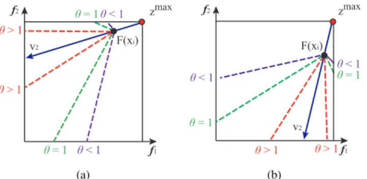
Now we consider the objective space. After normalization, the ideal point zmin becomes a zero vector, and the nadir point zmax = (zmax
1 , z2max, . . . , zmaxm )T can be constructed by finding the maximum value for each objective. For each individual xi inP, we consider two search directionsv1 and
v2 along whichF(xi)approaches to the PF. As shown in Fig.
1 (a), v1 = zmin −F(xi) and v2 = F(xi)−zmax. Along these directions, a solution set S is constructed by selecting promising solutions from both P and Q with the help of a binary directions selectionprocedure (line 2 in Algorithm2).
f2 v F(xi) PF min z 1 f1 v2 max z (a) f2 v a d2 F(xi) F(y) PF min z 1 F(y') a1 f1 (b)
Fig. 1. Illustrations of two search directions [Fig. 1(a)], and thescalar projectiona1[Fig.1(b)].
As will be shown in III-C, the number of solutions in S is 2N. Therefore, some technique is needed to prune the population S so as to retain exactly N solutions. In PAEA, the elimination function (line 3 in Algorithm 2) is designed for this purpose, where effective techniques are developed to handle extreme solutions and to eliminate solutions one by one. More details of this procedure will be given in Section
III-D. f2 v a d2 F(xi) F(y) PF min z 1 F(y') a1 f1 d1 d'1 (a) f2 v a d2 F(xi) F(y) PF max z 2 F(y') a1 f1 d1 d' 1 (b)
Fig. 2. Illustrations of the calculation ofg1(y|v1,zmin)[Fig.2(a)] and g2(y|v2,zmax)[Fig.2(b)].
C. Binary Directions Selection
As its name suggests, the binary directions selection chooses elite individuals in two directions in terms of the fitness value of an individual. A crucial issue here is how to measure the quality of individuals. Ideally, the fitness of an individual should reflect information concerning both convergence and diversity. As shown in Fig. 1 (b), a is a vector starting from F(xi) and ending up with F(y), where y is one of xi’s two children. On one hand, a1, given by ∥a∥ cos⟨a,v1⟩, where
⟨a,v1⟩ denotes the angle between a and v1, is called the
scalar projection of a onto the direction v1. The larger the
a1 is, the closer theF(y) approaches to the PF. Inversely, if
we consider the negative value ofa1, i.e.,−a1, then a smaller
value is preferable. Thus,−a1can be used as a measurement
of convergence for an individual. On the other hand, since the diversity of the parent population is well kept by using an angle-based strategy (which will be described in Section
III-D), we expect the offspring with better convergence is close to its parent. To this end, the perpendicular distance d2 from
F(y)tov1 can be used as a diversity measurement.
Therefore, for an individualy, its convergence and diversity (in the direction ofv1) are measured by −a1 andd2,
respec-tively. Thus, the fitness ofy can be defined as
g1(y|v1,zmin) = (−a1) +θ d2 (2)
where θ > 0 is a control parameter that is used to keep a balance between convergence and diversity. Actu-ally, Eq. (2) can be represented by two PBI functions as gpbi(y|v
1,zmin)−gpbi(xi|v1,zmin), where gpbi(y|v1,zmin)
and gpbi(x
i|v1,zmin) are the fitness value of y and xi in the directionv1according to the PBI decomposition approach
[21]. As shown in Fig.2(a),d1is the distance betweenzmin
andF(y′), i.e., the projection ofF(y)onv1;d2is the distance
betweenF(y)andF(y′);d′1is the distance between zmin and
F(xi).
Therefore, according to Fig.2(a), we have g1(y|v1,zmin) =−a1+θ d2 = (d1−d ′ 1) +θd2 = (d1+θd2)−(d ′ 1+θ·0)
=gpbi(y|v1,zmin)−gpbi(xi|v1,zmin)
(3) Algorithm 3 S←binaryDirectionsSelection(P, Q) Input: P, Q Output: S 1: S ← ∅ 2: foreach xi ∈P do
3: Calculate fitness values ofxiand its two child solutions y1 andy2 by Eqs. (3) and (4)
4: Two solutions y′1 and y′2 with the smallest values on each fitness function [Eqs. (3) and (4)] are selected from the set {xi,y1,y2}
5: if y′1=y′2 then
6: Select the solution with the second best value on eitherg1 org2, and use it to replacey′2//g1 org2 is
chosen randomly with a probability 0.5
7: end if
8: S←S∪ {y′1,y2′} // Addy′1 andy′2 intoS 9: end for
10: return S
Similarly, the fitness ofy, denoted byg2(y|v2,zmax), can be
also calculated in the directionv2by usingzmaxas a reference
point. According to Fig. 2 (b), this fitness value is actually the differences between two inverted PBI (IPBI) functions [41]. According to [41], the scalar optimization problem of IPBI function is defined by M aximize gipbi(y|v2,zmax) =
d1−θd2.In this paper, we consider the minus version, namely,
M inimize gipbi(y|v2,zmax) = −d1 +θd2. Therefore, we
obtain g2(y|v2,zmax) =−a1+θ d2 =−(d1−d ′ 1) +θd2 = (−d1+θd2)−(−d ′ 1+θ·0)
=gipbi(y|v2,zmax)−gipbi(xi|v2,zmax)
f2 θ > 1 min z f1 θ > 1 θ = 1 θ = 1 θ < 1 θ < 1 F(xi) v1 (a) f2 θ > 1 min z f1 θ > 1 θ = 1 θ = 1 θ < 1 θ < 1 F(xi) v1 (b)
Fig. 3. Contour lines ofg1(y|v1,zmin)with different values ofθ, shown
in a 2-objective space. f2 θ > 1 max z f1 θ > 1 θ = 1 θ = 1 θ < 1 θ < 1 v2 F(xi) (a) f2 θ > 1 max z f1 θ > 1 θ = 1 θ = 1 θ < 1 θ < 1 F(xi) v2 (b)
Fig. 4. Contour lines ofg2(y|v2,zmax)with different values ofθ, shown
in a 2-objective space.
For the fitness defined by Eqs. (3) and (4), a small value is preferable. With these fitness assignments, as shown in Algorithm 3, the binary directions selection procedure works as follows. For one parent solutionxi and its two child solu-tions y1 andy2, based ong1(y|v1,zmin)andg2(y|v2,zmax),
two solutions with the best (smallest) values on each fitness function are selected (lines 3 and 4 in Algorithm 3). In case that they are identical,y′2will be replaced by the solution with the second best value on either g1 or g2, which is randomly
chosen with a probability 0.5 (lines 5-7 in Algorithm3). The selectedy′1andy′2are added into the setS(line 8 in Algorithm
3)
Finally, we analyze the search behaviors of PAEA in depth by showing contour lines of both g1(y|v1,zmin) and
g2(y|v2,zmax), which are given in Figs.3and4, respectively.
According to Eq. (3), the second part gpbi(x
i|v1,zmin) is
fixed for different y’s, which is actually equal to the dis-tance between F(xi) and zmin. Therefore, the contour lines of g1(y|v1,zmin) is similar to those of gpbi(y|v1,zmin). To
be more specific, as shown in Fig. 3, the contour lines of g1(y|v1,zmin)are symmetrical about the search directionv1,
with the angle between the two lines larger than, equal to and smaller thanπ/2forθ <1,θ= 1andθ >1, respectively. S-inceg1(xi|v1,zmin) =gpbi(xi|v1,zmin)−gpbi(xi|v1,zmin) = 0, solutions on the contour line have the sameg1 value (i.e.,
g1= 0) as the current solutionxi. In Fig.3(a), solutions in the
region surrounded by the two contour lines of the sameθand the two axes haveg1 value smaller than 0. Thus, solutions in
this region are better than xi. Hence, by using the function g1, the current population is pulled toward the ideal point
zmin as close as possible. In a similar way, the contour lines of g2(y|v2,zmax) can be analyzed. As shown in Fig. 4, the
positive effect of the fitness function g2 is that it pushes the
current population toward the PF so as to make solutions in the population away from the nadir pointzmaxas far as possible. Moreover, as shown in Fig. 3 (a) and (b), if we use only g1 (or equally zmin), all the solutions are pulled toward the
ideal point, leading to over-crowdedness at middle parts of the PF in case that the problems have convex PFs (Note in this case, as shown in Fig. 4 (a) and (b), the use of g2 (or
equallyzmax) would be helpful for finding more solutions in the boundary). Similar problem occurs if we use onlyg2for a
concave PF [36]. Therefore, the simultaneous use of both g1
and g2 is likely to improve the performance of PAEA when
approximating both convex and concave PFs. The effect of the binary directions selection will be verified experimentally in Section VI-A of the supplementary materials.
D. Elimination procedure
Since S contains 2N solutions, an elimination procedure is needed to prune the population so as to retain exactly N solutions for the next generation. In PAEA, an angle-based procedure is used for this purpose, which is shown in Algorithm 4. The procedure is made up of two main parts: the handling of extreme solutions and the elimination of non-extreme solutions. Before the procedure starts, the acute angle (in the objective space) of every two individuals in S is calculated and stored in a matrixM2N×2N, and this operation needsO(mN2)multiplications. For every member inS, it has
a unique identity. With the help of the angle matrixM2N×2N and the identities of individuals, the angle between any two individuals can be obtained in the time complexity ofO(1). Algorithm 4 P′ ←elimination(S)
Input: S
Output: The new population P′
1: P′← ∅
2: Addm extreme solutions intoP′ and remove them from S
3: while |P′|+|S|> N do
4: Find xr and xt that have the minimum angle to each other among all the pairs of individuals in S
5: x ← arg max{∥F(xr)∥,∥F(xt)∥} // Find the worse individual x in terms of the length of the objective vectors
6: Remove x fromS
7: end while
8: P′←P′∪S
9: return P′
For each objective k, we define a unit vector ek =
(0, . . . ,1, . . . ,0), where the kth element is 1 and all the other ones are 0’s. For this vector, in the objective space, find the solution xk to which ek has the minimum angle. The xk is called anextreme solution. The inclusion of extreme solutions may be good for the diversity promotion. However, some extreme solutions may be far away from the true PF. This will
have a side effect on the convergence of the whole population if these poorly converged solutions are directly included.
To handle the above problem, the following strategy is used in the proposed algorithm (refer to line 2 in Algorithm4). First, find out the individualsxk andxh that have the minimum and the second minimum angle toek. Second, a choice betweenxk andxh is made according to the length of their objective vec-tors. The ∥F(xk)∥is the distance from F(xk)tozmin, which can reflect the convergence of the individualxk. The selection logic is as follows: if ∥F(xk)∥ − ∥F(xh)∥ ≤α∥F(xh)∥, then xk is added intoP′, and is also removed fromS. Otherwise, xh is selected. Note that a parameter α > 0 is used in the selection condition. According to this selection strategy, if F(xk) is extremely far away from the true PF, then it would not be included in the new population. Hence, the diversity and convergence can be balanced when adding extreme solutions. For the remaining individuals in S, we first find out a pair of solutions, denoted byxr andxt, which have the minimum angle among all the pairs of individuals (line 4 in Algorithm
4). Then, we identify the worse one (denoted byx) in terms of the length of the objective vectors (line 5 in Algorithm4). In case that a “tie” occurs, it will be broken randomly. Next,xis removed fromS(line 6 in Algorithm4). The above procedure is repeated if|P′|+|S|> N, where|·|is the cardinal number of a set. Finally, Algorithm4 returns the union ofP′ andS. It should be noted that He and Yen [53] have recently proposed a similar procedure to eliminate solutions one by one. Each time their procedure finds a pair of individuals with the minimum angle. If the difference of two closest solutions’ Euclidean distance is larger than a predefined threshold value t, then the one with the larger Euclidean distance to the ideal point is eliminated. Otherwise, the one with a smaller angle to other solutions is removed. In practice, the value of the parametertshould be set carefully according to characteristics of the problems at hand [53]. Our procedure, however, ignores the use of the parameter t. In addition, we here present a fast implementation of the above elimination procedures. Naively, the time complexity of lines 3-7 in Algorithm4isO(N3). In
each of the N loops, we need to find a pair of solutions with the minimum angle to each other from all theO(N2)pairs of
solutions. Actually, lines 3-7 in Algorithm 4 can be speeded up by the following routine. First, we have the following preprocessing: sorting angle values of all pairs of solutions in an ascending order by using Quicksort [54]. Since there are
(2N−m
2
)1
= (2N−m)(22N−m−1) = O(N2) pairs of solutions,
this requires O(N2logN2) = O(N2logN) comparisons by
using Quicksort. After sorting, the minimum angle can be found in the first place of the angle array. We delete one of the two solutions associated with this angle according to lines 5 and 6 in Algorithm4. Subsequently, the angles related to the deleted solution should be removed from the array. From a programmatic perspective, this can be done by setting these angles to a large number (e.g., M). Note that, for each solution, the array indexes of angles related to this solution can be recorded during the quick sort process. Therefore, the
1Sincem extreme solutions are removed fromS according to line 2 of
Algorithm4, there are exactly2N−mremaining solutions inS.
marking of these angles needs only O(N) operations. Then, the procedure continues scanning the array and the first angle that is not equal toM is the second minimum angle. Similarly, an associated solution is removed, so do angles related to this solution. The above procedures are repeated untilN solutions are removed. Therefore, the routine needsO(N2)deletions of
angles (by marking them with M), and O(N2) scans of the
angle array. AsO(N2logN)is larger thanO(N2), the worst time complexity of the above routine is O(N2logN), which is lower thanO(N3).
The overall worst-case time complexity of PAEA at one gen-eration ismax{O(N2logN), O(mN2)}. For detailed analyses and comparisons, we direct readers to Section V of the sup-plementary materials. Moreover, we give some discussions on the differences/relations between PAEA and related algorithms in Section I of the supplementary materials.
IV. EXPERIMENTALSTUDY
In this section, the proposed PAEA is compared with MOEA/DD [9], NSGA-III [8], MOEA/D [21], 1by1EA [55], GWASF-GA [42], MOEA/D-AWA [39] and MOEA/D-TPN [43] on a large number of test problems. These state-of-the-art algorithms were demonstrated to be effective when handling MaOPs. All the algorithms, except for 1by1EA, are reference point/weight vector based approaches. Similar to PAEA, the 1by1EA does not require any predefined weight vector. Since PAEA uses both ideal and nadir points, we include 1by1EA, GWASF-GA and MOEA/D-TPN as peer algorithms as they also use the two reference points in different ways.
A. Test Problems
In the empirical study, we consider 32 test problems that are selected from two test suites. One is the DTLZ test suite con-sisting of 14 problems: DTLZ1−DTLZ7 [56], ConvexDTLZ2 [8], ScaledDTLZ1-2 [8] and DTLZ1−1−DTLZ4−1 [24]. The
other is the WFG test suite containing 18 test problems: WFG1−WFG9 [57] and WFG1−1−WFG9−1[24]. All the test problems can be scaled to any number of objectives. In this paper, m= 5,8,10and15are considered.
In all the experiments, the number of decision variables for DTLZ test problems is set to n = m+k−1, where k = 5 for DTLZ1 and ScaledDTLZ1, k = 20 for DTLZ7 and k = 10 for other DTLZ test problems [56]. According to suggestions in [57], the number of decision variables in WFG test problems is set to n = 2×(m−1) +l, where l is the distance-related variable that is set to 20. Recently, Ishibuchi et al. [24] have proposed the DTLZ−1 and WFG−1
test problems which are minus versions of DTLZ and WFG, respectively. The minus problems are created by multiplying all objectives in the original DTLZ and WFG by (-1). In this paper, the settings of decision variables and objectives are the same as in the original DTLZ and WFG test problems.
B. Performance Metrics
In this paper, the inverted generational distance (IGD) [58], [59], the generational distance (GD) [60] and the pure
diversity (PD) [30] are chosen as performance metrics. The IGD can provide combined information on convergence and diversity of the obtained solutions, therefore it is widely used in the evaluation of approximated solution sets for both MOPs [58], [61], [62] and MaOPs [8]–[10], [23], [49], [63]. The GD assesses only the convergence while PD gives a pure measurement on the diversity.
When calculating both IGD and GD, a reference point set is needed. In this paper, the same method as in [64] is used to sample points on the true PF. For more details, please refer to Section II-A of the online supplementary materials. For both IGD and GD, small values are preferable. The PD is a recently proposed diversity assessment in many-objective optimization. Details of the calculation of PD can be found in [30]. It is worth mentioning that an approximate set that is far away from the true PF may also present a satisfactory PD result if solutions are distributed properly. However, this PD value may be meaningless and may lead to misleading results. To avoid this situation, PD values in this paper are calculated only among those solutions whose objective values are within the regions of the true PF. Thus, worse converged solutions in any objective contribute zero to the PD value. In this way, the PD metric can also measure the convergence to some extent. For PD metric, a large value is desirable. In the study, this metric is implemented by the code2 provided in [30].
C. General Experimental Settings
The experimental settings in this study are listed below unless otherwise mentioned.
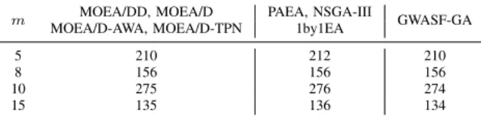
• Population sizeN:According to [8], the population size in NSGA-III is set to the smallest multiple of four larger than the number of weight vectors (denoted byH), which are created by the Das and Dennis’s systematic approach [50] whenm= 5 and by the two-layer weight/reference vectors generation method [8], [9] whenm >5. In PAEA and 1by1EA, the population size keeps the same as in NSGA-III. While in MOEA/DD, MOEA/D, MOEA/D-AWA and MOEA/D-TPN, the population size is set toH directly. For GWASF-GA, N is set to H when m = 5 and 8, and H−1when m=10 and 15. Since a binary tournament selection is used in GWASF-GA, it requires the population size to be even. In case that the number of generated weight vectors is odd, a random one will be removed as done in [42]. The values of N for different numbers of objectives are summarized in Table I.
TABLE I
THE POPULATION SIZENFOR DIFFERENT NUMBERS OF OBJECTIVES
m MOEA/DD, MOEA/D PAEA, NSGA-III GWASF-GA MOEA/D-AWA, MOEA/D-TPN 1by1EA
5 210 212 210
8 156 156 156
10 275 276 274
15 135 136 134
2The code of PD can be found at http://www.surrey.ac.uk/cs/people/ handing wang/
TABLE II
THE SETTINGS OF THEmaxF EsFOR DIFFERENT NUMBERS OF
OBJECTIVES ON EACH TEST PROBLEM.
m DTLZ1 DTLZ2 DTLZ3 DTLZ4 Others
5 212×600 212×350 212×1000 212×1000 212×1250 8 156×750 156×500 156×1000 156×1250 156×1500 10 276×1000 276×750 276×1500 276×2000 276×2000 15 136×1500 136×1000 136×2000 136×3000 136×3000
• The number of independent runs and the termination condition:All algorithms are independently run 30 times in each test instance, and are terminated when the objec-tive function evaluations reachmaxF Es. The settings of maxF Esfor different numbers of objectives on each test problem are summarized in Table II.
• Algorithmic parameter settings: In our proposed PAEA, there are two additional parameters θ andα, which are set to 10 and 0.5, respectively. The parameter study on θ andαis available in Section IV of the supplementary materials. For other peer algorithms, the parameter set-tings are kept the same as in their original studies. More details can be found in Section II-B of the supplementary materials.
D. Comparison of Computational Results
For performance comparisons, we first record the average IGD and PD for the DTLZ test suite as shown in Tables II and III of the supplementary materials. As we can see from these tables, PAEA obtains the best or the second best results in most of the test instances, showing a great superiority over other state-of-the-art algorithms. Specifically, among all the 56 DTLZ and DTLZ−1 test instances, the proportion of the
best or the second best results PAEA obtains is34/56≈61%
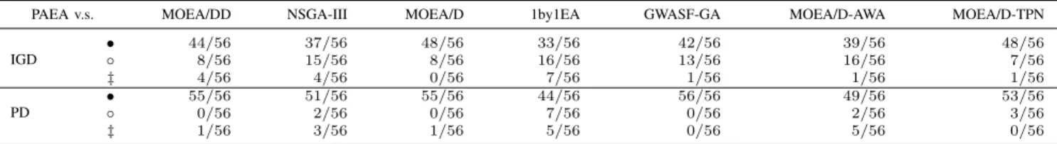
and 52/56 ≈ 93% for IGD and PD, respectively. To make statistical comparisons, the Wilcoxon’s rank sum test [65] is applied to determining whether the differences between PAEA and each peer algorithm in each test instance are significant or not. The symbol• denotes that PAEA shows a significant improvement over its competitors with a level of significance α = 0.05, while ◦ indicates the opposite. If no significant difference is found, then the symbol ‡will be used. The test results on DTLZ test suite are summarized in TableIII, where we can find the proportion of test instances where PAEA is better than (•), worse than (◦) and equal to (‡) each of the peer algorithms.
It can be observed from Table III that the proportion of the DTLZ and DTLZ−1 test instances where PAEA obtains
significantly better IGD than its competitors is44/56,37/56,
48/56, 33/56, 42/56, 39/56 and 48/56 for MOEA/DD, NSGA-III, MOEA/D, 1by1EA, GWASF-GA, MOEA/D-AWA and MOEAD-TPN, respectively. Conversely, the proportion of test instances where PAEA is inferior to the peer algorithms is8/56,15/56,8/56,16/56,13/56,16/56and7/56, respec-tively. For the PD metric, as shown in TableIII, PAEA outper-forms GWASF-GA in all the 56 test instances, and outperoutper-forms both MOEA/DD and MOEA/D in 55 test instances. Compared with NSGA-III, 1by1EA, MOEA/D-AWA and MOEAD-TPN,
TABLE III
THE PROPORTION OFDTLZANDDTLZ−1TEST INSTANCES WHEREPAEAIS BETTER THAN(•),WORSE THAN(◦)AND EQUAL TO(‡)EACH OF
THE PEER ALGORITHMS ACCORDING TO THEWILCOXON’S RANK SUM TEST.
PAEA v.s. MOEA/DD NSGA-III MOEA/D 1by1EA GWASF-GA MOEA/D-AWA MOEA/D-TPN
IGD • 44/56 37/56 48/56 33/56 42/56 39/56 48/56 ◦ 8/56 15/56 8/56 16/56 13/56 16/56 7/56 ‡ 4/56 4/56 0/56 7/56 1/56 1/56 1/56 PD • 55/56 51/56 55/56 44/56 56/56 49/56 53/56 ◦ 0/56 2/56 0/56 7/56 0/56 2/56 3/56 ‡ 1/56 3/56 1/56 5/56 0/56 5/56 0/56 TABLE IV
THE PROPORTION OFWFGANDWFG−1TEST INSTANCES WHEREPAEAIS BETTER THAN(•),WORSE THAN(◦)AND EQUAL TO(‡)EACH OF THE
PEER ALGORITHMS ACCORDING TO THEWILCOXON’S RANK SUM TEST.
PAEA v.s. MOEA/DD NSGA-III MOEA/D 1by1EA GWASF-GA MOEA/D-AWA MOEA/D-TPN
IGD • 70/72 52/72 68/72 57/72 44/72 49/72 64/72 ◦ 1/72 16/72 1/72 3/72 23/72 23/72 6/72 ‡ 1/72 4/72 3/72 12/72 5/72 0/72 2/72 PD • 71/72 67/72 71/72 68/72 72/72 62/72 66/72 ◦ 1/72 4/72 1/72 3/72 0/72 8/72 3/72 ‡ 0/72 1/72 0/72 1/72 0/72 2/72 3/72
PAEA obtains better PD in 51,44, 49and 53out of 56 test instances, respectively.
The raw experimental results on the WFG test suite are provided in Tables IV and V of the supplementary materials. To have a preliminary understanding of the comparisons, main statistics are summarized as follows: among all the 72 WFG and WFG−1 test instances, the proportion of the best or the second best results PAEA obtains is 50/72 ≈ 69%
and 67/72 ≈ 93% for IGD and PD, respectively. To make the comparisons easier, the Wilcoxon’s rank sum test results are summarized in Table IV where we can find that the largest and smallest proportion of WFG and WFG−1 test
instances where PAEA performs better in terms of IGD is
70/72 ≈ 97% (PAEA v.s. MOEA/DD) and 44/72 ≈ 61%
(PAEA v.s. GWASF-GA), respectively. Similarly, the largest proportion of test instances where PAEA obtains better PD values is 72/72 = 100% (PAEA v.s. GWASF-GA), and the smallest proportion is 62/72 ≈ 86% (PAEA v.s. MOEA/D-AWA). It is clear from the table that PAEA shows significantly better performance than other state-of-the-art algorithms in the majority of the test instances. Intuitive comparisons of the distribution of the final solutions are provided in Section III of the supplementary materials. As a summary, it can be found from these materials that the solutions of PAEA are distributed more widely than those of its competitors.
V. DISCUSSIONS
In this section, we explain in depth why the state-of-the-art algorithms perform as they do. For MOEA/DD and MOEA/D, they perform competitively on normalized problems (e.g., DTLZ1-4), but degenerate on problems with differently scaled objective functions (e.g., ScaledDTLZ1-2, WFG1-9, WFG1-9−1). In MOEA/D, a new solution is generated for a
weight vector by selecting parents from the neighbors. The new solution is compared with all of its neighbors. If the new solution is better, then the current solution is replaced. Hence, there is a risk that many neighboring solutions are replaced by a same good solution. This will do harm to the diversity of the solutions [24], which is reflected by the parallel
coordinates as shown in Fig. 1 (d), Fig. 2 (d) and Fig. 3 (d) of the supplementary materials. The MOEA/DD performs not well on the WFG test problems, and this may be due to the lack of an efficient objective normalization mechanism in MOEA/DD [24]. For GWASF-GA, it performs poorly in terms of the diversity of obtained solutions on the original DTLZ and WFG test problems. As stated in [42], the final population of GWASF-GA depends highly on the distribution of the weight vectors used. In GWASF-GA, the weight vectors are predefined and are not recalculated as the generations are increased. As a result, the algorithm cannot dynamically adapt the evolution of the population to the shapes of the PF.
The NSGA-III is significantly worse than PAEA in terms of the PD metric. This may be explained as follows. Since the majority of solutions in a high-dimensional objective space are non-dominated with each other, they fall into the same layer according to the non-dominated sorting procedure adopted by NSGA-III. When this primary selection criterion fails to distinguish individuals, the reference line based diversity preservation strategy is activated. However, it is possible that some reference lines have multiple solutions, while other reference lines have no solutions [24]. In addition, the refer-ence points generated by the two-layer approach in NSGA-III are mainly distributed on two layers of the hyper-plane [8]. Therefore, solutions found by NSGA-III concentrate mainly on the boundary or middle parts of the true PF. Hence, worse PD values are obtained by NSGA-III compared with PAEA.
The 1by1EA is highly competitive with the proposed PAEA on the DTLZ test suite. The algorithm selects individuals one-by-one based on convergence indicators in the environmental selection. Once a solution is selected, its neighbors are de-emphasized using a niche technique to guarantee the diversity of the population. Hence, a good balance between convergence and diversity may be obtained. However, the performance of 1by1EA is related to the convergence indicators used. The 1by1EA prefers the convergence indicator whose contour lines have a similar shape to that of the PF of a given problem. Unfortunately, the shape of the PF of a practical optimization problem is usually unknown in advance. Therefore, the
en-hancements of 1by1EA may be possible by adaptively choos-ing an appropriate convergence indicator or uschoos-ing an ensemble of multiple convergence indicators during the evolution of the algorithm [55].
The MOEA/D-AWA performs competitively with PAEA on both DTLZ and WFG test suites with respect to both IGD and PD metrics. The success of MOEA/D-AWA may be attributed to the adaptive weight vector adjustment, which deletes overcrowded weight vectors and adds new ones into the sparse regions. Hence, the diversity among solutions is promoted. Thanks to this effective diversity maintenance strategy, MOEA/D-AWA obtains competitive IGD and PD results compared with PAEA. However, since MOEA/D-AWA maintains an external population and needs to calculate the crowdedness of solutions, it requires more computational costs. As shown in Section V of the supplementary materials, MOEA/D-AWA runs slowest among all the peer algorithms.
The MOEA/D-TPN was demonstrated to be promising when handling 2- and 3-objective MOPs with complex PFs [43], which is also verified by our experimental results on test functions F1-F9 [36] as shown in Section III of the supple-mentary materials. However, the performance of MOEA/D-TPN degenerates on many-objective problems. One possible reason for the performance deterioration is that MOEA/D-TPN is sensitive to some key control parameters. Different settings of these parameters may be required for MaOPs. As another likely explanation, MOEA/D-TPN uses fixed weight vectors, being unable to adapt to the shapes of the PFs.
As can be found from the experimental results, the perfor-mance of MOEA/D, MOEA/DD and NSGA-III degrades on DTLZ−1and WFG−1test problems. As explained in [24], this
performance deterioration is attributed to the inconsistencies between the shapes of the PFs and those of the weight vectors used in these algorithms. For our proposed PAEA, however, it performs well on both DTLZ/DTLZ−1 and WFG/WFG−1
test problems. First, PAEA uses adaptive search directions such that it can handle problems with irregular PFs, such as DTLZ5-6 and WFG3. Second, each solution in PAEA is simultaneously evaluated on two fitness functions taking into account different reference points. Therefore, PAEA can take advantages of the complementary effects of both ideal and nadir points for either concave or convex PFs. Besides, the diversity among solutions in the environmental selection is maintained by an angle-based one-by-one elimination proce-dure. Finally, some other techniques, such as the adaptive normalization of the population and a smart procedure for including extreme solutions are also factors for the success of our proposed PAEA. For further discussions on PAEA, we direct readers to Section VI of the supplementary materials.
VI. CONCLUSION ANDFUTUREWORK
This paper proposes a new decomposition-based many-objective optimizer, i.e., PAEA, by using two primary con-cepts: scalar projection and angle. In PAEA, search directions are defined based on the current solutions and two refer-ence points. For each solution, binary search directions are considered. One is the direction from the current individual
to the ideal point, while the other is from the nadir point to the current solution. The scalar projection motivates us to develop two fitness functions, which are deduced to be the differences between two PBI functions and two IPBI functions, respectively. Each individual is then evaluated on the two fitness functions simultaneously, and solutions with the best values on each function are emphasized. Finally, the angle information is adopted to select diversified solutions for the next generation. The proposed PAEA is compared with seven state-of-the-art algorithms on a large number of test problems. As shown in the experimental study, PAEA obtains promising results on these test problems with up to 15 objectives, regarding both the quality of the final solutions and the efficiency of the algorithm.
Major advantages of PAEA are that: 1) it uses adaptive search directions, therefore problems with irregular PFs could be effectively handled; 2) PAEA uses two fitness functions with different reference points to distinguish individuals, hence it takes advantages of the complementary effects of both ideal and nadir points. Consequently, PAEA is able to properly deal with problems with both concave and convex PFs. A potential shortcoming of PAEA would be that it currently considers only the distance to the ideal point as the convergence metric when eliminating solutions one by one as shown in Algorithm 4. Actually, other convergence metrics [55] could be used, which will be one of our future studies. As another meaningful research direction, besides the angle-based clustering method developed in this paper (see Section VI-B in the supplementary materials), it is possible to use ideas from other related works [66]–[69] to match between parents and offspring so as to further improve the performance of the proposed algorithm. In addition, applying PAEA to imbalanced problems [70], [71] or problems from practice would be also one of our subsequent research subjects.
ACKNOWLEDGMENT
The authors would like to thank the Associate Editor and the anonymous reviewers for providing valuable comments to improve this paper. We also add thanks to Dr. X. He (Sun Yat-Sen University) for his helpful discussions when preparing the revisions of the paper.
REFERENCES
[1] M. Farina and P. Amato, “On the optimal solution definition for many-criteria optimization problems,” inAnnual Meeting of the North American Fuzzy Information Processing Society. IEEE, 2002, pp. 233– 238.
[2] B. Li, J. Li, K. Tang, and X. Yao, “Many-objective evolutionary algorithms: A survey,” ACM Computing Surveys, vol. 48, no. 1, pp. 1–35, Sep 2015.
[3] R. J. Lygoe, M. Cary, and P. J. Fleming, “A Real-World Application of a Many-Objective Optimisation Complexity Reduction Process,” in Evo-lutionary Multi-criterion Optimization, ser. Lecture Notes in Computer Science, vol. 7811. Springer, 2013, pp. 641–655.
[4] E. Matrosov, “Using many-objective optimization and robust decision making to identify robust regional water resource system plans,” in2015 AGU Fall Meeting. Agu, 2015.
[5] K. Narukawa and T. Rodemann, “Examining the performance of evolutionary many-objective optimization algorithms on a real-world application,” in Genetic and Evolutionary Computing (ICGEC), 2012 Sixth International Conference on. IEEE, 2012, pp. 316–319.
[6] Y. Xiang, Y. Zhou, Z. Zheng, and M. Li, “Configuring Software Product Lines by Combining Many-Objective Optimization and SAT Solvers,”
ACM Trans. Softw. Eng. Methodol., vol. 26, no. 4, pp. 14:1–14:46, Feb. 2018.
[7] M. Li, S. Yang, and X. Liu, “Bi-goal evolution for many-objective optimization problems,” Artificial Intelligence, vol. 228, pp. 45–65, 2015.
[8] K. Deb and H. Jain, “An evolutionary many-objective optimization algorithm using reference-point based nondominated sorting approach, part I: Solving problems with box constraints,”IEEE Transactions on Evolutionary Computation, vol. 18, no. 4, pp. 577–601, 2014. [9] K. Li, K. Deb, Q. Zhang, and S. Kwong, “An evolutionary
many-objective optimization algorithm based on dominance and decomposi-tion,”IEEE Transactions on Evolutionary Computation, vol. 19, no. 5, pp. 694–716, Oct 2015.
[10] S. Yang, M. Li, X. Liu, and J. Zheng, “A grid-based evolutionary algorithm for many-objective optimization.”IEEE Transactions on Evo-lutionary Computation, vol. 17, no. 5, pp. 721–736, 2013.
[11] J. Bader and E. Zitzler, “HypE: An Algorithm for Fast Hypervolume-Based Many-Objective Optimization,” Evolutionary Computation, vol. 19, no. 1, pp. 45–76, Jul. 2011.
[12] D. Gong, J. Sun, and Z. Miao, “A set-based genetic algorithm for interval many-objective optimization problems,”IEEE Transactions on Evolutionary Computation, vol. PP, no. 99, pp. 1–1, 2017.
[13] Y. Liu, D. Gong, X. Sun, and Y. Zhang, “Many-objective evolution-ary optimization based on reference points,”Applied Soft Computing, vol. 50, no. Supplement C, pp. 344 – 355, 2017.
[14] Y. Xiang, Y. Zhou, L. Tang, and Z. Chen, “A decomposition-based many-objective artificial bee colony algorithm,”IEEE Transactions on Cybernetics, vol. PP, no. 99, pp. 1–14, 2017.
[15] Z. Chen, Y. Zhou, and Y. Xiang, “A many-objective evolutionary algorithm based on a projection-assisted intra-family election,”Applied Soft Computing, vol. 61, pp. 394–411, 2017.
[16] K. Deb, Multi-objective optimization using evolutionary algorithms. John Wiley & Sons, 2001, vol. 16.
[17] A. Zhou, B.-Y. Qu, H. Li, S.-Z. Zhao, P. N. Suganthan, and Q. Zhang, “Multiobjective evolutionary algorithms: A survey of the state of the art,”Swarm and Evolutionary Computation, vol. 1, no. 1, pp. 32 – 49, 2011.
[18] E. Zitzler, M. Laumanns, and L. Thiele, “SPEA2: Improving the strength pareto evolutionary algorithm,” Computer Engineering and Networks Laboratory,Department of Electrical Engineering, Swiss Federal Institute of Technology (ETH) Zurich,Switzerland, Tech. Rep., 2001.
[19] K. Deb, A. Pratap, S. Agarwal, and T. Meyarivan, “A fast and elitist multiobjective genetic algorithm: NSGA-II,” IEEE Transactions on Evolutionary Computation, vol. 6, no. 2, pp. 182–197, 2002. [20] E. Zitzler and S. K¨unzli, “Indicator-based selection in multiobjective
search,” in Proc. 8th International Conference on Parallel Problem Solving from Nature, PPSN VIII. Springer, 2004, pp. 832–842. [21] Q. Zhang and H. Li, “MOEA/D: A multiobjective evolutionary algorithm
based on decomposition,”IEEE Transactions on Evolutionary Compu-tation, vol. 11, no. 6, pp. 712–731, 2007.
[22] Y. Zhou, Z. Chen, and J. Zhang, “Ranking vectors by means of the dominance degree matrix,” IEEE Transactions on Evolutionary Computation, vol. 21, no. 1, pp. 34–51, Feb 2017.
[23] M. Li, S. Yang, and X. Liu, “Pareto or Non-Pareto: Bi-Criterion Evolution in Multiobjective Optimization,”IEEE Transactions on Evo-lutionary Computation, vol. 20, no. 5, pp. 645–665, Oct 2016. [24] H. Ishibuchi, Y. Setoguchi, H. Masuda, and Y. Nojima, “Performance
of decomposition-based many-objective algorithms strongly depends on pareto front shapes,”IEEE Transactions on Evolutionary Computation, vol. 21, no. 2, pp. 169–190, April 2017.
[25] H. Ishibuchi, Y. Hitotsuyanagi, H. Ohyanagi, and Y. Nojima, “Effects of the existence of highly correlated objectives on the behavior of moea/d,” inEvolutionary Multi-Criterion Optimization. Springer, 2011, pp. 166– 181.
[26] I. Giagkiozis, R. C. Purshouse, and P. J. Fleming, “Generalized decom-position and cross entropy methods for many-objective optimization,”
Information Sciences, vol. 282, pp. 363–387, 2014.
[27] E. Zitzler and L. Thiele, “Multiobjective evolutionary algorithms: A comparative case study and the strength pareto approach,”IEEE Trans-actions on Evolutionary Computation, vol. 3, no. 4, pp. 257–271, 1999. [28] D. Brockhoff, T. Wagner, and H. Trautmann, “On the properties of the r2 indicator,” inProceedings of the 14th annual conference on Genetic and evolutionary computation. ACM, 2012, pp. 465–472.
[29] A. Auger, J. Bader, D. Brockhoff, and E. Zitzler, “Theory of the hypervolume indicator: optimal µ-distributions and the choice of the reference point,” in Proceedings of the tenth ACM SIGEVO workshop on Foundations of genetic algorithms. ACM, 2009, pp. 87–102. [30] H. Wang, Y. Jin, and X. Yao, “Diversity assessment in many-objective
optimization,”IEEE Transactions on Cybernetics, vol. PP, no. 99, pp. 1–13, 2016.
[31] M. Li, S. Yang, and X. Liu, “A performance comparison indicator for pareto front approximations in many-objective optimization,” in
Proceedings of the 2015 on Genetic and Evolutionary Computation Conference. ACM, 2015, pp. 703–710.
[32] R. Hern´andez Gomez and C. Coello Coello, “MOMBI: A new meta-heuristic for many-objective optimization based on the R2 indicator,” inEvolutionary Computation (CEC), 2013 IEEE Congress on. IEEE, 2013, pp. 2488–2495.
[33] R. Hern´andez G´omez and C. A. Coello Coello, “Improved Metaheuris-tic Based on the R2 Indicator for Many-Objective Optimization,” in
Proceedings of the 2015 on Genetic and Evolutionary Computation Conference. ACM, 2015, pp. 679–686.
[34] K. Bringmann, “Bringing order to special cases of klees measure problem,” in Mathematical Foundations of Computer Science 2013. Springer, 2013, pp. 207–218.
[35] M. Wagner and F. Neumann, “A fast approximation-guided evolutionary multi-objective algorithm,” inProceedings of the 15th annual conference on Genetic and evolutionary computation. ACM, 2013, pp. 687–694. [36] Z. Wang, Q. Zhang, H. Li, H. Ishibuchi, and L. Jiao, “On the use of two reference points in decomposition based multiobjective evolutionary algorithms,”Swarm and Evolutionary Computation, vol. 34, pp. 89 – 102, 2017.
[37] S. Jiang, Z. Cai, J. Zhang, and Y.-S. Ong, “Multiobjective optimization by decomposition with pareto-adaptive weight vectors,” in2011 Seventh International Conference on Natural Computation, vol. 3, July 2011, pp. 1260–1264.
[38] H. Jain and K. Deb, “An evolutionary many-objective optimization algorithm using reference-point based nondominated sorting approach, part II: Handling constraints and extending to an adaptive approach,”
IEEE Transactions on Evolutionary Computation, vol. 18, no. 4, pp. 602–622, 2014.
[39] Y. Qi, X. Ma, F. Liu, L. Jiao, J. Sun, and J. Wu, “MOEA/D with adaptive weight adjustment,”Evolutionary Computation, vol. 22, no. 2, pp. 231– 264, June 2014.
[40] R. Cheng, Y. Jin, M. Olhofer, and B. Sendhoff, “A reference vector guided evolutionary algorithm for many-objective optimization,”IEEE Transactions on Evolutionary Computation, vol. PP, no. 99, pp. 1–1, 2016.
[41] H. Sato, “Inverted PBI in MOEA/D and its impact on the search per-formance on multi and many-objective optimization,” inProceedings of the 2014 Annual Conference on Genetic and Evolutionary Computation. ACM, 2014, pp. 645–652.
[42] R. Saborido, A. B. Ruiz, and M. Luque, “Global wasf-ga: an evolution-ary algorithm in multiobjective optimization to approximate the whole pareto optimal front,”Evolutionary computation, 2016.
[43] S. Jiang and S. Yang, “An improved multiobjective optimization evolu-tionary algorithm based on decomposition for complex pareto fronts,”
IEEE transactions on cybernetics, vol. 46, no. 2, pp. 421–437, 2016. [44] M. Laumanns, L. Thiele, K. Deb, and E. Zitzler, “Combining
con-vergence and diversity in evolutionary multiobjective optimization,”
Evolutionary Computation, vol. 10, no. 3, pp. 263–282, Sep. 2002. [45] Y. Yuan, H. Xu, B. Wang, and X. Yao, “A new dominance relation
based evolutionary algorithm for many-objective optimization,” IEEE Transactions on Evolutionary Computation, vol. 20, no. 1, pp. 16–37, 2016.
[46] S. F. Adra and P. J. Fleming, “Diversity Management in Evolution-ary Many-Objective Optimization,”IEEE Transactions on Evolutionary Computation, vol. 15, pp. 183–195, 2011.
[47] M. Li, S. Yang, and X. Liu, “Shift-based density estimation for pareto-based algorithms in many-objective optimization,” IEEE Transactions on Evolutionary Computation, vol. 18, pp. 348–65, June 2014. [48] P. C. Roy, M. M. Islam, K. Murase, and X. Yao, “Evolutionary Path
Control Strategy for Solving Many-Objective Optimization Problem,”
IEEE Transactions on Cybernetics, vol. 45, no. 4, pp. 702–715, APR 2015.
[49] H. Wang, L. Jiao, and X. Yao, “Two Arch2: An Improved Two-Archive Algorithm for Many-Objective Optimization,” IEEE Transactions on Evolutionary Computation, vol. 19, pp. 524–541, August 2015. [50] I. Das and J. E. Dennis, “Normal-boundary intersection: A new method
![Fig. 1. Illustrations of two search directions [Fig. 1 (a)], and the scalar projection a 1 [Fig](https://thumb-us.123doks.com/thumbv2/123dok_us/808482.2602238/5.918.79.435.83.258/fig-illustrations-search-directions-fig-scalar-projection-fig.webp)