Quantized consensus ADMM for multi-agent distributed optimization

Conference Proceedings and Posters

2016

Quantized consensus ADMM for multi-agent

distributed optimization

Shengyu Zhu

Syracuse University

Mingyi Hong

Iowa State University, [email protected]

Biao Chen

Syracuse University

Follow this and additional works at:

http://lib.dr.iastate.edu/imse_conf

Part of the

Industrial Engineering Commons

,

Other Operations Research, Systems Engineering

and Industrial Engineering Commons

, and the

Systems Engineering Commons

This Conference Proceeding is brought to you for free and open access by the Industrial and Manufacturing Systems Engineering at Iowa State University Digital Repository. It has been accepted for inclusion in Industrial and Manufacturing Systems Engineering Conference Proceedings and Posters by an authorized administrator of Iowa State University Digital Repository. For more information, please [email protected].

Recommended Citation

Zhu, Shengyu; Hong, Mingyi; and Chen, Biao, "Quantized consensus ADMM for multi-agent distributed optimization" (2016).

Industrial and Manufacturing Systems Engineering Conference Proceedings and Posters. 49.

arXiv:1510.08736v1 [math.OC] 29 Oct 2015

Quantized Consensus ADMM for Multi-Agent

Distributed Optimization

Shengyu Zhu, Mingyi Hong, and Biao Chen

Abstract

Multi-agent distributed optimization over a network minimizes a global objective formed by a sum of local convex functions using only local computation and communication. We develop and analyze a quantized distributed algorithm based on the alternating direction method of multipliers (ADMM) when inter-agent communications are subject to finite capacity and other practical constraints. While existing quantized ADMM approaches only work for quadratic local objectives, the proposed algorithm can deal with more general objective functions (possibly non-smooth) including the LASSO. Under certain convexity assumptions, our algorithm converges to a consensus within log1+ηΩ iterations, whereη > 0 depends on the local objectives and the network topology, and Ω is a

polynomial determined by the quantization resolution, the distance between initial and optimal variable values, the local objective functions and the network topology. A tight upper bound on the consensus error is also obtained which does not depend on the size of the network.

Index Terms

Multi-agent distributed optimization, quantization, alternating direction method of multipliers (ADMM), linear convergence.

I. INTRODUCTION

T

HERE has been much research interest in distributed optimization due to recent advances in networked multi-agent systems [1], [2]. For example, ad hoc network applications may require multi-agents to reach a consensus on the average of their measurements [3], including distributed coordination of mobile autonomous agents [4], and distributed data fusion in sensor networks [5]. Another example is the large scale machine learning where a computation task may be executed by collaborative microprocessors with individual memories and storage spaces

[6], [7]. Many of the distributed optimization problems, such as those mentioned, can be cast as an optimization problem of the following form

min ˜ x N X i=1 fi(˜x), (1)

where fi :RM →R∪ {∞}is the local objective function associated with agent i. The function fi is composed of

a smooth component gi:RM →R∪ {∞} and a non-smooth componenthi :RM →R∪ {∞}, i.e., fi=gi+hi.

Examples of such models include least squares [8], [9] and regularized least squares [10]–[12]. The variable x˜

may represent average temperature of a room [5], frequency-domain occupancy of spectra [12], states of smart grid systems [13], etc.

In the above scenarios, it is commonly assumed that each agent only has the knowledge of its local objective function, and a fusion center is either disallowed or not economical. As such, the agents seek to solve (1) collaboratively using only local computation and communication. In practice, a number of factors, such as limited bandwidth, sensor battery power, and computing resources, place tight constraints on the rate and form of information exchange amongst neighboring agents, resulting in the quantized communication constraint. The challenge of this paper is to obtain, for each agent, a reasonable solution to (1) in a distributed manner under the quantization constraint.

Existing methods that handle this constraint include quantized incremental algorithm [14], quantized dual av-eraging [15], and quantized subgradient method [16]. The quantized incremental algorithm achieves a worst case error which is roughly O(1/√k), where k is the number of iterations, for specific quantization resolutions. This algorithm, however, does not guarantee to reach a consensus nor to converge as k _{→ ∞}. The quantized dual averaging method reaches a neighborhood of the optimal solution at a rate of O(1/√k), but also does not ensure the convergence or a consensus. The quantized subgradient method converges to a consensus within a neighborhood of the optimal solution at a rate ofO(1/k), whose consensus error, i.e., the difference between the convergent value and the optimal value, increases in the quantization resolution, the size of the network, and the largest norm of the subgradients of local objective functions. To the best of our knowledge, there are no accelerated rates established for these algorithms when local objective functions are further known to be strongly convex.

It is important to note that existing quantized algorithms all have sublinear rates to reach a neighborhood of the optimal solution. This is because their respective standard versions, i.e, the incremental algorithm [17], the dual averaging method [18], and the distributed subgradient descent algorithm [19], have slow convergences. In addition, the errors of these quantized algorithms from the optimum tend to increase when the network becomes larger, which is much undesired as large scale networks are very typical in today’s applications. The alternating direction method of multipliers (ADMM) has been known as an efficient algorithm for large scale optimizations

and used in various applications such as regression and classification [20]. It has been shown to have a sublinear convergence rate O(1/k) for general convex optimization problems [21], and to be linearly convergent for certain objective functions [22], [23]. Recent work of [24] also extends the linear convergence to a distributed ADMM method using synchronous steps when the local objective functions are strongly convex and have Lipschitz gradients. We hence expect an ADMM based quantized algorithm working well for solving (1) in terms of both the consensus error and the convergence time.

Unfortunately, when the quantization constraint is imposed, existing ADMM methods can only deal with quadratic local objective functions [8], [9]. With dithered quantization [25], using the facts that quadratic functions have linear gradients and that the expectation of the dithered quantizer output is equal to the input, one can show that each agent variable converges to the optimal solution in the mean sense. For deterministic quantization, the idea is to rewrite the update as the sum a standard ADMM update of the agent variables plus an accumulated error term caused by quantization, and then use the linear convergence rate to establish convergence. These approaches, however, do not apply to general convex objective functions (see also [9, Remark 6]). The local objectives can be non-smooth (e.g., the LASSO). Even when they are smooth, their gradients are not necessarily linear. Therefore, the effect of dithered quantization is hard to characterize and one can hardly write out the quantized update as the sum of a standard ADMM update plus an accumulated error term. Moreover, the linear convergence rate of the standard ADMM might fail to hold, making it more difficult to deal with quantization.

Our main contribution is to develop a quantized distributed ADMM algorithm using deterministic quantization. We do not directly prove the convergence of the variables at each agent; instead, we seek to establish the convergence of an auxiliary vector which determines the update of the agent variables. In particular, we show that this algorithm converges to a consensus within finite iterations under certain convexity assumptions as long as an initialization condition is satisfied. The initialization condition is rather mild; indeed, simply setting all the variables to0suffices. We derive a tight upper bound on the consensus error which does not depend on the size of the network. We finally characterize the convergence time, that is, our algorithm converges withinlog_1+ηΩiterations whereη >0 depends on the local objectives and the network topology, and Ω is a polynomial decided by the quantization resolution, the initial variable values, the local objective functions and the network topology. The proof idea also provides a framework for convergence proof of other quantized algorithms (see Section III-B).

The rest of this paper is organized as follows. Section II reviews the application of the ADMM to distributed optimization without the quantization constraint, resulting in a distributed ADMM algorithm. In Section III, we use deterministic quantization to modify the above algorithm to handle the quantization constraint. We show the relation of the quantized algorithm to the standard ADMM and establish the desired convergence results. Simulations are provided in Section IV, followed by conclusion in Section V along with discussions on future research directions.

Notations: We use 0 to denote the all-zero column vector with a suitably defined dimension. 1K is the K

-dimensional all-one column vector; 0K and IK are the K×K all-zero and identity matrix, respectively. Notation

⊗denotes the Kronecker product and_kx_k2 denotes the Euclidean norm of a vectorx. Given a positive semidefinite

matrix G with proper dimensions, the G-norm of x is kx_kG =

√

xT_{Gx. Denote σ}

max(D) as the largest singular

value of a matrix D andσ˜min(D) as the smallest nonzero singular value of D. ∂f(x) denotes a subgradient of f

at x for a convex function f(x) while _∇f(x) denotes the gradient if it is known to be differentiable.

We use two definitions of rate of convergence for an iterative algorithm. A sequencexk, where the superscript

k stands for time index, is said to converge Q-linearly to a point x∗ if there exists a numberυ ∈(0,1) such that

limk→∞ kx

k+1₋ x∗_k

kxk_−x∗_k =υ with k · k being a vector norm. We say that a sequence y

k _{converges R-linearly to y}∗ _if

kyk−y∗k ≤ kxk−x∗k for all k, where xk converges Q-linearly to x∗.

II. DISTRIBUTED OPTIMIZATION VIA THEADMM

This section reviews the consensus ADMM (C-ADMM) for distributed optimization where agents can send and receive real data with infinite precision. This ideal case provides a good understanding of how the ADMM works and performs in a distributed manner. We start with the problem setting and assumptions.

A. Problem Setting and Assumptions

Throughout the paper we consider a network consisting ofN agents bidirectionally connected byEedges, where each agent i has its own objective function fi :RM →R∪ {∞}. Assume that the network topology is fixed. We

describe this network as a symmetric directed graph _Gd ={V,A} or an undirected graphGu ={V,E}, where V

is the set of vertices with cardinality _|V|=N, _A is the set of arcs with _|A|= 2E, and_E is the set of edges with |E| = E. Based on this graph, we would like to develop in-network algorithms that find the global optimum x˜∗

(not necessarily unique) minimizing

N

X

i=1 fi(˜x).

We make the following assumptions on the local objective functions fi=gi+hi, i= 1,2,· · · , N.

Assumption 1: The local objective functions are proper closed convex functions; for everyx˜where fi(˜x) is well

defined and fi(˜x)<∞, there exists at least one bounded subgradient ∂fi(˜x) such that fi(˜y)≥fi(˜x) + (∂f(˜x))T (˜y−x˜),∀y˜∈RM.

Assumption 2: The smooth components have Lipschitz continuous gradients, i.e., for each agent i there exists some Mgi >0 such that

k∇gi(˜x)− ∇gi(˜y)k2 ≤Mgikx˜−y˜k2,∀x,˜ y˜∈R

M_.

In addition, the smooth components are strongly convex, i.e., for each agentithere exists somemgi>0such that

(∇gi(˜x)− ∇gi(˜y))T (˜x−y˜)≥mgikx˜−y˜k

2

2,∀x,˜ y˜∈RM.

Assumption 3: The non-smooth components hi’s are convex.

Note that Assumption 2 implies the differentiability of gi. Assumptions 1–3 together indicate that (1) has a

unique and attainable solution, i.e., x˜∗ ∈ RM is unique. We only need Assumption 1 to show the convergence of the C-ADMM, while Assumption 2 is essential to establish the linear convergence when fi only contains the

smooth componentgi.

B. The ADMM for Distributed Optimization: C-ADMM

To solve (1) using the ADMM, we first reformulate it as

minimize {xi},{zij} N X i=1 fi(xi) subject to xi =zij, xj =zij,∀(i, j)∈ A, (2)

where xi ∈RM is the local copy of the common optimization variable x˜ at agent iand zij ∈RM is an auxiliary

variable imposing the consensus constraint on neighboring agents i andj. As the given network is connected, the consensus constraint ensures the consensus to be achieved over the entire network, i.e., xi =xj,∀i, j ∈ A, which

in turn guarantees that (2) is equivalent to (1). Further definex_∈RN M as a vector concatenating allxi,z∈R2EM

as a vector concatenating allzij,g(x) =PN_i=1gi(xi),h(x) =PN_i=1hi(xi), andf(x) =g(x) +h(x). Then (2) can

be written in a matrix form as

minimize

x,z f(x) +f

′_(z) subject to Ax+Bz= 0,

(3)

where f′(z) = 0,B = [−I2EM;−I2EM]withI2EM being a 2EM×2EM identity matrix, andA= [A1;A2]with A1, A2 ∈R2EM×N M both being composed of 2E ×M blocks of M×M matrices. If (i, j) ∈ A and zij is the

the qth block of z, then the (q, i)th block of A1 and the (q, j)th block of A2 are M ×M identity matrices IM;

We are now ready to apply the ADMM to solving (1). The augmented Lagrangian of (3) is Lρ(x, z, λ) =f(x) +λT(Ax+Bz) + ρ 2kAx+Bzk 2 2, (4)

where λ= [β;γ] with β, γ _∈R2EM is the Lagrange multiplier and ρ _∈ R is a positive algorithm parameter. At iteration k+ 1, the ADMM first obtains xk+1 _{by minimizing L}

ρ(x, zk, λk), then calculates zk+1 by minimizing Lρ(xk+1, z, λk), and finally updates λk+1 from xk+1 and zk+1. Noting that both A and B are full column-rank

for connected networks, Assumption 1 implies that such xk+1 andzk+1 exist uniquely. We then have the ADMM update given by

x-update:∂f(xk+1) +ATλk+ρAT(Axk+1+Bzk) = 0, z-update: BTλk+ρBT(Axk+1+Bzk+1) = 0,

λ-update:λk+1₋λk₋ρ(Axk+1+Bzk+1) = 0,

(5)

where ∂f(xk+1_{) denotes a subgradient of f(x) at x=x}k+1_.

A nice convergence property of the ADMM, known as global convergence, states that the sequence(xk, zk, λk)

generated by (5) has a single limit point (x∗, z∗, λ∗) under Assumption 1. Proofs can be found in [20], [21], [23]. If x˜∗ is unique (e.g., when Assumptions 1–3 hold), thenx∗ =1Nx˜∗ is also unique where 1N = 1N ⊗IM, i.e., a

matrix consisting of N ×1 blocks ofIM. To summarize, we have

Lemma 1 (Global convergence of the ADMM [20], [21], [23]): Under Assumption 1, the updates in (5) yield

that for any initial valuesx0 _∈RN M_{, z}0 _∈R2EM _andλ0_∈R4EM_,

xk→x∗, zk→z∗, and λk→λ∗ ask→ ∞,

where (x∗, z∗, λ∗)is a primal-dual solution to (4). If Assumptions 2 and 3 also hold, thenx∗ =1Nx˜∗ is the unique

solution to (3).

While (5) provides an efficient centralized algorithm to solve (3), it is not clear whether it can be carried out in a distributed manner, i.e., data exchanges only occur among neighboring nodes. Interestingly, as established in Lemma 1, the ADMM allows any initial values x0, z0 and λ0 for global convergence under Assumption 1; there indeed exist initial values that decentralize (5). DefineM+=AT1 +AT2 andM− =AT1 −AT2, which are respectively

the extended unoriented and oriented incident matrices with respect to the directed graph _Gd.1 As shown in [24],

1_{By “extended”, we mean the Kronecker product of the original matrix multiplyingI}

by initializing β0_=−γ0 _andz0 ₌ 1

2M+Tx0, the update in (5) leads to

xi-update:∂f(xki+1) + 2ρ|Ni|xki+1+αki −ρ  |N_i|xk_i + X j∈Ni xk_j  = 0, αi-update:αki+1=αki +ρ  |N_i|xk_i+1− X j∈Ni xk_j+1   (6)

at node i, whereNi denotes the set of neighbors of node iandαki ∈RM is the ith block ofαk=M−βk∈RN M. Obviously, (6) is fully decentralized as the update ofxk_i+1andαk_i+1only relies on local and neighboring information. We refer to (6) as the C-ADMM update.

C. Linear Convergence of the C-ADMM

Before stating the convergence results of the C-ADMM, we introduce some useful facts that are related to the undirected graph _Gu. These facts not only simplify our presentation but also help establish the main theorem in

Section III-B .

DefineL+ = 1₂M+M+T and L−= 1₂M−M−T, which are respectively the extended signless and signed Laplacian matrices with respect to Gu. ThenW = 1₂(L++L−) is the extended degree matrix, i.e., a block diagonal matrix with its (i, i)th block being the Kronecker product of _|Ni| multiplying IM and other blocks being 0M. We have

the following lemma regardingL−.

Lemma 2 ( [26]–[28]): For connected networks, L− is positive semidefinite and always has0 as its eigenvalue;

L−b= 0 if and only if b=1N˜b for some˜b∈RM.

As a result of the above lemma, we obtain Lemma 3 which states the one-to-one correspondence betweenα and

β provided that β lies in the column space ofM₋T.

Lemma 3: Given a connected network, if β lies in the column space of M₋T, then α and β are one-to-one correspondence; i.e., let α=M−β and α′ =M−β′ for some β and β′ in the column space of M−T, then α=α′ if and only if β=β′.

Proof: That β = β′ implies α = α′ is straightforward. Consider α = M−β and write β = M−Tb for some

b_∈RN M. α′_,β′ _{and b}′ _{are similarly defined. Then}

α−α′ = 2L−(b−b′) = 0,

which implies b₋b′ =1N˜b for some˜b∈RM from Lemma 2. SinceM− is the extended oriented incident matrix with respect to _Gd, we have

β−β′=M₋T(b−b′) = M₋T1N

_˜

We now turn our attention to the convergence properties of the C-ADMM. That the C-ADMM converges follows directly from global convergence of the ADMM [cf. Lemma 1]. To establish its linear convergence, we state the following lemma regarding the convergence rate of a vector concatenating z andβ.2

Lemma 4 ( [24, Theorem 1]): Consider the ADMM iteration (5) that solves (3). Define

u=   z β   andG=   ρI2EM 02EM 02EM 1_ρI2EM  

withβbeing a dual variable. Letz0 = 1₂M₊Tx0andβ0=−γ0, whereγ is the other dual variable andβ0is initialized to lie in the column space ofM₋T. Suppose that Assumptions 1–3 hold. Thenzk= 1₂M₊Txkandβk=₋γklying in the column space of MT

− for k= 0,1,· · ·, and(xk, zk, βk) converges uniquely to (x∗, z∗, β∗) where x∗ =1Nx˜∗,

z∗ = 1₂M₊Tx∗ and β∗ is a vector in the column space of M₋T. If we further have fi = gi, then for any µ > 1, uk= [zk;βk]converges Q-linearly to its optimal u∗ = [z∗;β∗] with respect to theG-norm

kuk+1₋u∗_kG ≤

1 1 +ηku

k_−u∗_k

G, (7)

where η =√1 +δ−1, mg ,mini{mgi}, Mg ,maxi{Mgi}, and δ= min ( (µ₋1)˜σ_min2 (M−) µσ2 max(M+) , 4ρmgσ˜ 2 min(M−) ρ2_σ2 max(M+)˜σ_min2 (M−) +µMg2 ) .

See [24] for the proof.

Notice that whenfi =gi, the non-smooth component hi = 0 and Assumption 3 is satisfied automatically. Then

the above theorem indicates thatuk _{is linearly convergent to the unique optimum provided that the ADMM update}

is initialized properly,fi is smooth, and Assumptions 1 and 2 hold. As an interesting observation from the ADMM

iteration (5), we notice that(xk+1, zk+1, λk+1)is obtained only based on(zk, λk). Given the initialization in Lemma

4, λk_{= [β}k_;−βk_{]for k= 0,1,· · ·, and hence the (k+ 1)th update only requires the knowledge of u}k_{= [z}k_;βk_].

We can then define a function ψ(·), which represents the update ofuk+1 from uk via (5), as

uk+1 =ψ(uk). (8) Then (7) is equivalent to kψ(uk)−u∗kG≤ 1 1 +ηku k_−u∗_k G. (9) 2

The linear convergence results of [22], [23] do not apply here. The step size of the dual variable update need be sufficiently small in [22] while the C-ADMM has a fixed step size ρ. The linear convergence result in [23] requires thatf′_{(z)is strongly convex or B is full} row-rank. However, in our formulation (3),f′_{(z) = 0is not strongly convex andB= [}

Compared with the initialization conditions that lead the ADMM to the C-ADMM, we notice an extra initialization condition that β0 lies in the column space of M−T in Lemma 4. Without this condition, xk still converges to its unique optimal value x∗ = 1Nx˜∗ under Assumptions 1–3, whereas the uniqueness of β∗ may not hold nor the

linear convergence of uk_{. While this condition implies that α}0 _{in the C-ADMM is initialized in the column space}

of L−, it is not clear whether such α0 ensures the linear convergence of the C-ADMM. In the following we show that the C-ADMM indeed converges linearly to its optimal value under Assumptions 1 and 2 given that fi = gi

and α0 lies in the column space ofL−. To see this, letx0 andα0 be the initial values in the C-ADMM whereα0 is in the column space of L−. Lemma 3 implies that there exists a unique β0 in the column space of M−T such that α0 _{= M}

−β0. This β0 together with z0 = 1₂M+Tx0 and γ0 = −β0 leads the ADMM to the C-ADMM with

exactly the same initial values x0 and α0. Then xk stays the same in the ADMM and the C-ADMM iterations, and αk = M−βk where βk is the k-th update in the ADMM. As such, we can study the convergence rate of the C-ADMM through the ADMM that is correspondingly initialized. The linear convergence of the C-ADMM is presented below.

Theorem 1 (Linear convergence of the C-ADMM): Let fi=gi and consider the C-ADMM update (6). Suppose

that Assumptions 1 and 2 hold. If we initialize α0 in the column space of L−, then [xk;αk]converges R-linearly to its optimal value [x∗;α∗]where x∗=1Nx˜∗ and α∗ =∇g(1Nx˜∗).

Proof: From Lemma 3, we can denote by β0 _{the unique vector in the column space of M}T

− such that

α0 = M−β0. Consider the ADMM iteration (5) with initialization z0 = 1₂M+Tx0 and λ0 = [β0;−β0]. Then the

convergence of xk tox∗ =1Nx˜∗ follows from Lemma 1. By pluggingx∗i = ˜x∗ into (6), we obtainα∗i =∇gi(˜x∗).

To show the linear convergence, we first have from [24, Equation (29)] that

kxk+1−x∗k22 ≤

1

mgk

uk−u∗k2G,

where mg anduk are defined in Lemma 4. Recalling the definition ofG, we have

kαk+1₋α∗_k2₂=_kM−(βk+1−β∗)k22 ≤σ_max2 (M−)ρkuk+1−u∗k2G (a) ≤ σ2_max(M−) ρ (1 +η)2ku k_−u∗ k2G,

where (a)is from the linear convergence ofuk as the initialization conditions in Lemma 4 are satisfied. Therefore,

  xk+1 αk+1  −   x∗ α∗   2 2 ≤ 1 mg +σ2_max(M−) ρ (1 +η)2 kuk−u∗k2 G,

III. QUANTIZED CONSENSUS ADMM

To model the effect of quantized communication, we assume that each agent can store and compute real values with infinite precision; an agent, however, can only transmit quantized data through the channel which are received by its neighbors without any error. Given a quantization resolution ∆>0, define the quantization lattice in R by

Λ =_{t∆ :t_∈Z}.

A quantizer is a functionQ:R→Λthat maps a real value to some point inΛ. Among all deterministic quantizers, we consider the rounding quantizer that projects y∈Rto its nearest point in Λ:

Q(y) =t∆, if t₋1 2 ∆_≤y < t+ 1 2 ∆. (10)

By quantizing a vector we mean quantizing each of its entries. For w _∈ RL, L _∈ Z+, the rounding quantizer projects w to its nearest point inΛL, and we use w[Q] to denote the quantizer output of w. Define e=w[Q]−w

as the quantization error. It is clear that for anyw_∈RL,

ke_k2 ≤

1 2∆

√

L. (11)

We next use the above rounding quantization to modify the C-ADMM to meet the communication constraint, resulting in the quantized consensus ADMM (QC-ADMM) in Algorithm 1.

Algorithm 1 QC-ADMM for solving (1)

Require: Initialize x0_i ∈RM and α0_iQ ∈RM for each agent i, i= 1,2,· · · , N such thatα0_Q lies in the column space of L−. Set ρ >0 and k= 0.

1: repeat 2: every agent i do xi-update: ∂fi(xki+1) + 2ρ|Ni|xki+1+αkiQ−ρ  |N_i|xk_i[Q]+ X j∈Ni xk_j[Q]  = 0, αiQ-update: αk_iQ+1 =αkiQ+ρ  |N_i|xk_i[+1_Q] − X j∈Ni xk_j[+1_Q]  . (12) 3: set k=k+ 1.

4: until a predefined stopping criterion (e.g., a maximum iteration number) is satisfied.

In Algorithm 1 we use the subscriptQto differentiate between the QC-ADMM and C-ADMM updates, andαk_iQ

is not necessarily equal to αk

i[Q]. Note thatxki is quantized at its own node for the(k+ 1)th update; the reason will

be given in Remark 4. We will establish the connection of the QC-ADMM with the standard ADMM in Section III-A, and the convergence results of the QC-ADMM in Sections III-B and III-C.

A. Connection with the ADMM

Now the QC-ADMM update (12) seems to be a direct modification from the C-ADMM update by quantizing

xk _{for the (k+ 1)th update; it is not clear how it relates to the standard ADMM. We will show that (12) can be}

derived from (5) by imposing a quantization operation on x immediately after the x-update, i.e.,

x-update: ∂f(xk+1) +ATλ_Qk +ρAT(Axk+1+Bzk_Q) = 0, x_[Q]-update: x_[k_Q+1_] =Q(xk+1), zQ-update: BTλkQ+ρBT(Axk[Q+1] +Bz k+1 Q ) = 0, λQ-update: λkQ+1−λQk −ρ(Axk[Q+1] +Bz k+1 Q ) = 0, (13)

where the subscript Q is adopted to differentiate between the updates before and after the x[Q]-update. Again we

do not havezk

Q=z[kQ]orλQk =λk[Q]in general. Since(xk+1, zQk+1, λkQ+1) is updated only based on(zkQ, λkQ) given

the deterministic quantization operation defined by (10), we can still perform theλ-update andz-update before the

x_[Q]-update. That is, (13) is equivalent to

x-update: ∂f(xk+1) +ATλk_Q+ρAT(Axk+1+Bz_Qk) = 0, (14a)

z-update: BTλk_Q+ρBT(Axk+1+Bzk+1) = 0, (14b) λ-update: λk+1₋λk_Q−ρ(Axk+1+Bzk+1) = 0, (14c) x_[Q]-update: x_[k_Q+1_] =Q(xk+1), (14d) zQ-update: BTλkQ+ρBT(Axk[Q+1] +Bz k+1 Q ) = 0, (14e) λQ-update: λkQ+1−λQk −ρ(Axk[Q+1] +Bz k+1 Q ) = 0. (14f)

With this formulation, we can use similar approaches in [10], [24] to show that (13) leads to (12) ifλ0

Q andz0Q

are properly initialized. First multiplying the two sides of (14f) by BT and adding it to (14e), we have

BTλk_Q+1 = 0, (15a)

BTλk_Q+ρBT(Axk_[Q+1_] +Bz_Qk+1) = 0. (15b) Recalling λQ= [βQ;γQ]andB = [−I2EM;−I2EM], if we initializeβ_Q0 =−γ_Q0, thenβ_Qk =−γ_Qk fork= 0,1,· · ·,

and (15b) implies z_Qk+1 = 1₂M₊Txk_[Q+1_] . By initializing z0_Q = 1₂M₊Tx0_[Q], we have z_Qk = 1₂M₊Txk_[Q] for k = 0,1,_{· · ·}. To summarize, with the initialization β0

Q=−γQ0 and zQ0 = 12M+Tx0[Q], (15a) and (15b) are equivalent to

BTλk_Q = 0, (16a)

z_Qk ₋1

2M

T

Next we consider updates (14a)-(14c). Multiplying the two sides of theλ-update byAT _andBT _{and adding them}

to the x-update andz-update respectively, we get∂f(xk+1) +ATλk+1+ρATB(z_Qk−zk+1) = 0 andBTλk+1= 0. Therefore, (14a)-(14c) can be equivalently expressed as

∂f(xk+1) +ATλk+1+ρATB(z_Qk ₋zk+1) = 0, (17a)

BTλk+1= 0, (17b)

λk+1₋λk_Q−ρ(Axk+1+Bzk+1) = 0. (17c) Also by the definitions of λandB, we know thatβk+1_=γk+1 _{from (17b), and that (17a) splits into two equations} βk+1−β_Qk −ρA1xk+1+ρzk+1= 0 andγk+1−γQk −ρA2xk+1+ρzk+1= 0. Summing and subtracting these two

equations lead to zk+1₋ 1

2M+Txk+1= 0 and βk+1−βQk −ρ2M−Txk+1 = 0, respectively. Thus, (17a)-(17c) reduce to ∂f(xk+1) +ATλk+1+ρATB(z_Qk −zk+1) = 0, (18a) zk+1₋1 2M T +xk+1= 0, (18b) βk+1₋β_Qk ₋ρ 2M T −xk+1= 0. (18c)

By substituting (16b) and (18b) into (18a), we have (14a)-(14f) finally equivalent to

∂f(xk+1) +M−βk+1−ρ 2M+M T +xk[Q]+ ρ 2M+M T +xk+1 = 0, (19a) βk+1−β_Qk −ρ 2M T −xk+1 = 0, (19b) β_Qk+1−β_Qk −ρ 2M T −xk_[Q+1_] = 0. (19c)

If we further multiply the two sides of (19b) by −M− and add it to (19a), we obtain

∂f(xk+1) +M−βQk + ρ 2(M+M T ++M−M−T)xk+1− ρ 2M+M T +xk[Q]= 0. (20)

From (20), we see that the update of xk+1 _{relies onM}

−β_Qk instead of β_Qk. Hence, multiplying both sides of (19c) by M− yields M−β_Qk+1−M−βQk − ρ 2M−M T −xk[Q+1] = 0. (21) Letting αk

Q=M−βQk and recalling the definitions ofL−, L+ and W, we have (20) and (21) equivalent to x-update: ∂f(xk+1) + 2ρW xk+1+αk_Q−ρL+xk[Q]= 0,

αQ-update: αk_Q+1−αQk −ρL−xk_[Q+1_] = 0,

which is exactly the matrix form of (12).

B. Convergence Results: Smooth Objective Functions

For ease of presentation, we first study a simple case where objective functions only contain the smooth components, i.e., fi=gi. Then ∂fi =∇gi under Assumptions 1 and 2.

We consider the effect of the rounding quantization by writing

xk_[Q+1_] =xk+1+ek+1.

Then the αQ-update in the QC-ADMM iteration (22) is equivalent to

αk_Q+1=αk_Q+ρL−xk+1+ρL−ek+1.

Compared with the C-ADMM, we see that [xk_[Q+1_] ;αk_Q+1] is obtained by performing the C-ADMM update on

[xk

[Q];αkQ]followed by adding an error term [ek+1;ρL−ek+1] which is caused by the quantization operation. Due

to the possible nonlinearity of ∇gi, we cannot easily write [xk_[Q+1_] ;αk_Q+1] as the sum of the (k+ 1)th C-ADMM

update plus an accumulated error term. Instead, we utilize the vector uk_Q = [zk_Q;β_Qk] to study the convergence of the QC-ADMM.

From Section III-A, we know that the QC-ADMM can be obtained from (14a)-(14f) by initializingβ_Q0 =₋γ_Q0 and

z0

Q= 12M+Tx0[Q]. This initialization then leads to βQk =−γkQ,zQk = 12M+Txk[Q],βk+1 =−γk+1, andzk+1 = 12M+Txk

for k= 0,1,· · ·. Therefore, the(k+ 1)th update using (14a)-(14f) is only based on [z_Qk;β_Qk]. Similar to studying

the C-ADMM through the correspondingly initialized ADMM, we investigate the updats of [zk_Q+1;β_Qk+1]through (14a)-(14f) that are also correspondingly initialized. To this end, we notice the following relation between z_Qk+1

and zk+1: z_Qk+1= 1 2M T +xk[Q+1] = 1 2M T +xk+1+ 1 2M T +ek+1 =zk+1+ 1 2M T +ek+1.

Combining (19b) and (19c), we also obtain

β_Qk+1 =βk+1+ρ 2M

T

−ek+1.

Since [zk+1;βk+1]is obtained by performing a standard ADMM update on [z_Qk;β_Qk]as seen from (14a)-(14c), we can represent the update of uk_Q+1 from uk_Q as

uk_Q+1=ψ(uk_Q) +uk_e, (23) where uk_e = [1₂M₊Tek+1;ρ₂M₋Tek+1], and ψ denotes the standard ADMM update as defined by (8). We will use this relation to write uk_Q+1 as the sum of the (k+ 1)th ADMM update from u0_Q plus an accumulated error term

caused by quantization. If the QC-ADMM starts with α0

Q which is in the column space L−, then the αQ-update

implies that αk_Q lies in the column space of L− for k = 0,1,· · ·. Therefore, the corresponding ADMM update possesses the linear convergence rate [cf. Equation (9)] as discussed in Section II-C. Utilizing this property we are able to establish the absolute convergence and hence the convergence of the accumulated error term. We first state the boundedness of uk_e and uk_Q in the following lemma.

Lemma 5: Letfi =gi and suppose that Assumptions 1 and 2 hold. Consider the QC-ADMM algorithm. Let βQ0

be the unique vector in the column space of M− such thatα0_Q=M−TβQ0. Let also zQ0 = 12M+Tx0[Q] andγQ0 =−βQ0

in (14a)-(14f). Then for k= 0,1,· · ·,

kuk_ekG≤τ0 andkukQ−u∗kG≤ ku0Q−u∗kG+ 1 + 1 η τ0, (24)

where u∗ = [12Ex˜∗;β∗] with 12E = 12E⊗IM andβ∗ being the unique vector in the column space of M− such that M₋Tβ∗ =α∗ =_∇g(1Nx˜∗),τ0= 1₄∆

p

ρM(σ2

max(M+) +σmax2 (M−)), andη is defined in Lemma 4.

Proof: The boundedness of uk

e follows directly from the boundedness of ek+1, i.e.,

kuk_ek2G=ρ 1 2M T +ek+1 2 2 +1 ρ 1 2ρM T −ek+1 2 2 ≤ 1 4ρ σ 2 max(M+) +σ2max(M−)kek+1k22 ≤ 1 16ρM∆ 2 _σ2 max(M+) +σ2max(M−). =τ₀2. (25)

Since α0_Q is initialized in the column space of L−, we see thatαk_Q also lies in the column space of L− from the

αQ-update of the QC-ADMM. Then using (7) and (9), we have

kuk_Q+1₋u∗_kG =kψ(ukQ) +uke−u∗kG ≤ kψ(uk_Q)−u∗kG+kukekG ≤ _{1 +}1 _ηkuk_Q−u∗_kG+kukekG · · · ≤ 1 (1 +η)k+1ku 0 Q−u∗kG+ k X j=0 1 (1 +η)jku j ekG.

Therefore, for k= 0,1,_{· · ·}, we have

kuk_Q−u∗kG≤ ku0Q−u∗kG+ ∞ X i=0 1 (1 +η)iτ0 =ku 0 Q−u∗kG+ 1 + 1 η τ0. (26)

With this lemma, we are ready to establish our main theorem as follows.

Theorem 2: Let fi = gi. Consider the QC-ADMM iteration (12), and suppose that Assumptions 1 and 2 hold.

Initializing α0_Q in the column space of L−, we have

1) Convergence: the sequence (xk_[Q], αk_Q) generated by (12) converges to a finite value (1Nx˜∗_Q, α∗_Q) as k→ ∞,

where x˜∗_Q is some vector inΛM and not necessarily equal to x˜∗_[Q]. 2) Consensus error: an upper bound for the consensus error is given by

kx˜∗_Q−x˜∗k2≤ 1 2+ρ 2E PN i=1mgi ! √ M∆. 3) Number of iterations: (xk

[Q], αkQ) converges within ⌈log1+ηΩ⌉ iterations, where

Ω = max    3√ρσmax(M−)(1 +η)2 ku0_Q−u∗kG+τ0 η∆ , 3(1 +η)ku0_Q−u∗kG+τ0 √ 2ρEη∆    ,

and ⌈y⌉, y∈R,means the smallest integer that is greater than or equal to y.,

Proof: We prove the three claims one by one.

Convergence: From (14a)-(14f), we know that xk+1 _{is updated only based on u}k

Q = [zkQ;βQk] if the updates

are initialized with β_Q0 = −γ_Q0 and z_Q0 = 1₂M₋Tx0_[Q]. As long as uk_Q converges, we must have x_[k_Q+1_] and αk_Q+1

converging. Given thatαk_Q converges,L−xkQmust converge to0due to theαQ-update, and hencexk_[Q]converges to

a consensus by Lemma 2. Therefore, to prove the convergence of (xk

[Q], αkQ), it is enough to show the convergence

of uk_Q. Following (23), we have uk_Q+1=ψ(uk_Q) +uk_e =ψψ(uk_Q−1) +uk_e−1+uk_e′ =ψ2(uk_Q−1) +uk_e′−1+uk_e′ =· · · =ψk+1(u0_Q) + k X i=0 uk_e′−i, (27)

whereψi_{(·), i= 0,1,· · · ,denotes thei-th standard ADMM update on its argument andu}k−i

e′ =ψi ψ(uk−i) +uk_e−i

−

ψi+1_(uk−i_{). We only need to prove the convergence of the accumulated error term}Pk

i=0uke′−i as the first term is

the(k+1)th standard ADMM update which converges tou∗ ask→ ∞. It then suffices to show the boundedness of

[29]. We first obtain an upper bound on kuk_e′−ikG: kuk_e′−ikG= ψ i_ψ(uk−i Q ) +uke−i −ψi+1(uk_Q−i) G = ψ i_ψ(uk−i Q ) +uke−i −u∗−ψi+1(u_Qk−i)−u∗ G ≤ ψ i_ψ(uk−i Q ) +uke−i −u∗ G+ ψ i+1_(uk−i Q )−u∗ G (a) ≤ _{(1 +}1_η)ikψ(u_Qk−i) +uk_e−i₋u∗_kG+ 1 (1 +η)i+1ku k−i Q −u ∗ kG ≤ _{(1 +}1_η)ikψ(u_Qk−i)₋u∗_kG+ 1 (1 +η)iku k−i e kG+ 1 (1 +η)i+1ku k−i Q −u ∗ kG (b) ≤ 2 (1 +η)i+1ku 0 Q−u∗kG+ 3 (1 +η)iτ0, (28)

where (a) is from Lemma 4 and (b) is due to Lemma 5. Therefore,

lim k→∞ k X i=0 kuk_e′−ikG ≤ ∞ X i=0 2 (1 +η)i+1ku 0 Q−u∗kG+ ∞ X i=0 3 (1 +η)iτ0. (29)

The convergence proof is complete by noting that η >0.

Consensus error: The consensus error may be studied directly by calculating the accumulated error term in (27).

However, the bound in (29) is quite loose in general as the bounds in Lemmas 4 and 5 are themselves loose for the respective quantities. We alternatively study the QC-ADMM iteration (12) using the fact that xk_[Q]converges to a consensus as k→ ∞.

Let x˜∗_{Q ∈} ΛM _{be the convergent quantized value at each agent. Then x}∞

i[Q] = ˜x∗Q and x∞i = ˜x∗Q−e∗i for

i = 1,2,· · · , N, where e∗_i is the quantization error at agent i. It is important to note that x˜∗_Q does not represent

the quantized value of the global optimum x˜∗, i.e.,x˜_Q∗ is not necessarily equal tox˜∗_[Q]. Summing up both sides of (12) from i= 1 toN, we have N X i=1 ∇gi(˜x∗Q−e∗i) + 2ρ|Ni|(˜x∗Q−e∗i) = N X i=1  |N_i|x˜∗_Q+ρ X j∈Ni ˜ x∗_Q  . (30)

Here we use the fact that αk_Q lies in the column space of L−, i.e., αk_Q =L−bk for some bk∈RN M. By Lemma 2, we have

N

X

i=1

αk_iQ= (L−bk)T1N = (bk)T(LT−1N) = 0.

Sincefi=gi which is differentiable and strongly convex in RM,x˜∗ is the solution to problem (1) if and only if N

X

i=1

Thus, (30) leads to N X i=1 ∇gi(˜x∗Q−ei∗)− ∇gi(˜x∗)= N X i=1 2ρ|Ni|e∗i. (31)

Recalling the strong convexity assumption, we have

k∇gi(˜x∗Q−e∗i)− ∇gi(˜x∗)k2 ≥mgikx˜

∗

Q−e∗i −x˜∗k2.

Together with (11), we obtain the following upper bound

kx˜∗_Q−x˜∗_k2 ≤ 1 2 +ρ 2E PN i=1mgi ! √ M∆. (32)

We next use an example to show that this bound is indeed tight. Consider a simple two-node network where

f1(˜x) = ˜x+3₂

2

and f2(˜x) = ˜x+7₂

2

,x˜∈R. Then mf1 =mf2 = 1and x˜∗ =−5₂. Set both ∆and ρ to be 1.

In this case, we have M = 1, N = 2, E = 1 and

L−=   1 ₋1 −1 1  .

We start with x0_1[Q]=x0_2[Q]=−1 and α0_1Q =−α0_2Q = 1. One can easily check that α0_Q = [α0_1Q;α0_2Q] lies in the column space of L−, and that xk_1[Q]=xk_2[Q]=−1and αk1Q=−αk2Q= 1 for k= 0,1,· · ·, in the updates of (12).

Hence the consensus error is

x˜∗_Q−x˜∗ 2 = 3 2 = 1 2+ρ 2E PN i=1mfi ! √ M∆,

Number of iterations: The convergence of(xk

[Q], αkQ)implies that there exists a finitek0 such thatkαkQ−α∗Qk2 <∆

andkxk_[Q]−1Nx˜∗Qk2<∆fork≥k0. ThenαkQ=α∗Q andx[kQ]=1Nx˜∗Q due to the rounding quantization scheme.

Therefore, (xk

[Q], αkQ) converges in finite iterations.

One may have noticed that the two terms in (27) converge relatively fast: ψk+1(u0_Q) is the (k+ 1)th update of the ADMM and thus linearly convergent; Pk

i=0uke′−i is absolutely bounded by the sum of two geometric series

whose common ratios are both positive and less than 1. As such, we expect an upper bound for the number of iterations that guarantees the convergence of (xk_[Q], αk_Q) to(1Nx˜∗_Q, α∗_Q).

We first consider the number of iterations, denoted by k1, that guarantees the convergence of αkQ. Write βQk = βk

accumulated error term Pk_i=0uk_e′−i for k≥1, respectively. Define uk_Q=uk_IQ+uk_EQ analogously. Then we have kαk_Q−α∗_Qk2 =kM−(βQk −βQ∗)k2 =_kM−(βIQk −βIQ∗ +βEQk −βEQ∗ )k2 ≤σmax(M−) kβk_IQ−β_IQ∗ _k2+kβEQk −βEQ∗ k2 ≤√ρσmax(M−) kukIQ−u∗kG+ lim κ→∞k κ X i=k+1 uκ_e′−ikG ! , (33)

where the last inequality is from the definition of G. Since αk_Q lies in the column space of L−, we have from Lemma 4 that kuk_IQ−u∗kG≤ 1 (1 +η)kku 0 Q−u∗kG. (34)

Using the upper bound of (28), we get

lim κ→∞k κ X i=k+1 uκ_e′−ik2 ≤ lim κ→∞ κ X i=k+1 kuκ_e′−ik2 ≤ ∞ X i=k+1 2 (1 +η)i+1ku 0 Q−u∗kG+ 3 (1 +η)iτ0 ≤ ∞ X i=k 2_ku0_Q−u∗_kG+ 3τ0 1 (1 +η)i. (35)

Combining (34) and (35) yields

kuk_IQ−u∗_kG+ lim κ→∞k κ X i=k+1 uκ_e′−ik2≤3 ku0_Q−u∗kG+τ0 ∞ X i=k 1 (1 +η)i. (36)

Hence, it suffices to pick k1 such that

3 ku0_Q−u∗kG+τ0 ∞ X i=k1 1 (1 +η)i < ∆ √_ρσ max(M−) , or, k1 =     log_1+η 3√ρσmax(M−)(1 +η) ku0 Q−u∗kG+τ0 η∆     .

Though we have obtained αk

Q =α∗Q for k ≥k1, it is not enough to conclude xk1[Q]= 1Nx˜

∗

Q. We next use the

fact that xk1_[Q+1_] reaches a consensus to find the number of iterations that guarantees the convergence ofxk_[Q]. Since

αk1_Q has converged, we can write xk_[Q]=1Nζk with ζk∈ΛM for k≥k1+ 1. ThuszkQ= 12M+Txk[Q]=12Eζk also

reaches a consensus. Recalling that the (k+ 1)th update of (14a)-(14f) (which is properly initialized as discussed in Section III-A) is only based on[z_Qk;β_Qk], we only need to findk2 such thatzkQ reaches12Ex˜∗Q fork≥k2. Using

the definitions of uk Q andG, we get kzk_Q−z_Q∗k2 ≤ 1 √_ρkuk_Q−u∗_QkG ≤ √1_ρ kuk_IQ−u∗kG+ lim K1→∞k K1 X i=k+1 uK1_e′ −ikG ! (a) ≤ √3_ρ ku0_Q−u∗_kG+τ0 ∞ X i=k 1 (1 +η)i,

where (a) is from (36). Assume that k2 ≥k1 + 1, i.e., zkQ reaches a consensus for k≥k2. We can pick k2 such

that kζk2−x˜∗_Qk= √1 2Ekz k2 Q −zQ∗k2 ≤ 3 √ 2ρE ku 0 Q−u∗kG+τ0 ∞ X i=k2 1 (1 +η)i <∆, (37) or k2=     log_1+η 3(1 +η)_ku0_Q−u∗_kG+τ0 √ 2ρEη∆     .

If the abovek2 is less thank1+ 1, then (37) must hold by pickingk2 =k1+ 1since the consensus ofzQk is reached

for k_≥k1+ 1.

In summary, the QC-ADMM converges within max_{k1+ 1, k2} iterations.

Remark 1: We shall mention that the limit(1Nx˜∗_Q, α∗_Q)need not be unique. This is because, unlike the standard

ADMM, kuk_Q−u∗kG in the QC-ADMM need not decrease monotonically due to the quantization that occurs on xk_{at each update. Note also that the given example illustrating the tightness of the consensus error bound is poorly}

initialized and we usually have smaller errors than the upper bound of (32) in practice (see simulations).

Remark 2: An interesting observation of the above theorem is the parametersµgiven in Lemma 4 andρwhich is the step size of the dual variable update. Without the knowledge of the network topology or the properties of local objective functions (namely, mg and Mg defined in Lemma 4), one can hardly determine the optimal selection of

these parameters under any criteria. In this sense, we do not regard µ andρ as a factor affecting the performance of the QC-ADMM, but may simply set, e.g., µ= 3₂ and ρ = 1. Nevertheless, we will simulate the QC-ADMM with different ρ for a distributed LASSO problem in Section IV.

Remark 3: To show the convergence of the QC-ADMM, our proof utilizes the linear convergence of the ADMM

update ψon uk_Q and the boundedness of the error term uk_e. As such, the main result for rounding quantization also holds for other deterministic quantizations as long as the quantization error is bounded. The proof idea also works for proving the convergence of other distributed algorithms with inexact updates: if the exactly updated variables converge relatively fast (e.g., O(1/k2) and linear rate) and the error term on these variables at each update is deterministic and bounded, then this algorithm must converge. This idea will be used in Section III-C to show the

convergence results of the general objective functions that may contain the non-smooth components.

Remark 4: As previously mentioned, xk_i in the QC-ADMM is quantized for the (k+ 1)th update at its own agent even though agents can compute and store real values with infinite precision. The reason is to guarantee that

αk

Q lies in the column space of L− and that the QC-ADMM possesses the linear convergence rate at the ADMM

update ψ on uk_Q [cf. Equation (23)].

C. Convergence Results: General Objective Functions

We now investigate the general case where fi =gi+hi. Even though (23) still represents the update of uk_Q+1

from uk_Q, the proof for smooth objective functions does not apply since the ADMM updateψ no longer preserves the linear convergence property [cf. Equation (7)] due to the non-smooth component hi. To proceed, we write

explicitly ∂fi=∇gi+∂hi. Then thex-update (14a) is equivalent to

∇g(xk+1) +∂h(xk+1) +ATλk_Q+ρAT(Axk+1+Bzk_Q) = 0. (38) We next make a further assumption on the smooth componentgi:

Assumption 4: The solution tomin˜xPNi=1gi(˜x) is attainable.

This assumption together with Assumption 2 implies that there exists a unique u′∗ = [z′∗;β′∗] which is the optimal value of solving min˜xPN_i=1gi(˜x) using the properly initialized ADMM. Next we consider the ADMM

update on uk_Q= [z_Qk;β_Qk] where onlygi’s are involved, i.e.,

∇g(x′k+1) +ATλk_Q+ρAT(Ax′k+1+Bz_Qk) = 0, (39) and the subsequent updates follow from (14b)-(14f). Here we use x′k+1, u′k+1, and u′k_Q+1 to denote the corre-sponding updated values from (39) and (14b)-(14f) based on uk_Q= [z_Qk;β_Qk]. Denote by ψ′ the updateu′k+1 from

uk_Q, i.e.,u′k+1=ψ′(uk_Q). By Theorem 4, we have

ku′k+1−u′∗kG≤

1 1 +ηku

k

Q−u′∗kG. (40)

To apply the previous proof idea, we rewrite (23) as

uk_Q+1=ψ′(uk_Q) +ψ(uk_Q)₋ψ′(uk_Q) +uk_e.

Treating ψ(uk

Q)−ψ′(ukQ) +uke as the error term, we see from Lemma 5 and Theorem 2 that the QC-ADMM must

the boundedness of ek+1 _{[cf. Lemma 5], and that} ψ(uk_Q)₋ψ′(uk_Q) =uk+1₋u′k+1 =   1 2M+T 1 2M−T   xk+1₋x′k+1.

The QC-ADMM thus converges as long as (xk+1−x′k+1) is bounded, which is stated below.

Theorem 3: Consider the QC-ADMM algorithm. Suppose that Assumptions 1–4 hold. If_kx′k+1₋xk+1_k2 ≤∆x

for some ∆x >0 throughout the iterations, we have

1) Convergence: the sequence (xk_[Q], αk_Q) generated by (12) converges to a finite value (1Nx˜∗Q, α∗Q) as k→ ∞,

where x˜∗_Q∈ΛM.

2) Consensus error: an upper bound for the consensus error is given by

kx˜∗_Q−x˜∗k2≤ 1 2+ρ 2E PN i=1mgi ! √ M∆.

3) Number of iterations: (xk_[Q], α_Qk) converges within ⌈log_1+ηΩ⌉ iterations, where

τ1 = 1 2∆x+ 1 4∆ √ M r ρσ2 max(M+) +1 ρσ 2 max(M−), and Ω = max    3√ρσmax(M−)(1 +η)2 ku0 Q−u′∗kG+τ1 η∆ , 3(1 +η)_ku0 Q−u′∗kG+τ1 √ 2ρEη∆    . (41)

Proof: We only outline the proof as it is similar to that of Theorem 2. Convergence: We first have

kψ(uk_Q)₋ψ′(uk_Q) +uk_ekG≤   1 2M+T 1 2M−T   xk+1₋x′k+1 G +_kuk_ekG (a) ≤ 1 2∆x+ 1 4∆ √ M r ρσ2 max(M+) + 1 ρσmax2 (M−) =τ1,

where (a)is due to the definition ofG-norm and (25). Then one can similarly obtain an upper bound onuk_Qwhich is kuk_QkG ≤ ku0Q−u′∗kG+ 1 + 1 η τ1.

Consensus error: Replace ∇gi with ∂fi in (30). Note that we again have P_iN₌₁∂fi(˜x∗) = 0,and (31) becomes N X i=1 ∂fi(˜x∗Q−e∗i)−∂fi(˜x∗)= N X i=1 2ρ|Ni|e∗i.

Using the convexity and strong convexity assumptions, we know that

∂fi(˜x∗Q−ei∗)−∂fi(˜x∗) T (˜x∗_Q−e∗_{i −}x˜∗)_≥mgikx˜ ∗ Q−e∗i −x˜∗k22, and thus k∂fi(˜x∗Q−e∗i)−∂fi(˜x∗)k2 ≥mgikx˜ ∗ Q−e∗i −x˜∗k2.

Then the upper bound (32) also holds.

Number of iterations: The bound for number of iterations can be obtained by replacing u∗ andτ0 with u′∗ and τ1, respectively.

We then provide two often used non-smooth functions that satisfy the condition_kx′k+1_−xk+1_k

2 ≤∆x:ℓ1-norm

and indicator function with bounded box set.

ℓ1-norm: Let kwk1 denote the ℓ1-norm of a vectorw∈RL. Then its subgradient is given by

(∂kwk1)_j =                1, wj >0, −1 or 1, wj = 0, −1, wj <0.

wherewjis thejth entry ofw. Consider the non-smooth componenthi(˜x) =ξikx˜k1and henceh(x) =PNi=1ξikxik1,

where ξi>0. Subtracting (39) from (38) we get

∇g(xk+1) +ρATAxk+1− ∇g(x′k+1)−ρATAx′k+1 =−∂h(xk+1). (42)

Since AT_{A= 2ρW, we have}

∇g(xk+1)− ∇g(x′k+1)T (xk+1−x′k+1) +ρATA(xk+1−x′k+1)T (xk+1−x′k+1)

≥(mg+ 2ρ|N |min)kxk+1−x′k+1k22, (43)

where the last inequality is due to the strong convexity of gi and |N |min = mini|Ni|. Also, using the

Cauchy-Schwarz inequality we get

−∂h(xk+1)Txk+1−x′k+1≤ ∂kx k+1_k 1 2kx k+1_−x′k+1 k2 ≤ M N X i=1 ξ_i2 !1/2 kxk+1−x′k+1k2. (44)

Combining (43) and (44), we obtain that kxk+1₋x′k+1_k2≤ MPN i=1ξi2 1/2 mg+ 2ρ|N |min .

Indicator function with bounded box set: An indicator function is usually used when the optimization variable is

subject to a constraint set. For example, if w∈ X ⊂RL for some setX, then this can be included in the indicator function defined as IX(w) =        0, ifw_{∈ X}, ∞, otherwise. (45)

We consider fi(˜x) =gi(˜x) +IX(˜x) where X is a nonempty compact box set, i.e., X ={x˜∈RM :ax˜b} witha, b∈RM andrepresenting the component-wise inequality. From (12) it is clear that the(k+ 1)thxi-update

at agenti is equivalent to xk_i+1= arg min ˜ x∈X gi(˜x) +ρ|Ni|x˜Tx˜−ρ  |Ni|xk_i[Q]+ X j∈Ni xk_j[Q]   T ˜ x+αk_iQTx˜ = arg min ˜ x∈X Gk_i(˜x) +αk_iQTx,˜ (46) where we define Gk_i(˜x) = gi(˜x) +ρ|Ni|x˜Tx˜−ρ |Ni|xk_i[Q]+P_j∈Nix k j[Q] T ˜

x for ease of presentation. Define

Q0 = sup{kx˜k2+ 1₂∆

√

M _|x˜_{∈ X }}. Then _kx˜_k2 ≤Q0 and kx˜[Q]k2 ≤Q0 for anyx˜ ∈ X. Since gi(˜x) is convex

and differentiable, there must existti ∈Rsuch thatk∇gi(˜x)k2 ≤ti forx˜∈ X. Noting that (46) impliesxk_i+1 ∈ X,

one can easily verify that Gk_i+1(˜x) is Lipschitz continuous with parameterti+ 4ρ|Ni|Q0. Denote the lth entry of xk_i and αk_iQ asxk_il andαk_iQ

l, respectively. We claim the following:

xk_i+1 l =        ai, if αk_iQl > ti+ 4ρ|Ni|Q0, bi, if αk_iQl <−(ti+ 4ρ|Ni|Q0), (47) for k= 1,2,_{· · ·}. Assume that xk_i+1 l > ai whenα k iQl > ti+ 4ρ|Ni|Q0. Letx˜

k+1 _∈RM _{denote the vector with the lth entry being} ai−xkil+1 and the rest entries being 0. We havex

k+1 i + ˜xk+1∈ X, and Gk_i(xk_i+1+ ˜xk+1) +αk_iQT (xk_i+1+ ˜xk+1)₋Gk_i(xk_i+1)₋αk_iQTxk_i+1 (a) ≤(ti+ 4ρ|Ni|Q0) (xkil+1−ai)−a k+1 iQl (x k+1 il −ai) =αk_iQ+1 l −(ti+ 4ρ|Ni|Q0) ai−x k+1 il , (48)

where (a) is because Gk

i is Lipschitz continuous for k ≥ 1. Since αkiQ+1l > ti+ 4ρ|Ni|Q0 and x

k+1

il > ai, (48)

is negative, which contradicts the fact that xk_i+1 minimizes Gk_i(˜x) +αk_iQT x˜ over X. That xk_il+1 = bi when αk_iQl <₋(ti+ 4ρ|Ni|Q0) can be similarly shown.

With (47) we demonstrate that fork= 0,1,· · ·,

kαk_iQk2 ≤max n kα0_iQk2+ 2ρ|Ni|Q0,(ti+ 6ρ|Ni|Q0) √ Mo. (49) Letk_≥1. If αk iQl> ti+ 4ρ|Ni|Q0, thenx k+1 il =ai as a result of (47). Sincex k+1 j ∈ X for j∈ Ni andxkjl+1≥ai, αk_iQ+1 l = α k iQl +ρ|Ni|x k+1 il[Q]−ρ P j∈Nix k+1 jl[Q] ≤ α k iQl. Similarly, α k+1 iQl ≥ α k iQl if α k iQl < −(ti + 4ρ|Ni|Q0). If |αk iQl| ≤ ti+ 4ρ|Ni|Q0, we have that |α k+1 iQl | ≤ |α k iQl|+ρ|Ni|x k+1 il[Q]|+ρ P l∈Ni|x k+1 lj[Q]| ≤ ti+ 6ρ|Ni|Q0. When k= 0, we obtain thatkα1_iQk2 =kα0_iQ+ρ|Ni|x1_i[Q]−ρP_j∈Nix 1 j[Q]k2 ≤ kα0iQk2+ 2ρ|Ni|Q0 asx1i ∈ X andx1j ∈ X

for j ∈ Ni. We finally derive (49) by the definition of the Euclidean norm.

Next we use the strong convexity of gi to show that kx′k+1 − xk+1k2 is bounded. Noting that x′_ik+1 =

arg min_x˜Gk_i(˜x) +αk_iQT ˜x,we get that ∇Gk_i(x′_ik+1) +αk_iQ = 0. Thus,

∇Gk_i(xk_i+1) +α_iQk =_∇Gi(x_ik+1) +αkiQ− ∇Gki(x′ik+1)−αkiQ

=∇gi(xk_i+1) + 2ρ|Ni|xk_i+1− ∇gi(x′_ik+1)−2ρ|Ni|x′_ik+1.

Since gi is strongly convex under Assumption 2, we have

k∇Gk_i(xk_i+1) +αk_iQk2≥(mgi+ 2ρ|Ni|)kx k+1 i −x′ik+1k2. (50) In addition, when k≥1, k∇Gk_i(xk_i+1) +αk_iQk2 = ∇gi(xk_i+1) + 2ρ|Ni|xk_i+1−ρ  |N_i|xk_i[Q]+ X j∈Ni xk_j[Q]  +αk_iQ 2 ≤ti+ 4ρ|Ni|Q0+kαkiQk2. (51)

Combining (49), (50) and (51), we obtain that for k≥1,

kxk_i+1₋x′_ik+1_k2≤ max_{kα0 iQk2+ti+ 6ρ|Ni|Q0,( √ M + 1)ti+ (4 + 6 √ M)ρ_|Ni|Q0} mgi+ 2ρ|Ni| , and hence kxk+1−x′k+1k2 ≤ N X i=1 max_{kα0_iQk2+ti+ 6ρ|Ni|Q0,( √ M+ 1)ti+ (4 + 6 √ M)ρ_|Ni|Q0} mgi+ 2ρ|Ni| . IV. SIMULATIONS

To construct a connected network with N nodes and E edges, we generate a complete graph consisting of N

nodes, and then randomly remove N(N₂−1) −E edges while ensuring that the network stays connected. We first consider the following distributed optimization problem:

minimize ˜ x N X i=1 |ai|kx˜k22+bTi x˜ subject to 1M ˜ x N 1M,

where ai ∈ R\ {0} follows N(0,1) and bi ∈ RM has its entries following N(0, N4). Since we do not assume

a priori knowledge of the network structure, the quantized incremental algorithm does not work here. Also, the

quantized subgradient method in [16] does not have results for constrained problems. Hence we can only use the QC-ADMM and the quantized dual averaging (Q-DA) method. Let ∆ = 1 and M = 3. Set ρ = 1 and the initial variables x0_i = α0_iQ = 0 for the QC-ADMM. The proximal function is chosen as e(x) = 1₂kxk2

2 for the Q-DA.

Fig. 1 shows the simulation results of a network with N = 40nodes where the maximum iterative error is defined by maxN

i=1kxki[Q]−x˜∗k2.

Iterations

100 101 102 103 104 105

Maximum iterative error

10-1 100 101 102 103 104 E=100, Q-DA E=100, QC-ADMM E=300, Q-DA E=300, QC-ADMM E=600, Q-DA E=600, QC-ADMM E=780, Q-DA E=780, QC-ADMM

Fig. 1: Performance of the QC-ADMM and Q-DA where the plotted values are the average of100runs.

As seen from Fig. 1, the QC-ADMM has small maximum iterative errors and converges fast. Note that the QC-ADMM converges to a consensus in finite iterations, while the Q-DA only reaches a neighborhood of x˜∗ and does not guarantee the convergence or a consensus (see [15]). We also check that the practical consensus error of the QC-ADMM is usually much smaller than the upper bound in Theorem 3. For example, when E = 300,

the average upper bound in the simulation is 18.00 while the practical average consensus error is 1.05. Another interesting observation is that when the graph becomes denser, i.e., E becomes larger, the consensus error of the QC-ADMM tends to increase, which is in accordance with the upper bound for the consensus error.

We next consider a distributed LASSO problem:

minimize ˜ x N X i=1 kAix˜−yik2+λikx˜k1,

where Ai ∈RM×M is the linear measurement matrix of agent i whose elements follow N(0,1), yi ∈RM is the

measurement vector of agent iwhose elements follow _N(0, N2_{), and λ}

i ∈R+ is a positive weight at agenti and

follows _N(0, N2_{). Let M = 20 and x}0

i = α0iQ = 0. Define the iterative error as kxk[Q]−1Nx˜∗k2/

√

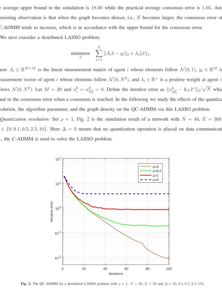
N which is equal to the consensus error when a consensus is reached. In the following we study the effects of the quantization resolution, the algorithm parameter, and the graph density on the QC-ADMM via this LASSO problem.

Quantization resolution: Set ρ = 1. Fig. 2 is the simulation result of a network with N = 40, E = 300 and

∆ ∈ {0,0.1,0.5,2.5,10}. Here ∆ = 0 means that no quantization operation is placed on data communications, i.e., the C-ADMM is used to solve the LASSO problem.

Iterations 0 20 40 60 80 100 Iterative error 10-2 10-1 100 101 102 ∆=0 ∆=0.2 ∆=1 ∆=5

Fig. 2: The QC-ADMM for a distributed LASSO problem withρ= 1,N= 40,E= 40and∆∈ {0,0.1,0.5,2.5,10}.

We observe that the consensus error becomes larger as ∆ increases. This is not surprising as the higher the quantization resolution is, the more information is lost at each update, thus resulting in a higher consensus error. Meanwhile, the convergence time decreases when ∆ increases, which can be seen from the upper bound on the

number of iterations that guarantees the convergence of the QC-ADMM; that is, Ωin (41) decreases as∆becomes larger. On the other hand, a larger∆indicates a sparser quantization lattice which makes it easier for the QC-ADMM reach a convergence point.

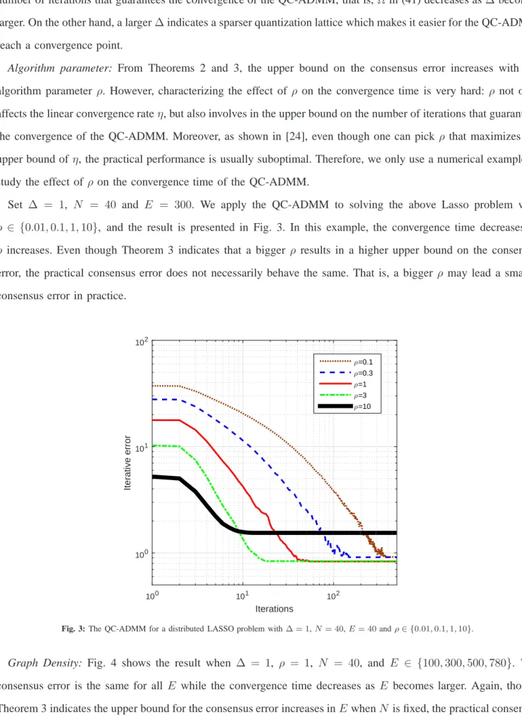
Algorithm parameter: From Theorems 2 and 3, the upper bound on the consensus error increases with the

algorithm parameter ρ. However, characterizing the effect of ρ on the convergence time is very hard: ρ not only affects the linear convergence rateη, but also involves in the upper bound on the number of iterations that guarantees the convergence of the QC-ADMM. Moreover, as shown in [24], even though one can pick ρ that maximizes the upper bound of η, the practical performance is usually suboptimal. Therefore, we only use a numerical example to study the effect of ρ on the convergence time of the QC-ADMM.

Set ∆ = 1, N = 40 and E = 300. We apply the QC-ADMM to solving the above Lasso problem with

ρ _{∈ {}0.01,0.1,1,10_}, and the result is presented in Fig. 3. In this example, the convergence time decreases as

ρ increases. Even though Theorem 3 indicates that a bigger ρ results in a higher upper bound on the consensus error, the practical consensus error does not necessarily behave the same. That is, a bigger ρ may lead a smaller consensus error in practice.

Iterations 100 101 102 Iterative error 100 101 102 ρ=0.1 ρ=0.3 ρ=1 ρ=3 ρ=10

Fig. 3: The QC-ADMM for a distributed LASSO problem with∆ = 1,N= 40,E= 40andρ∈ {0.01,0.1,1,10}.

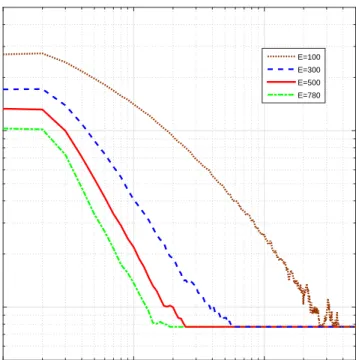
Graph Density: Fig. 4 shows the result when ∆ = 1, ρ = 1, N = 40, and E _{∈ {}100,300,500,780_}. The consensus error is the same for all E while the convergence time decreases as E becomes larger. Again, though Theorem 3 indicates the upper bound for the consensus error increases inEwhenN is fixed, the practical consensus

error need not necessarily perform the sam and can be much smaller. WhenE increases withN fixed, the average degree of the graph also increases. Then on the average, an agent can communicate with more agents at each update, thus resulting in a fast convergence.

Iterations 100 101 102 Iterative error 100 101 E=100 E=300 E=500 E=780

Fig. 4: The QC-ADMM for a distributed LASSO problem with∆ = 1,ρ= 1,N= 40,E=∈ {100,300,500,780}.

V. CONCLUSION

This paper proposes an efficient algorithm, the QC-ADMM, for multi-agent distributed optimization under the quantized communication constraint. We show that this algorithm can be derived from the standard ADMM by adding a quantization operation on xk immediately after the x-update together with proper initializations. While existing quantized ADMM approaches only apply to quadratic local objectives, the QC-ADMM can deal with more general objective functions, possibly non-smooth. Specifically, the QC-ADMM converges to a consensus within finite iterations under certain convexity conditions, which further enables us to derive a tight upper bound on the consensus error. Moreover, the proof idea provides a framework for convergence proof of a class of inexact updated algorithms.

Our approach also motivates future research directions:

1) We assume the quantized data communication between agents to be perfect in this paper. In practice, channel impairment may lead to imperfect transmissions. Moreover, the links between agents may fail and the topology of the network may vary. It is thus interesting to investigate how our algorithm performs in such settings.

2) Recent work of [30], [31] proposes computationally efficient distributed ADMM algorithms that have linear convergence rates under certain conditions. We expect that the idea of this paper can also lead to quantized ADMM algorithms with significantly reduced computational complexity.

REFERENCES

[1] D. Bertsekas and J. Tsitsiklis, Parallel and Distributed Computation: Numerical Methods, 2nd ed. Nashua, NH, USA: Athena Scientific, 1997.

[2] G. Giannakis, Q. Ling, G, Mateos, I. Schizas, and H. Zhu, “Decentralized learning for wireless communications and networking,” ArXiv, 2015.

[3] W. Ren, R. W. Beard, and E. M. Atkins, “Information consensus in multivehicle cooperative control,” IEEE Contr. Syst. Mag., vol. 27, no. 2, pp. 71–82, Apr. 2007.

[4] N. Lynch, Distributed Algorithms. San Francisco, CA: Morgan Kaufmann, 1996.

[5] L. Xiao, S. Boyd, and S. Lall, “A scheme for robust distributed sensor fusion based on average consensus,” Proc. Int. Conf. Information Processing in Sensor Networks, Los Angeles, CA, Apr. 2005.

[6] R. Bekkerman, M. Bilenko, and J. Langford, Scaling Up Machine Learning: Parallel and Distributed Approaches. Cambridge University Press, 2012.

[7] G. R. Andrews, Foundations of Multithreaded, Parallel, and Distributed Programming. Addison-Wesley, 2007.

[8] H. Zhu, G. B. Giannakis, and A. Cano, “Distributed in-network channel decoding,” IEEE Trans. Signal Process., vol. 57, no. 10, pp. 3970–3983, 2009.

[9] S. Zhu and B. Chen, “Quantized consensus by the ADMM: probabilistic versus deterministic quantizers,” ArXiv, 2015.

[10] G. Mateos, J. Bazerque, and G. Giannakis, “Distributed sparse linear regression,” IEEE Trans. Signal Process., vol. 58, no. 10, pp. 1856–1871, 2009.

[11] Q. Ling and Z. Tian, “Decentralized sparse signal recovery for compressive sleeping wireless sensor networks,” IEEE Trans. Signal Process., vol. 58, no. 7, pp. 3816–3827, 2010.

[12] J. Bazerque and G. Giannakis, “Distributed spectrum sensing for cognitive radio networks by exploiting sparsity,” IEEE Trans. Signal Process., vol. 58, no. 3, pp. 1847–1862, 2010.

[13] L. Gan, U. Topcu, and S. Low, “Optimal decentralized protocol for electric vehicle charging,” IEEE Trans. Power Syst., vol. 28, no. 2, pp. 940–951, 2013.

[14] M. Rabbat and R. Nowark, “Quantized incremental algorithms for distributed optimization,” IEEE J. Sel. Areas Commun., vol. 23, no. 4, pp. 798–808, 2006.

[15] D. Yuan, S. Xu, H. Zhao, and L. Rong, “Distributed dual averaging method for multi-agent optimization with quantized communication,” Syst. Control Lett., vol. 61, no. 11, pp. 1043–1061, 2012.

[16] A. Nedi´c, A. Olshevsky, A. Ozdaglar, and J. N. Tsitsiklis, “Distributed subgradient methods and quantization effects,” in Proc. IEEE Conf. on Decision and Control, Cancun, Mexico, 2008.

[17] A. Nedi´c and D. P. Bertsekas, “Incremental subgradient methods for nondifferentiable optimization,” SIAM J. Optim., vol. 56, no. 1, pp. 109–138, 2001.

[18] J. Duchi, A. Agarwal, and M. Wainwright, “Dual averaging for distributed optimization: convergence analysis and network scaling,” IEEE Trans. Autom. Control, vol. 57, no.3, pp. 592-606, 2012.

[19] A. Nedi´c and A. Ozdaglar, “Distributed subgradient methods for multi-agent optimization,” IEEE Trans. Autom. Control, vol. 54, no. 1, pp. 48–61, 2009.