Semi-supervised Hyperspectral Band Selection
via Spectral-spatial Hypergraph Model
Xiao Bai, Zhouxiao Guo, Yanyang Wang, Zhihong Zhang, Jun Zhou
Abstract—Band selection is an essential step towards ef-fective and efficient hyperspectral image classification. Tradi-tional supervised band selection methods are often hindered by the problem of lacking enough training samples. To address this problem, we propose a semi-supervised band selection method that allows contribution from both labelled and unlabelled hyperspectral pixels. This method first builds a hypergraph model from all hyperspectral samples in or-der to measure the similarity among pixels. We show that hypergraph can captures relationship among pixels in both spectral and spatial domain. In the second step, a semi-supervised learning method is introduced to propagate class labels to unlabelled samples. Then a linear regression model with group sparsity constraint is used for band selection. Finally, hyperspectral pixels with selected bands are used to train a support vector machine classifier. The proposed method is tested on three benchmark datasets. Experimental results demonstrate its advantages over several other band selection methods.
Index Terms—Hyperspectral imaging, Band selection, Hy-pergraph, Image classification.
I. INTRODUCTION
Hyperspectral imagery has been used in a variety of re-mote sensing applications. It contains hundreds of spectral bands with nanoscale spectral resolution, which provides valuable information for target detection and classification. However, such abundant wavelength indexed bands also contain redundant or correlated information which influence the effectiveness and efficiency of data modelling [1]. An intuitive way of solving this problem is selecting a subset of bands from the original data [2].
Band selection methods can be categorized as supervised or unsupervised. Supervised learning methods use labelled data to determine the importance of bands. Class labels are often generated by manual annotation or ground survey. The learning outcome can be a searching strategy, or a class separability criterion. For instance, Yang et al. [3] proposed a sequential forward selection (SFS) searching
This research is supported under China NSFC Projects (No.61105022) and Australian Research Council’s DECRA Projects funding scheme (project ID DE120102948)
Xiao Bai and Zhouxiao Guo are with the School of Computer Sci-ence and Engineer, Beihang University, Beijing 100191, China. (e-mail: [email protected].)
Yanyang Wang is with the School of Aeronautic Science and Engineering, Beihang University, Beijing 100191, China. (e-mail: [email protected].)
Zhihong Zhang is with the Software School of Xiamen University, Siming District, China
Jun Zhou is with the School of Information and Communication Technology, Griffith University, Nathan, Queensland 4111, Australia.
strategy for band selection. In [4], Rick Archibald et al introduced an embedded feature selection algorithm that is tailored to operate with support vector machines. In [5], bands were selected according to transformed divergence measure and the maximum likelihood accuracy on the test data.
Unsupervised methods, on the contrary, do not need to learn a predictive model from training data. Classic unsupervised methods, for example, principal component analysis [6] and affinity propagation [7], often use a priori knowledge of the scene to measure the statistical depen-dence between bands in order to evaluate the contribution of each band in the classification. Some methods, such as linear prediction [8] and geometrical feature selection [9], search for distinctive spectral signatures based on different considerations of band properties. Ghamary Asl et al. [10] proposed a method to select distinct and informative bands in a prototype space which is constructed by clustering of raw image data. Bands are selected based on either their orthogonal distance to the diagonal of the prototype space or their angle distance that is related to the correlation between neighboring bands. In unsupervised band selection, searching algorithms are required in most cases [11], which can be speeded up via parallel computing techniques [12]. The evaluation of the effectiveness of band selection ap-proaches can be done at either the band level [13] or the whole data cube level [14].
Despite their advantages in implementation, unsuper-vised methods can not match the classification accuracy of the supervised methods. As a consequence, semi-supervised band selection methods, which combine the advantages of both supervised and unsupervised methods, have attracted the attention from the research community. Bai et al. [15] proposed a semi-supervised learning method that estimates the vectors of mean values and covariance matrices for each class under the assumption of a Gaussian mixture model. Chen et al combined Fisher’s criteria and graph Laplacian to explore both labeled and unlabeled samples simultaneously [16]. Moreover, mutual information has also been used as a measurement criterion via graph regulation term [17]. These methods have shown their effectiveness when the amount of labelled data is insufficient.
Recently, hypergraph based methods have been proposed for pattern recognition [18] and image processing [19]. In [20] and [21], hypergraph construction methods have been introduced for hyperspectral band selection. These methods use spectral mutual information to build a hyper-graph which is used for label propagation. However, both
methods have not considered spatial information between pixels in the hyperspectral imagery. In this paper, we propose a semi-supervised band selection method based on hypergraph model which combines both spectral and spatial properties of data. Based on pairwise sample similarity generated from traditional undirected graph, this method first constructs a hypergraph model of all samples, both labeled and unlabeled, in a hyperspectral image. Each vertex of the hypergraph is a pixel, and edges between vertices show the similarity between pixels in both spectral feature space and spatial space. In this way, a matrix can be calculated on the hyperspectral image, which captures mul-tiple relationships between data samples. In the second step, a projection matrix is learned in a semi-supervised manner, which propagates the class information from labeled data to unlabeled data. Band selection is implemented by solving a sparse group constrained linear regression problem on the whole hyperspectral image. This enables selection of not only individual band, but also groups of bands that are useful for image classification. This method is assessed via experiments on three hyperspectral datasets. The results show that joint spectral-spatial hypergraph construction in affinity matrix calculation and the sparse group constraints in band selection can effectively improve the classification performance.
The contributions of this paper lies in four aspects. Firstly, we present a hypergraph model that generalizes the traditional graph model for band selection. We show that hypergraph is a better approach to characterize the similar-ity between hyperspectral pixels. This lead to more reliable label propagation in semi-supervised band selection. Sec-ondly, we introduce spectral and spatial information into hyperedge calculation. Such joint spectral spatial analysis has demonstrated significant advantages over the traditional spectral only analysis. Thirdly, a sparse group constrained linear regression model is used for band selection. This model selects not only individual bands, but also a group of bands that are discriminative for image classification. Fourthly, we perform comprehensive experiments to com-pare the proposed method with several alterative methods in the literature. In-depth analysis on key steps is provided, which allows better understanding of the proposed method. The rest of this paper is organized as follows. Section II introduces the hypergraph construction and sample simi-larity calculation method. Section III introduces the label propagation and sparse group constrained linear regres-sion methods for band selection. Section IV describes the datasets used in the experiments and the image classifica-tion results.
II. HYPERGRAPHMODEL
In this section, we first introduce traditional un-directed graph representation. Then we propose a spectral-spatial hypergraph model to calculate the similarities among hy-perspectral image pixels. Hypergraph is a special graph representation where each edge can connect more than two vertices. Compared with traditional un-directed graph,
hypergraph can better characterize the complex relationship inside the hyperspectral data.
A. Graph on Hyperspectral Samples
Given a hyperspectral image X = [x1, . . . ,xN] ∈
RN×M wherexi represents a vector of spectral responses at a pixel or sample location in a hyperspectral image. N
is the number of pixels and M is the number of spectral bands. LetG= (V,E,W)be a weighted un-directed graph
defined onX.Vis a set of vertices consist ofN samples in X, andEare the edges connecting vertices.Wis a matrix
whose entries correspond to the weights of edges, each of which characterizing the similarity between two vertices connected by an edge.
When constructed from a hyperspectral image, the edge weight matrixWof the graph can be defined as follows:
Wij=e−||xi−xj||
2/σ
(1) whereσis a scalar parameter, which is the variance of the average distance between samples. In this definition,xiand
xj can be either labeled or unlabeled samples inX. If two samples are close to each other, i.e., the Euclidean distance between two spectral vectors is small, a large edge weight is generated. Otherwise, a small edge weight is obtained.
B. Hypergraph Model
The weights of graph defined above only describe the relationship between two samples in a hyperspectral im-agery. In many cases, the support on similarity computation comes from more than two samples. For example, each pixel in a hyperspectral image may be grouped with its neighboring pixels, or with several very similar pixels in the spectral feature space. Then the similarity calculation between arbitrary pixel pair can be converted to calculating the similarity between two groups of pixels.
To facilitate such group-wise similarity calculation, we introduce the concept of hypergraph. A hypergraph is a gen-eralization of a graph in which an edge can connect more than two vertices. Therefore, it enables better description on the complex relationship between pixels [22].
Let a hypergraph G˜ be defined as G˜ = (V,E˜,W˜ ).
V = {x1, . . . ,xN} is a set of vertices with the same
definition as in the traditional un-directed graph,E˜ is a set
of non-empty subsets ofV called hyperedges. W˜ is a set
of weight functions which correspond to each hyperedge. A hyperedge can connect an arbitrary number of vertices. In this paper, we only consider K-uniform hypergraph in which every hyperedge connects the same number of K
vertices, i.e., a hyperedgeE˜i={xi1, . . . ,xiK}.K-uniform
is a widely used option of constructing a hypergraph. It is desirable that each hyperedge contains a set of vertices that have some common properties [23]. Given a vertex
xi∈X, the selection ofKvertices to constructE˜iis based on the edge weight matrixWdefined in equation (1). Let
xiK =xi, only K−1 vertices with top Wij values, i.e.,
those pixels closest toxi in the spectral feature space, are selected to form {xi1, . . . ,xiK−1}. Therefore, the number
of hyperedges is the same as the number of vertices. There are two reasons to use top K−1vertices to construct the hyperedges of a hypergraph. First, topK−1similar vertices share the highest common spectral property, compared to the rest of vertices. Second, using topK−1vertices saves the computation time than using all vertices.
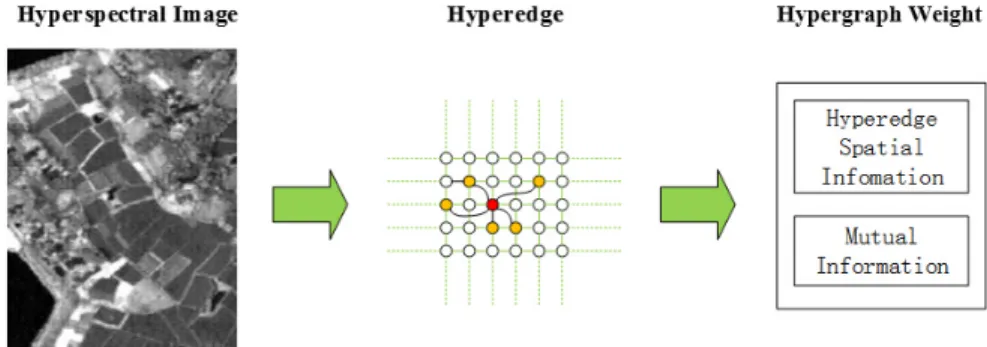
Compared with the tradition graph definition, the hyper-edge in a hypergraph can connect more than two vertices. Therefore, the definition of the weight for hyperedge should consider the relationship among multiple vertices connected by the edge. In this paper, the weight W˜ (i)of hyperedge
˜
Ei consists of two terms that incorporate both spatial and spectral information in the hypergraph construction. The first term is W˜ s which is calculated after considering the spatial relationship between pixels, and the second term is mutual information W˜ min the spectral feature space.
Formally, the weight of a hyperedge can be defined as ˜
W(i) =tW˜ s(i) + (1−t) ˜Wm(i) (2) wheretis a parameter in[0,1], which determines the trade-off between spectral and spatial information of the pixels used to construct a hyperedge. Analysis on howtinfluences the band selection and image classification performance is given in Section IV-A. In practice, the optimal value of t
can be determined by cross validation.
The spatial informationW˜ s(i)of hyperedgeE˜iis com-puted as follows ˜ Ws(i) = X {a,b}⊂{i1,...,iK} 2wa,b K∗(K−1) (3) where wa,b=e−||ca−cb|| 2/σ (4) In the above equation,ca andcb are the pixel coordinates of two samples indexed by a and b in the hyperedge,
||ca−cb|| is the spatial distance between these two sam-ples, andσ is a scale parameter controlling the decay rate of the distance. The definition ofW˜ s(i)reflects the overall spatial distance among vertices in a hyperedge. In cases when two pixels have similar spectral information but are distant from each other, according to Equation (4), a small weight wa,b will be generated. Since the spatial informa-tion W˜ s(i) is summed over all weights as presented in Equation (3), this small weight does not generate significant impact to the final calculation.
The second component in Equation (2) is the mutual informationW˜m(i)of hyperspectral pixels, which is com-puted as follows
˜
Wm(i) =K Ixi1,...,xiK
H(xi1) +. . .+H(xiK)
(5)
where Ixi1,...,xiK is the multivariate mutual information
among hyperspectral pixels indexed byxi1, . . . ,xiK. It can
be calculated as follows [24] Ixi1,...,xiK = K X k=1 (−1)k−1 X Xs⊂ {xi1, . . . ,xiK} |Xs|=k H(X) (6)
In Equation (6), Xs is a subset of {xi1, . . . ,xiK}, and H(Xs) represents the Shannon entropy of a discrete ran-dom variable with possible values and probability mass function. If Xs is in the form of single variable xik =
[xik1, . . . ,xikM]
T, where M is the total number of hyper-spectral bands, the entropy can be explicitly calculated as follows H(xik) = M X m=1 P(xikm)I(xikm) =− M X m=1 P(xikm)log2(xikm) (7)
When there are more than two variables, this expands to
H(Xs= [xi1, . . . ,xid]) =−X xi1 . . .X xid P(xi1, . . . ,xid) log2[P(xi1, . . . ,xid)] (8) wheredis the number of vertices in random variable Xs.
P(xi1, . . . ,xid)is the probability ofxi1, . . . ,xidoccurring
together. P(xi1, . . . ,xid) log2[P(xi1, . . . ,xid)] is defined
to be 0 ifP(xi1, . . . ,xid) = 0.
It is clear that the greater the value ofIxi1,...,xiK is, the
more relevant theK vertices are.
Algorithm 1: Hypergraph construction algorithm Data: DatasetX= [x1, ..,xN]∈RN×M with each
row being a spectral feature vector in the hyperspectral imagery.
Compute similarity matrix:Wij=e−||xi−xj||
2/σ
; fori= 1 toN do
1. Arrange Wij in descending order; 2. Select the firstK−1 vertices andxi to construct a hyperedgeE˜i={xi1, . . . ,xiK};
3. CalculateW˜ s(i)using Equation (3); 4. CalculateW˜ m(i)using Equation (5); 5. CalculateW˜ (i) =tW˜ s(i) + (1−t) ˜Wm(i); end
The hypergraph construction method is summarized in Fig. 1 and Algorithm 1. There is no widely accepted method to handle the operation of hypergraph weight matrix. In our method, we convert the hypergraph weight matrix into an affinity matrix M ∈ RN×N in order to facilitate the
computation in the later steps. Weights of all hyperedges containingxa andxb are added up to generate the weight of Ma,b. Therefore,Ma,b is computed as
Ma,b= X i s.t. xa,xb∈E˜i ˜ W(i) (9)
To show how the entries of the affinity matrix are calcu-lated, we give the following example. Letx1andx2be two
pixels whose affinity is to be calculated. AssumeK = 4, i.e., a hyperedge contains four vertices. If three hyperedges
Fig. 1. Construction of hypergraph.
contain both x1 and x2, i.e., E˜1 = {x1,x2,x3,x4},
˜
E2 = {x1,x2,x4,x5}, E˜3 = {x1,x2,x5,x7}, E˜4 =
{x3,x4,x5,x7}, thenM1,2= ˜W1+ ˜W2+ ˜W3.
III. BANDSELECTION ANDIMAGECLASSIFICATION In this section, we move on to the band selection method. After the hypergraph has been transformed into an affinity matrix, our goal is to convert the high dimensional dataX∈
RN×M to low dimensional dataY∈RN×D (D << M),
whereM andDare the number of bands before and after band selection, respectively. This dimensionality reduction problem can be modeled as a special subspace learning task, where the projection matrix is constrained to be a selection matrix S, such that Y = XS. To utilize both labeled and unlabeled data, a semi-supervised learning method, which consists of label propagation and selection matrix learning, is introduced. Finally, all bands are sorted based on sparse matrix S, and the top bands are selected as the final outcome. In summary, this stage has four steps, which include label propagation, sparse matrixSestimation, band selection, and image classification.
A. Label Propagation
Given a dataset of pixels X = [x1, . . . ,xl, . . . ,xN] ∈
RN×M withl labeled samples and u =N −l unlabeled
samples, the goal of label propagation is to estimate which classes the unlabeled samples belong to.
We adopted the label propagation method by Nie et al. [25], which not only achieves the goal of semi-supervised learning, but also discovers the latent novel class in the data. Define an initial label matrix L∈RN×(C+1),
whereCis the number of classes of the data. An additional class labelC+ 1is added to record the outliers. The initial value of label matrix is defined as follows:
Li,j=
1 if xi is labeled as li=j or j=C+ 1
0 otherwise
(10) Let F ∈ RN×(C+1) denotes the set of classification
function defined onX. SinceFworks on both labelled and unlabelled data, it can be considered as a label propagation matrix, i.e.,Fij represents the probability that samplesi be-long to classj. In every propagation step, each data absorbs
a fraction of the label information from its neighborhood and also retains some label information of its initial state. To propagate labels, we define a matrixPasP=D−1M,
where D is a diagonal matrix with Dii =PjMi,j, and
M is the affinity matrix calculated from hypergraph. This is equivalent to the normalization process for matrix M. Then the label ofxi at timet+ 1can be updated from its previous estimationF(t)
F(t+ 1) =λPF(t) + (1−λ)L. (11) whereλis a parameter in[0,1]. The above steps iterate until convergence. LetF∗denotes the limit of the sequenceF(t), the final estimation functionF∗ can be computed directly using an analytical solution without iterations
F∗= lim
t→∞F(t) = (1−λ)(I−λP)
−1L (12)
whereIis an identity matrix. Hence, we can useF∗as the classification function so that the labels of hyperspectral samples can be predicted in one step.
B. Sparse MatrixS
After the label propagation matrix F∗ is calculated, the next step is to learn the sparse selection matrixS. Here we build a linear classifiery=STx+bwherexis a sample in the hyperspectral imagery andbis a bias term. Ifyis close togj wheregj = [0, . . . ,0,1,0, . . . ,0]T which means the
jth element in gj is 1 , x will be classified into class j. Assuming that the result of classification from the linear classifier equals the above semi-supervised learning matrix
F∗, we can define a regression function as follows
argmin S,b N X i=1 C X j=1 F∗i,j||STxi+b−tj||2 (13) In order to find an optimal subset of bands, we adopt the Lasso method [26] which is an L1-constrained fitting
solution for statistics and data mining. It minimizes the residual sum of squares subject to the sum of the absolute value of the coefficients being less than a constant. This forces many entries of S to be zeros.
Considering that neighboring spectral bands may be highly correlated, we also group the neighboring bands and
solve the band selection problem using the group LASSO method [27]. To do so, we uniformly divide the spectral bands into R groups. Then the group Lasso imposes a combination of L1 and L2 penalties on the regression
coefficients. Therefore, the loss function is designed to eliminate the impact of the outlier as well as to achieve the minimal reconstruction error, while encouraging only some bands in the useful band groups be selected.
The regression function can be written as
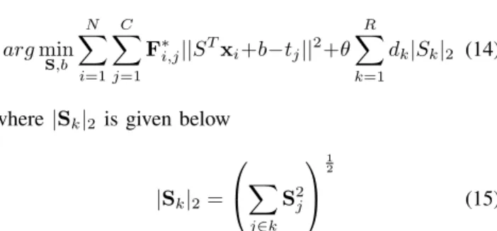
argmin S,b N X i=1 C X j=1 F∗i,j||STxi+b−tj||2+θ R X k=1 dk|Sk|2 (14)
where|Sk|2 is given below
|Sk|2= X j∈k S2j 1 2 (15)
whereF∗i,jis the element from the label propagation matrix in Equation (12) and θ is a parameter in[0,1].dk is a set of strictly positive fixed weights. Therefore, the sum over
R groups is essentially the L1 penalty term of the group
sparsity.
C. Band selection
Note the goal of band selection is to selectDbands from a total of M band candidates. Here, we use band score to evaluate every band from the selection matrixS, which is defined as
bandscore(j) = max
k |Sj,k| (16) where j is the band index, Sj,k is the jth row of Sk. After getting scores of all the bands, we sort the bands in descending order and select the top D bands as the outcome.
D. Image Classification
Finally, we perform image classification based on the se-lected bands which are the same for all samples. A support vector machine (SVM) classifier is applied to the selected bands of each sample to be classified in the hyperspectral remote sensing images. The classification process is carried out for each sample individually. SVM is used here because of its good performance in the nonlinear separable problem and small training sample sets. In this step, the Gaussian radial basis function (RBF) [28] is chosen as the kernel function, which is defined as
KF(xi,x) =exp(−γ||xi−x||) (17)
whereγ is a parameter inversely proportional to the width of the Gaussian kernel. xandxi are samples and support vectors whose dimension is D.
IV. EXPERIMENTS
Having presented our method in the previous sections, we now turn our attention to demonstrating its utility for classification. Three real-world hyperspectral image datasets have been used for experiments. They are APHI dataset, Indian Pines dataset, and Washington DC Mall dataset. We compared the overall classification accuracy of our method with those from several alternative methods in the literature. These methods include band selection methods based on semi-supervised learning, unsupervised learning, and uniform sampling, as follows
• Uniform sampling (Uniform) which selects bands uni-formly.
• Maximum-Variance PCA (MVPCA) [6] which ranks bands based on their importance and their correlation with other bands.
• Mutual Information-based Information Divergence (ID) [2] which selects bands based on mutual infor-mation.
• FCGL [29] which is a semi-supervised algorithm that combines Fisher’s criteria and graph Laplacian to explore both labeled and unlabeled samples at the same time.
In the experiments, the values of some key parameters were determined by cross validation on the training data. In particular, K = 9 in Equation (9), λ = 0.92 in Equation (12), and θ= 0.25 in Equation (14). The kernel parameter γ in Equation (17) was obtained by cross-validation on a subset of the training samples [30]. In the group LASSO solution for the regression model in Equation (13), each group consisted of 20 neighboring bands.
A. APHI Dataset
The APHI (Airborne Push hyperspectral Imager) data is 210×150×64 in size and covers 455nm to 805nm in spec-tral range. It was acquired from an altitude of approximately 20km with 18m in spatial resolution. The number of bands in the APHI dataset is 64. Fig. 2 displays the 26th band of APHI imagery. The ground truth of APHI data is shown in Fig. 3. The land cover types of APHI dataset are paddy, bamboo, tea, pachyrhizus, caraway and water, respectively.
Fig. 3. Ground truth of APHI dataset.
The performance of band selection is evaluated by the classification accuracy. To this end, both labeled and un-labeled samples were randomly selected to train a semi-supervised classifier. Labels of samples were firstly prop-agated to unlabeled samples, which were then used to train an SVM classifier. In the APHI dataset, we randomly selected 340 labeled samples and 2410 unlabeled samples for label propagation and classifier learning and testing. Table I displays the detailed number of samples for each class during the label propagation and classification step.
TABLE I
NUMBER OF LABELED AND UNLABELED SAMPLES FROMAPHI
DATASET USED IN THE EXPERIMENTS. Class Labeled samples Unlabeled samples
Paddy 100 800 Bamboo 50 280 Tea 50 280 Pachyrhizus 30 250 Caraway 50 200 Water 60 800 Total 340 2410
In the label propagation step, for all 6 land-cover classes, 12% samples of each class were randomly selected as the labeled samples and the remaining ones were used as the unlabeled samples. Both labeled and unlabeled samples were randomly chosen from the dataset for five times. The same training and testing samples were also used in the classification step.
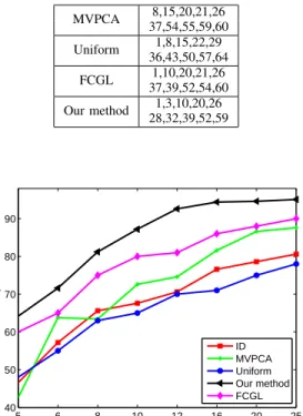
Fig. 4 presents the classification results compared with other band selection methods. To investigate the impact of different number of selected bands on the classification accuracy, we varied this number from 5 to 25 and compared the accuracy of different methods. It can be seen that our method has outperformed all alternative methods, followed by FCGL and MVPCA. Uniform sampling method has delivered the lowest classification accuracy. This shows the effectiveness of band selection from our method. When the number of bands increases, the classification accuracy also increases for each method. The proposed hypergraph based method is close to convergence when the band number
reaches 16. Table II lists the selected bands by four methods when the number of bands is set to 10.
TABLE II
SELECTED BANDS FROMAPHIDATASET BY DIFFERENT METHODS. MVPCA 8,15,20,21,26 37,54,55,59,60 Uniform 1,8,15,22,29 36,43,50,57,64 FCGL 1,10,20,21,26 37,39,52,54,60 Our method 1,3,10,20,26 28,32,39,52,59 5 6 8 10 12 16 20 25 40 50 60 70 80 90 Number of bands Accuracy rate ID MVPCA Uniform Our method FCGL
Fig. 4. Classification accuracies on the APHI dataset by different methods.
Parameter t in Equation (2) controls the contribution from the spatial and spectral information in the hyper-edge weight calculation. To evaluate such contribution, we calculated the classification accuracies on the APHI data with changing t values, as shown in Fig. 5. This figure shows that the best classification performance is reached when t = 0.425. It suggests that both spatial and spectral information are important in the hypergraph construction step. This is reasonable because spatial and spectral relationships are two key relationships between hyperspectral pixels.
B. Indian Pines AVIRIS Dataset
Indian Pines AVIRIS dataset was collected by Air-borne Visible/Infrared Imaging Spectrometer. We consid-ered 9 land-cover classes which are corn-notill, corn-min, grass/pasture, grass/tree, hay-windrowed, soybeans-min, soybeans-notill, soybeans-clean, and woods. A pseudo-color image constructed by bands 26, 100, and 47 is shown in Fig. 6 whose ground truth is displayed in Fig. 7. After removing water absorption and noisy bands, 200 bands were used for the experiments.
On the Indian Pines dataset, we randomly selected 1081 samples as the training data and 5407 samples as the testing data. This process repeated 10 times to generate ten different random splits of datasets. The number of training and test samples in each class are shown in Table III.
0 0.2 0.4 0.6 0.8 1 78 80 82 84 86 88 90 92 94 Paremeter t Accuracy rate
Fig. 5. Classification accuracy on the APHI dataset with different contri-bution from spectral and spatial information in hypergraph construction.
Fig. 6. Pseudo-color image constructed from bands 26, 100 and 47 in the Indian Pines dataset.
Fig. 7. Ground truth of the Indian pines dataset. TABLE III
NUMBER OF TRAINING AND TESTING SAMPLES FOR EACH CLASS IN THEINDIANPINES DATASET.
Class training samples testing samples
Corn-notill 100 900 Corn-min 111 556 Grass/Pasture 140 280 Grass/Tree 100 250 Hay-windrowed 80 280 Soybeans-notill 100 800 Soybeans-min 300 1500 Soybeans-clean 50 410 Woods 100 800 Total 1081 5407
Table IV lists the indices of selected bands when the number of bands is set to 10. The table shows that some bands are unanimously selected by different band selection
methods, for example, band 11 in the Indian Pines data, which suggests that these bands are the most informative bands for hyperspectral classification.
TABLE IV
SELECTED BANDS FROM THEINDIANPINES DATASET BY DIFFERENT METHODS. MVPCA 1,11,26,32,35 97,37,184,185,186 Uniform 101,121,141,161,1811,21,41,61,81 FCGL 4,11,15,21,29 79,82,94,128,186 Our method 61,76,90,128,1342,7,11,25,32
Fig. 8 shows the change of accuracies when different number of bands are selected. Similarly, the best result is produced when the number of selected band exceeds 20. It can be seen that the proposed method has consistently outperformed MVPCA, Uniform, FCGL and ID methods. This figure also shows that when selecting more than 20 bands, the gain on the accuracy is not as significant as the gain on smaller number of bands. This suggests that 20 bands can be considered as the preferred number of bands to be selected. 5 8 10 15 20 30 40 50 40 45 50 55 60 65 70 75 80 85 Number of bands Accuracy rate ID MVPCA Uniform Our method FCGL
Fig. 8. Classification results on the Indian Pines dataset when the number of selected bands varies.
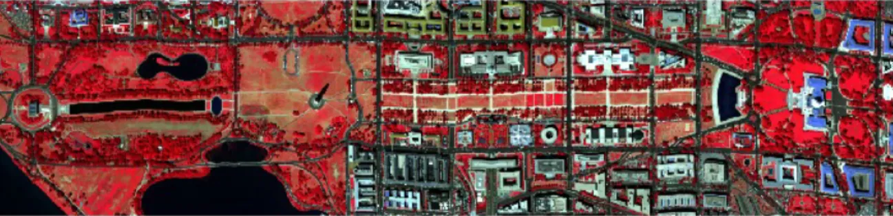
C. Washington DC Mall dataset
We also performed experiments on the airborne hyper-spectral HYDICE data captured at the Washington DC mall. It has 210 spectral bands from 400nm to 2500nm, and 1208 scan lines with 307 pixels in each scan line. The totally available classes are nine. Fig. 9 displays a pseudo-color image of the dataset and Fig. 10 shows the region we selected for experiments and the ground truth labels. In the experiments, we used 6 classes which are road, grass, shadow, trail, tree, and roof, respectively. The numbers of labeled samples and unlabeled samples in each class are shown in Table V. These were used to train the band selection methods and the SVM classifiers.
Fig. 11 shows the classification accuracy of each band selection method. Obviously, compared with other band
Fig. 9. Pseudo-color image of the HYDICE data on Washington DC Mall.
Fig. 10. Selected region and ground truth of the Washington DC Mall dataset.
TABLE V
NUMBER OF LABELED AND UNLABELED SAMPLES IN THE
WASHINGTONDC MALL DATASET. Class Labeled samples Unlabeled samples
Road 50 200 Grass 100 900 Shadow 20 100 Trail 100 800 Tree 80 360 Roof 100 400 Total 450 2760 TABLE VI
SELECTED BANDS FROM THEWASHINGTONDC MALL DATASET BY DIFFERENT METHODS. MVPCA 3,9,13,46,64 89,150,152,182,184 Uniform 21,41,61,81,101 121,141,161,181,201 FCGL 8,9,36,88,89 151,152,180,182,184 Our method 3,9,39,64,88 89,152,180,182,184
selection methods, which include both semi-supervised and unsupervised band selection options, our method can better predict the class labels of samples in the hyperspectral imagery. We can also observe that, when the number of selected band is the same, our method yields the best results in most of the cases. Note that the accuracy increases with more bands being selected. Our method converges when 30 bands are selected. The top 10 selected bands on this dataset are shown in Table VI.
5 8 10 15 20 30 40 50 40 45 50 55 60 65 70 75 80 85 Number of bands Accuracy rate ID MVPCA Uniform FCGL Our method
Fig. 11. Classification accuracy on the Washington DC Mall dataset.
D. Efficiency comparison
Now we illustrate the computational costs of our method and other band selection methods. The codes for all methods were run on a laptop with Intel(R) Core(TM) i5 CPU. Table VII reports the time cost of each method on three benchmark datasets. From the table, we can see that ID is the fastest method and all other methods are much more time-consuming. This is because the ID method is an unsupervised method without spending time on label propagation. Our method is superior than the semi-supervised band selection method FCGL and unsemi-supervised method MVPCA on both Indian Pines and APHI datasets. However, it is slower than others on the Washington DC Mall dataset. This is mainly because the construction of
3 4 5 6 7 8 9 12 20 30 0.75 0.8 0.85 0.9 0.95 1 Numbers of bands
Correlation of Selected bands
ID MVPCA FCGL Our method 3 4 5 6 7 8 9 10 11 12 13 14 15 20 30 40 50 0.75 0.8 0.85 0.9 0.95 1 Numbers of bands
Correlation of Selected bands
ID MVPCA FCGL Our method 3 4 5 6 7 8 20 30 40 50 0.75 0.8 0.85 0.9 0.95 1 Numbers of bands
Correlation of Selected bands
ID MVPCA FCGL Our method
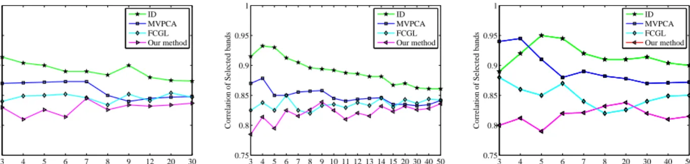
Fig. 12. Correlation measures between the selected bands produced by ID, MVPCA, FCGL, and our method on three datasets. From left to right are the results on the APHI, the Indian Pines, and the Washington DC Mall datasets.
hypergraph requires larger number of testing and training samplings operations on the Washington DC Mall dataset than on the other two datasets.
TABLE VII
COMPUTATIONAL COST OF DIFFERENT BAND SELECTION METHODS
Time cost ID MVPCA FCGL Our method Indian Pines 10s 3m10s 2m4s 2m2s
APHI 7s 2m6s 2m 1m25s
Washington DC Mall 11s 3m4s 4m 5m25s
E. Group Sparsity
We conducted an experiment to compare the basic spar-sity and group sparspar-sity methods on classification accuracy. For the group sparsity option, we uniformly divided the bands into groups of 20 neighboring bands and calculate the group regression coefficients. Then the top 10 bands were selected for the classification.
TABLE VIII
GROUP SPARSITY AND SPARSITY CLASSIFICATION RESULTS WITH10
BANDS
Classification Accuracy Sparsity Group Sparsity
APHI 86.1% 86.4%
Indian Pines 66.4% 67.3% Washington DC Mall 66.8% 67.8%
From Table VIII, we can see that the group sparsity method is slightly better than the basic sparsity method. This is because the group sparsity method not only de-termines which groups of bands shall be selected, but also further identified the most important bands from each selected group.
F. Graph vs Hypergraph
To compare the performance of using normal un-directed graph or hypergraph for classification, we run experiments on both Indian Pines and APHI datasets with these two options. The difference relies on Equation (9) where for normal un-directed graph we used W instead of W˜ to calculate matrixM. Then both graph and hypergraph based similarity measures were combined with label propaga-tion methods based on class extension as introduced in
TABLE IX
COMPARISON OF CLASSIFICATION RESULTS WHEN USING GRAPH AND HYPERGRAPH WITH10BANDS.
Method Graph-Semi Hypergraph-Semi Indian Pines dataset 68.9% 75.5%
APHI dataset 70.5% 78.3%
Section III. 2000 samples were randomly selected from 5 classes for training and testing on each dataset. We only conducted experiments on the training datasets which contain labelled samples. 15% of samples in the training datasets were used as labeled samples, and the rest 85% were used as unlabeled samples in the process of label propagation. The accuracies of different method-dataset combinations are shown in Table IX. Hypergraph method is significantly superior than the traditional graph method in classification. This is due to the better measurement of similarities between hyperspectral pixels via capturing of both spectral and spatial relationship between multiple samples.
G. Correlation between bands
Finally, we evaluated the correlations of bands selected by different methods. Specifically, we used average correla-tion coefficient to assess the discriminant validity. LetXa and Xb be two selected bands, their average correlation coefficient is defined as rXa,Xb= PN i=1(Xa(i)−X¯a)(Xb(i)−X¯b) q PN i=1(Xa(i)−X¯a)2P N i=1(Xb(i)−X¯b)2 (18) where X¯a and X¯b are the sample means of Xa and Xb, respectively.
Fig. 12 shows the average correlation coefficients of ID, MCPCA, FCGL, and our method on the APHI, the Indian Pines, and the Washington DC Mall datasets, when the number of selected bands changes. From this figure we can see that the correlations of selected bands by our method are lower than all other methods in most conditions. This shows the effectiveness of our method which allows more independent bands be selected so that better classification performance can be achieved.
V. DISCUSSION ANDCONCLUSION
In this paper, we have introduced a semi-supervised learning method as a useful means for band selection in hyperspectral imagery. With the introduction of hypergraph for hyperspectral pixel similarity calculation, better rela-tionship between multiple samples can be captured than using the traditional graph method. We also show that distance in both spectral and spatial spaces can contribute to the construction of hypergraph. Finally, a label propagation method has been introduced in this paper for band selection with group sparsity constraint. The proposed method has been compared with several other methods in the literature. The experimental results have shown the advantages of the proposed method in terms of classification accuracy. In the future, we plan to further explore the structure of hyper-graph so as to reduce the computation cost. Meanwhile, feature fusion will also be incorporated into the classifiers.
REFERENCES
[1] P. Bajcsy and P. Groves, “Methodology for hyperspectral band selection,” Photogrammetric Engineering and Remote Sensing, vol. 70, pp. 793–802, 2004.
[2] C. Chang and S. Wang, “Constrained band selection for hyper-spectral imagery,” IEEE Transactions on Geoscience and Remote Sensing, vol. 44, no. 6, pp. 1575–1585, 2006.
[3] H. Yang, Q. Du, H. Su, and Y. Sheng, “An efficient method for supervised hyperspectral band selection,” IEEE Geoscience and Remote Sensing Letters, vol. 8, no. 1, pp. 138–142, 2011. [4] R. Archibald and G. Fann, “Feature selection and classification
of hyperspectral images with support vector machines,” IEEE Geoscience and Remote Sensing Letters, vol. 4, no. 4, pp. 674–677, 2007.
[5] M. Riedmann and E.J. Milton, “Supervised band selection for optimal use of data from airborne hyperspectral sensors,” in IEEE International Geoscience and Remote Sensing Symposium, 2003, pp. 1770–1772.
[6] C. Chang, Q. Du, T. Sun, and M. Althouse, “A joint band priori-tization and band-decorrelation approach to band selection for hy-perspectral image classification,” IEEE Transactions on Geoscience and Remote Sensing, vol. 37, no. 6, pp. 2631–2641, 1999. [7] Y. Qian, F. Yao, and S. Jia, “Band selection for hyperspectral imagery
using affinity propagation,” IET Computer Vision, vol. 3, no. 4, pp. 213–222, 2009.
[8] Q. Du and H. Yang, “A similarity-based unsupervised based band selection for hyperspectral image analysis,” IEEE Geoscience and Remote Sensing Letters, vol. 5, no. 4, pp. 564–568, Oct. 2008. [9] X. Jia L. Wang and Y. Zhang, “A novel geometry-based
feature-selection technique for hyperspectral imagery,” IEEE Geoscience and Remote Sensing Letters, vol. 4, no. 1, pp. 171–175, Jan. 2007. [10] M. Reza M. Ghamary and B. Mojaradi, “Unsupervised feature selec-tion using geometrical measures in prototype space for hyperspectral imagery,” IEEE Transactions on Geoscience and Remote Sensing, vol. 52, no. 7, pp. 3774–3787, July 2014.
[11] P. Mitra, C Murthy, and S. Pal, “Unsupervised feature selection using feature similarity,” IEEE Transactions on Pattern Analysis and Machine Intelligence, vol. 24, no. 3, pp. 301–312, 2002. [12] H. Yang, Q. Du, and G. Chen, “Unsupervised hyperspectral band
selection using graphics processing units,” IEEE Journal of Selected Topics in Applied Earth Observations and Remote Sensing, vol. 4, no. 3, pp. 660–668, 2011.
[13] Y. Yuan, G. Zhu, and Q. Wang, “Hyperspectral band selection by multitask sparsity pursuit,” IEEE Transactions on Geoscience and Remote Sensing, vol. 53, no. 2, pp. 631–644, Feb 2015.
[14] K. Sun, X. Geng, L. Ji, and Y. Lu, “A new band selection method for hyperspectral image based on data quality,” IEEE Journal Selected Topics in Applied Earth Observations and Remote Sensing, vol. 7, no. 6, pp. 2697–2703, June 2014.
[15] J. Bai, S. Xiang, and C. Pan, “Classification oriented semi-supervised band selection for hyperspectral images,” in Proceedings of the International Conference on Pattern Recognition, 2012, pp. 1888– 1891.
[16] L. Chen, R. Huang, and W. Huang, “Graph-based semi-supervised weighted band selection for classification of hyperspectral data,” in 2010 International Conference on Audio Language and Image Processing,. IEEE, 2010, pp. 1123–1126.
[17] J. Feng, L. Jiao, X. Zhang, and T. Sun, “Hyperspectral band selection based on trivariate mutual information and clonal selection,” IEEE Transactions on Geoscience and Remote Sensing, vol. 52, no. 7, pp. 4092–4105, July 2014.
[18] R. C. Wilson P. Ren, T. Aleksic and E. R. Hancock, “A polyno-mial characterization of hypergraphs using the ihara zeta function,” Pattern Recognition, vol. 44, no. 9, pp. 1941–1957, 2011. [19] R. C. Wilson X. Bai and E. R. Hancock, “Graph characteristics from
the heat kernel trace,” Pattern Recognition, vol. 42, pp. 2589–2606, 2009.
[20] Z. Guo, X. Bai, Z. Zhang, and J. Zhou, “A hypergraph based semi-supervised band selection method for hyperspectral image classi-fication.,” in IEEE International Conference on Image Processing (ICIP), 2013, pp. 3137–3141.
[21] Z. Guo, H. Yang, X. Bai, Z. Zhang, and J. Zhou, “Semi-supervised hyperspectral band selection via sparse linear regression and hyper-graph models.,” in Geoscience and Remote Sensing Symposium (IGARSS), 2013, pp. 1474–1477.
[22] S. Bul`o and M. Pelillo, “A game-theoretic approach to hypergraph clustering,” IEEE Transactions on Pattern Analysis and Machine Intelligence, vol. 35, no. 6, pp. 1312–1327, 2013.
[23] X. Li, W. Hu, C. Shen, A. Dick, and Z. Zhang, “Context-aware hypergraph construction for robust spectral clustering,” IEEE Transactions on Knowledge and Data Engineering, vol. 26, no. 10, pp. 2588–2597, 2014.
[24] T. Han, “Multiple mutual informations and multiple interactions in frequency data,” Information and Control, vol. 46, no. 1, pp. 26–45, 1980.
[25] F. Nie, S. Xiang, Y. Liu, and C. Zhang, “A general graph-based semi-supervised learning with novel class discovery,” Neural Computing and Applications, vol. 19, no. 4, pp. 549–555, 2010.
[26] R. Tibshirani, “Regression shrinkage and selection via the lasso,” Journal of the Royal Statistical Society B, pp. 267–288, 1996. [27] M. Yuan and Y. Lin, “Model selection and estimation in regression
with grouped variables,” Journal of the Royal Statistical Society B, vol. 68, no. 1, pp. 49–67, 2006.
[28] M. Pal and G. Foody, “Feature selection for classification of hyperspectral data by SVM,” IEEE Transactions on Geoscience and Remote Sensing, vol. 48, no. 5, pp. 2297–2307, 2010.
[29] R. Huang L. Chen and W. Huang, “Graph-based semi-supervised weighted band selection for classification of hyperspectral data,,” IEEE international conference on Audio Language and Image Processing (ICALIP), , no. 1123–1126, 2010.
[30] C. Chang and C. Lin, “Libsvm: a library for support vector ma-chines,” ACM Transactions on Intelligent Systems and Technology (TIST), vol. 2, no. 3, pp. 27, 2011.