Agent-Based Modelling and Sensitivity Analysis by Experimental Design and Metamodelling: An Application to Modelling Regional Structural Change

Agent-based modelling and sensitivity analysis by

experimental design and metamodelling: an application to

modelling regional structural change

Kathrin Happe

Institute of Agricultural Development in Central and Eastern Europe (IAMO),

Theodor-Lieser-Str. 2, 06120 Halle (Saale), Germany, Email: [email protected]

Paperprepared for the XIth International Congress of the European Association of Agricultural Economists,

The Future of Rural Europe in the Global Agri-Food System, Copenhagen, Denmark, August 24-27, 2005

Copyright 2005 by Kathrin Happe. All rights reserved. Readers may make verbatim copies of this document for non-commercial purposes by any means, provided that this copyright notice appears on all such copies.

AGENT-BASED MODELLING AND SENSITIVITY ANALYSIS BY

EXPERIMENTAL DESIGN AND METAMODELLING: AN

APPLICATION TO MODELLING REGIONAL STRUCTURAL

CHANGE

Kathrin Happe1

1 _{Institute of Agricultural Development in Central and Eastern Europe (IAMO),}

Theodor-Lieser-Str. 2, 06120 Halle (Salle), Germany

Abstract

This paper presents the application of the sensitivity analysis techniques Design of Experiments (DOE) and metamodelling to the agent-based model AgriPoliS, which is a spatial and dynamic simulation model of regional structural change. DOE and metamodelling provide a more systematic analysis of results of complex simulation models. When summarising the results, it becomes clear that interest rates, technical change and managerial ability influence average economic land rent the most. Keywords: simulation, design of experiments, metamodelling, structural change

JEL-classification: C9, C15

1 Introduction

Simulation models are increasingly being used to aid decision-making on in agricultural policy design. All stakeholders in the modelling process, i.e. the developers, the decision makers using the information obtained from the model results, and the individuals affected by the decisions based on such models have are all concerned whether the model and its results are 'correct' (Sargent 2004). One step in the process of building a valid model is to test the model's sensitivity to parameter variations. Sensitivity analysis can be thought of as the systematic investigation of the reaction of a simulation model to changes of the model's input or drastic changes of the model's structure (Kleijnen 1999). Sensitivity analysis can be used to determine whether simulation output changes significantly, when one or more inputs are changed (Law and Kelton 1991). Sensitivity analysis is one form of validation as the analysis shows whether input factors have effects that agree with prior knowledge about the system. With respect to simulation models of complex systems, the importance of validation and therefore sensitivity analysis is emphasised, for example, by Manson (2002), who discusses validation and verification of agent-based systems, or Lempert et al. (1996), who apply parameter variation strategies to derive robust climate change policies.

With complex simulation models, sensitivity analysis often occurs in an unstructured way by varying some parameters, but not doing so systematically (Kleijnen et al. 2003). A widely used approach in sensitivity analysis is to vary one parameter at a time, while leaving all other parameter values constant. However, as agent-based systems are meant to act as complex systems, the model is often not amenable to traditional testing methods that rely on changing only one input parameter at a time (Manson 2002). The 'one-at-a-time' approach leaves out possible interactions between input parameters, i.e. whether the effect of one factor depends on the level of one or more parameters. Hence, the 'one-at-a-time' approach can be a too crude simplification of the underlying model (Vonk Noordegraaf et al. 2002). The statistical techniques of Design of Experiments (DOE) and

metamodelling provide a way to carry out simulation experiments systematically that takes account of parameter interactions (e.g. Box et al. 1978; Kleijnen and van Groenendaal 1992).

This paper presents the application of the sensitivity analysis techniques Design of Experiments (DOE) and metamodelling to the agent-based model AgriPoliS (Happe 2004, Happe et al. 2004), which is a spatial and dynamic simulation model of regional structural change. AgriPoliS was developed mainly to study the impact of agricultural policies on the structural change. The model is

complex as it considers a large number of interacting individual farms as agents. We apply the model to the settings of the agricultural structure in the Hohenlohe, a region in southwest Germany

characterised by intensive livestock farming on the plains and dairy farming in the valleys. The adjustment of AgriPoliS to the Hohenlohe region has been reported in greater detail in Happe (2004).

The paper is structured as follows. First, in section 2 we introduce DOE and metamodelling and give a brief outline of the simulation model. We then present our specific experimental design in section 3. The results section 4 starts with a graphical analysis of results before we present a metamodel application. The paper ends with a summary and conclusions.

2 Material and methods

2.1 Design of Experiments

Design of experiments (DOE) provides a way to investigate some aspects of a simulation model systematically and to bring statistical aspects into the analysis of results (Law and Kelton (1991), Vonk Noordegraaf et al. (2002), Box et al. (1978) and Kleijnen and van Groenendaal (1992)). It represents a way to understand relationships between some parameters in the model. DOE originates from real world experimentation, but the techniques can be transferred to experiments with artificial computer worlds. Kleijnen et al. (2003) have found DOE to be a useful technique also in the context of agent-based models because it can uncover details about model behaviour, help to identify the relative importance of inputs, provide a common basis for discussing simulation results, and help to identify problems in the programme logic. Sanchezand Lucas(2002), on the other hand, argue that there are quite some differences between assumptions made conventionally in DOE and agent-based modelling. For example, traditional DOE assumptions involve only one response variable, whereas an agent-based model such as AgriPoliS includes many performance measures of interest. In the view of Sanchez and Lucas, a straightforward application of DOE to agent-based models may therefore not always be appropriate. Nevertheless, an application of DOE should provide at least some information about model behaviour that would not be known without DOE.

In DOE terminology, model input parameters, variables and structural assumptions are called factors, and model output measures are referred to as responses. Factors can be either quantitative or qualitative in nature. The choice of factors depends primarily on the goal of the experiment. Suppose that there are k (k>2) factors in the model and that each factor takes two factor levels. The simplest way to measure the effect of a particular factor would be to fix the level of all other k-1 factors and simulate for varying levels of the remaining factor. This procedure of varying only one factor at a time (OAT) is rather inefficient as it allows identifying only main effects (Kleijnen and van Groenendaal 1992); it is not possible to identify interactions between factors. A more efficient way that also allows computing interaction effects is what is called full factorial design. Assuming that each factor takes two levels, a full factorial design involves _{n 2=} k _{factor setting combinations, or scenarios. This}

procedure is, however, only useful for a small number of factors as the number of runs increases exponentially with the number of factors and factor levels considered. In such case, so-called fractional factorial designs are more efficient to use (Law and Kelton (1991), Kleijnen and van Groenendaal (1992), and Box et al. (1978)).

After simulating the 2k _{possible parameter constellations, it is common to analyse simulation}

results by applying a regression model. In simulation terminology, the regression model is also called a metamodel. A metamodel establishes a functional relationship between sensitivity and various factors. Often, a metamodel is defined as a regression model where the independent variables are factor levels and the dependent variable is the simulation response. Assuming white noise, Ordinary Least Squares (OLS) yields the best estimates (best linear unbiased estimates) of the regression model. An important step in metamodelling is the validation of the metamodel, i.e. determining the degree to which the metamodel represents the underlying simulation model correctly. This can be done either by running additional simulation scenarios and comparing results with metamodel predictions, or by analysing residuals.

2.2 The model

The agent-based model AgriPoliS (Agricultural Policy Simulator) is a normative spatial and dynamic model of agricultural structural development on the regional level (cf. Happe, 2004; Happe et

al., 2004). The model explicitly takes account of actions and interactions (e.g. rental activities, investments, and continuation of farming) of a large number of individually acting agents. During a simulation, an individual farm can change its characteristics such as size, farm type and investments in response to changes in its local conditions as well as the overall politically decided settings. This ability to react on impacts simultaneously from different levels of scale allows the creation of the competitive environment investigated. The model consists of N individual farms evolving subject to their actual state and to changes in their environment. This environment consists of other farms, factor and product markets, and space. The entire system is embedded within the conditions of the

technological and political settings.

There are two types of agents in AgriPoliS, farm agents, and market agents. One farm agent corresponds to one agricultural holding. In each time period the individual farm will optimise its expected farm household income (family farms) or profit (corporate farms) subject to a number of restrictions. The individual farm agents are indirectly affecting the room of actions of other farm agents through the land market as they simultaneously can bid for the same plots of land. Farm agents can engage in a range of production activities typical for the region. For production, farms can choose between 29 investment options of different types (buildings, machinery, and facilities) and capacities. The latter allows to implement economies of size, i.e. with increasing size, the costs per unit of production capacity decrease and labour is assumed to be used more effectively. In addition, livestock production is limited by a maximum stocking density and a nutrient balance.We assume that farm agents have different managerial abilities, which are reflected in production costs. In addition, we assume prices of arable crops, pigs and dairy to follow a slight downward trend. Farms are handed over to the next generation every 25th period. At the end of each simulation period, farm agents form expectations about their expected profit in the following period taking account of policy changes, price reductions, and opportunity costs of farm-owned production factors. Farms exit if expected profits are below opportunity costs or if the farm is illiquid.

The role of the market agent is to coordinate the auction for land (as well as other scares resources such as transaction of products) by collecting and comparing bids and allocate the free resource to the highest bidder. Farm agents' bids for particular plots of land depend on the shadow price for the plot, the number of adjacent farm plots and the distance-dependent transport costs between the farmstead and the plot.

AgriPoliS considers a 2-dimensional spatial grid where each individual plot represents a standardised spatial entity (cell) of a specific size (2.5 ha). The cells represent two qualities of agricultural land, grassland and arable land, as well as and farmsteads. The total land of a farm agent consists of both owned and rented land. Moreover, land is heterogeneous with respect to its location in space.

3 Experimental design and data output

In this section, we present the specific experimental design for this study. The experimental design builds on the many factors/parameters within AgriPoliS. For this paper, we selected a set of five factors a for the DOE analysis. Although AgriPoliS contains more than just five factors, we were particularly interested in studying the behaviour of AgriPoliS in response to different framework conditions, which were expected to have strong impact on results. This is why we included key factors determining framework conditions in the experimental design. The factors determine the framework conditions of production. In particular, they concern the following parameters:

• Technological change (TC), • Interest rate levels (I),

• Managerial ability across farms (MF),

• Proportion of the shadow price of land which is given as a bid (RAC), • Size of the region simulated (RS).

Interest rates were chosen because they affect AgriPoliS at many instances, e.g., investment, opportunity cost calculations. Default parameter values for technological change, managerial ability, and the bid adjustment could only be based on reasoning and expert knowledge. Because of this, it is interesting to explore the impact of these parameters on simulation results. Besides factors TC, MF,

and RAC, a further 'critical' factor is the size of the region. The parameter is critical because a simulation of the full region, i.e. with initially 2800 farms reaches limits with respect to computing time and data management capacities. Output files including data on individual farms easily reach a size that does not allow for data analysis with standard software packages. One alternative to simulating the full region is to simulate only a fraction of the region while preserving the farm structure of the full region. This can be achieved by dividing the number of farm agents according to the scaling value by a certain factor. Selected factor settings are presented in Table 1. Here we only consider the low and high factor levels. All selected factors are quantitative in nature. Two out of five factors represent parameter bundles (I, TC). These factors as well as factors RS, and RAC enter AgriPoliS as single values. The factor MF (managerial ability) enters AgriPoliS as limits of a rectangular probability distribution.

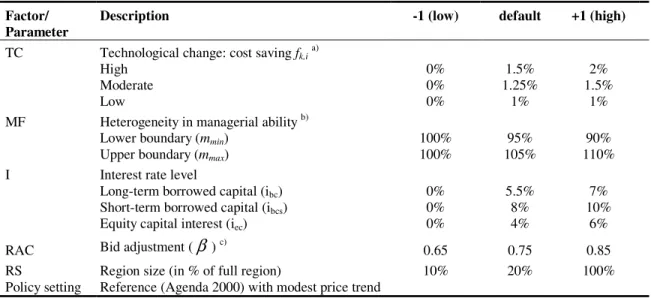
Table 1. Factors in the experimental design of the reference scenario with low (-), default, and high (+) factor setting and selection of fixed key parameters

Factor/

Parameter Description -1 (low) default +1 (high)

TC Technological change: cost saving fk,ia)

High 0% 1.5% 2%

Moderate 0% 1.25% 1.5%

Low 0% 1% 1%

MF Heterogeneity in managerial ability b)

Lower boundary (mmin) 100% 95% 90%

Upper boundary (mmax) 100% 105% 110%

I Interest rate level

Long-term borrowed capital (ibc) 0% 5.5% 7%

Short-term borrowed capital (ibcs) 0% 8% 10%

Equity capital interest (iec) 0% 4% 6%

RAC Bid adjustment (

β

RS Region size (in % of full region) 10% 20% 100%

Policy setting Reference (Agenda 2000) with modest price trend

Notes: a) Cost saving due to investment differentiated by size of investment; b) Heterogeneity of farms regarding cost structure as deviation from average (value < (>) 100% corresponds to low (high) cost producer); c) Factor determining the share of a bid which is actually paid as rent for a plot.

All selected factors are quantitative in nature. Two out of five factors represent parameter bundles (I, TC). These factors as well as factors RS, and RAC enter AgriPoliS as single values. The factor MF (managerial ability) enters AgriPoliS as limits of a rectangular probability distribution. From this distribution, values are assigned to each farm agent at the beginning of the simulation. All initialised factor levels are assumed to remain constant during the following simulation experiments. For each factor, a low and high level was defined, reflecting uncertainty about these factors in real life. The low and high values were based on expert opinion, statistical data and plausibility arguments. Obviously, the low interest rates, i.e. zero interest rates, is less realistic, if the goal is to set factor settings corresponding to what could happen in reality. But, it was chosen in order to examine how AgriPoliS behaves at the extreme of zero interest rates. These factor levels determine the relevant experimental framework for the DOE analysis. Factors not included in the DOE are assumed to remain fixed during the simulations. Table 2 presents the complete design matrix for the 25 _{full factorial design. The design} requires 32 design points or scenarios. To compare factor effects by relative importance, factor levels were set at "-" (low value) and "+" (high value) (Law and Kelton 1991).

Although AgriPoliS produces a multitude of responses, only one response variable, namely average economic land rent per hectare in the region, is chosen for analysis. Economic land rent is a central indicator for the economic performance of farms, and in particular for the efficiency of farming in the region (cf. Balmann, 1995) as it provides information about allocation of production factors in the region. To calculate the economic land rent, long-term opportunity costs of labour are valued at the comparative salary of an industrial worker. In this paper, a constant value of 22,400 € per AWU is assumed throughout all simulation periods are assumed. As AgriPoliS includes some stochastic

ele-ments, a tactical issue involves the number of replications for each simulation scenario. Earlier trials with the model indicated that results varied only within a comparatively small range between initialisations, although this cannot be regarded as a 'fix rule'. To draw statistically valid conclusions one would have to run a large number of repeated simulations. Furthermore, none of the many simulation experiments carried out in previous studies (e.g., Balmann, 1997; Balmann et al., 2002) produced results showing implausible irregularities between initialisations. Since computing time is the limiting factor, all scenarios are replicated only twice, which is a crude but necessary simplifica-tion.

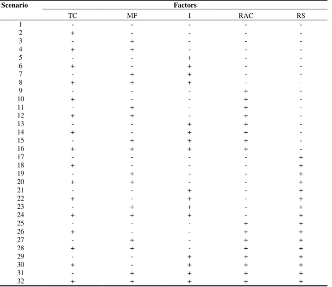
Table 2. Design matrix for the 2n _{(n=5) full factorial design}

Scenario Factors TC MF I RAC RS 1 - - - - - 2 + - - - - 3 - + - - - 4 + + - - - 5 - - + - - 6 + - + - - 7 - + + - - 8 + + + - - 9 - - - + - 10 + - - + - 11 - + - + - 12 + + - + - 13 - - + + - 14 + - + + - 15 - + + + - 16 + + + + - 17 - - - - + 18 + - - - + 19 - + - - + 20 + + - - + 21 - - + - + 22 + - + - + 23 - + + - + 24 + + + - + 25 - - - + + 26 + - - + + 27 - + - + + 28 + + - + + 29 - - + + + 30 + - + + + 31 - + + + + 32 + + + + +

Notes: Low (-), and high (+) values.

Each simulation scenario in the DOE analysis is simulated for 25 time periods. Simulation output consists of a panel data set of indicators for each individual farm in each time period and an aggregate data set for the whole region in each time period. Since the following analysis uses average economic land rent as the response variable, altogether 1600 observations could potentially be considered in the analysis (25 time periods times 32 scenarios times two replications).

A range of graphical techniques is applied to analyse simulation output of the DOE specification given in Table 2. In addition to the graphical analysis of results, a metamodel is defined to obtain some information about the statistical significance of factor effects, and in particular factor interactions. The metamodel is specified as an additive polynomial

ε

β

β

β

with the k factors as independent variables, where y is the simulation response. The intercept is 0

β

β

β

The x's denote settings of factor scenario n, and finally there is an error term

ε

4 Results

4.1 Graphical analysis

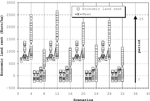
A plot of the response variable average economic land rent (mean of two replications) against all 32 scenarios and time periods shows some evidence for structure in the data (Figure 1). The figure has to be read from bottom to top for each scenario as this describes the development of economic land rent over time. The upwards pointing arrow shows the direction in which the simulation response develops over 25 simulation periods, i.e. each column contains 50 boxes (2 replications x 25 periods).

-500 0 500 1000 1500 2000 2500 3000 0 4 8 12 16 20 24 28 32 36 40 Scenarios E c o n o m i c l a n d r e n t ( E u r o / h a )

Economic land rent Mean p e r i o d 1 25

Figure 1. Scatter plot of individual and mean simulation response of two replications of 25 simulation periods against all 32 scenarios (Source: Own figure.)

In particular, three aspects can be identified: First, there is a strong and consistent pairing of the response variable: four high responses, followed by four low responses. Looking at the design matrix in Table 2, this pattern follows the level changes of factor I, which is the overall interest rate level. Higher interest rates therefore cause a decrease in economic land rent. This corresponds to what could have been expected to happen, namely that at zero interest rates economic land rent is high because of no capital costs. Second, within each block of four scenarios, one can observe that at high interest rates (e.g. scenarios 5 through 8) neither heterogeneous managerial ability nor technical change by

themselves lead to a strong increase in economic land rent. But, if both factors are at their "+" level, then the effect is large. In other words, heterogeneous managerial ability together with higher techno-logical change leads to a substantial increase in economic land rent. The same line of reasoning holds for the low interest rate level (e.g. scenarios 1 through 4). However, if interest rates are low,

heterogeneous managerial ability taken on its own also increase economic land rent. Hence, there appears to be some interaction between factors TC, MF, and I. Third, within each block of 16 scenarios (factor level change of RS), it shows that the spread of results decreases if the region size is large and interest rates low. But, at high interest rates, there is hardly any difference between a small and a large region.

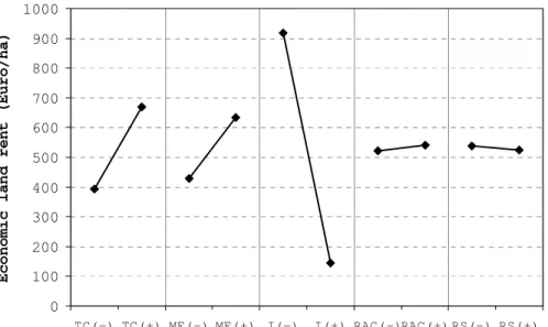
The following figures shall retrieve some more information on the relative importance of individual factors. Already in Figure 1, it could be seen that there are clear differences in results between factor level combinations. Figure 2 shows a so-called mean plot (all plots have been produced using the special DOE feature in DATAPLOT by NIST/SEMATECH 2003) which represents a simple way to identify important factors. The vertical axis shows the mean response for a given setting ("-" or "+") of a factor calculated across all scenarios, for each of k factors. The horizontal axis shows the k factors with two factor settings. For example, mean economic land rent across all scenarios with factor setting TC"-" is approximately 400 €/ha. This increases to about 680 €/ha if technological change is higher. In view of that, the difference between mean responses when moving from the "-" setting to the "+" setting of a factor is most obvious for factor I, followed by factors TC and MF.

0 100 200 300 400 500 600 700 800 900 1000

TC(-) TC(+) MF(-) MF(+) I(-) I(+) RAC(-)RAC(+) RS(-) RS(+)

Factor settings Ec o no mi c la n d re nt ( Eu ro /h a)

Figure 2. Mean plot of main effects (Source: Own figure).

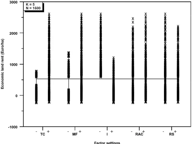
Figure 3 gives some additional information on factor importance. A factor is considered

important if it leads to a significant shift in either the location or the change in variation (spread) of the response variable as one goes from the "-" setting to the "+" setting of the factor. On the one hand, a large shift with only little overlap in the body of the data between the "-" and the "+" setting (such as for factor I) would imply that the factor is important with respect to location. On the other hand, a small shift with much overlap would imply that the factor is not important. Accordingly, Figure 3 shows a large difference between the degree of overlap between factors TC, MF, I, on the one hand, and factors RAC and RS, on the other. These latter factors do not seem important because they lead to no considerable shift in location or variation of the response variable. Using the overlap criterion, factor I is the most important factor, followed by TC and MF.

Figure 3. Main effects scatter plot (Source: Own figure).

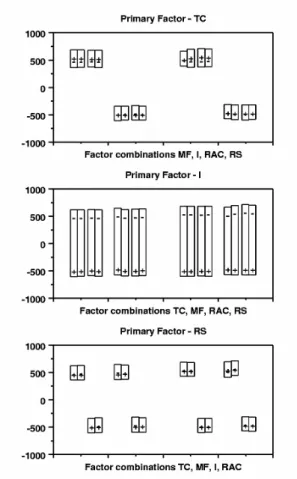
Finally, the block plot shown in Figure 4 wraps up the graphical analysis of effects. In addition to scatter and mean plots, block plots are useful to establish the robustness of main effects, and to determine factor interactions. The vertical axis shows the response variable, average economic land rent. The horizontal axis of each sub-plot shows all 2k-1 _{possible factor combinations of the (k-1)}

non-primary factors ('robustness' factors). For example, for the block plot focussing on non-primary factor I, the horizontal axis consists of all 25_{-1=16 combinations of factors MF, I, RAC, and RS. To read the figure} correctly it is important to note that a block's height determines factor importance.

Hence, factor I is most important because all bar heights in plot 3 (target factor I) are greater than bar heights in all other plots. Also, bar heights in plots 1 and 2 (target factors TC and MF) are slightly greater than bar heights in plots 4 and 5 (target factors RAC and RS), indicating that factors TC and MF are more important than factors RAC and RS. A clear ranking of factor importance is not possible, though. Plot 3 (target factor I) has the consistently largest block heights along with a consistent arrangement of within-block +'s and –'s. This indicates that factor I also was the most robust factor of all five factors considered. Factors TC and MF were not robust across the whole range of factor variations, but robust across variations of factors RAC and RS.

Figure 4. Block plot of main and interaction effects (Source: Own figure).

4.2 Metamodel analysis

To derive some statistical conclusions about factor effects, the linear regression metamodel defined in equation 1 is applied in which the average economic land rent of 25 simulation periods is regressed on factor level settings and two-factor interactions. As Figure 1 showed, the means display differences between scenarios quite well. Because each simulation scenario is replicated twice, altogether 64 data points enter the regression analysis. Results are presented in Table 3, which only lists factors significant at the 1% level.

Table 3. Factor effects based on OLS regression

Factor Estimate Standardised

estimate Standard error Significance level t-values

Constant 682.410 12.781 0.000 53.393 I -773.819 -0.884 8.073 0.000 -95.730 TC 277.290 0.317 8.073 0.000 34.304 MF 203.521 0.232 8.073 0.000 25.178 TC x I -168.267 -0.192 8.073 0.000 -20.816 TC x MF 127.144 0.145 8.073 0.000 15.729 I x RS -19.275 -0.022 8.073 0.021 -2.385 RAC 18.353 0.021 8.073 0.027 2.270 MF x RS 16.694 0.019 8.073 0.044 2.065 RS 16.265 0.019 8.073 0.049 2.012 adj. R2 _{0.995 N=64}

Notes: The dependent variable is the average economic land rent across all periods. Standard errors on estimates are the same for all independent variables except for the intercept because the model was estimated for a full-factorial design in which 50% of the observations for each factor had a high and a low value. Source: Own estimation.

Accordingly, three out of five factors are highly significant at p<0.01 (I, TC, and MF). The estimates reproduce what already could be seen in the graphical analysis when changing a factor from its "-" to its "+" setting. In other words, a factor level change of factors I, TC, and MF significantly change the development of economic land rent. The regression model appears to account for almost all the variability in the response, achieving an adjusted R2_{=0.995. The results underline the strong effect}

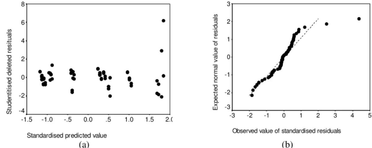
of factor I. As was expected already from the analysis of Figure 1, factors TC, MF, and I, and interactions between these factors are most important. Results also support the finding that these factors are more important than, for example, the size of the region if economic land rent is taken as the response variable. To further test the validity of the metamodel, regression residuals are analysed. Figure 5(a) shows studentitised deleted residuals plotted versus standardised predicted values of cumulative economic land rent (cf. SPSS 1999).

Approximately four out of 64 data points lie outside the interval between -2 and +2 indicating that the model could be accepted on the grounds of this plot (see SPSS 1999). The normal probability plot in Figure 5(b) shows that the distribution of residuals deviated in parts from a normal distribution underlying the metamodel. Accordingly, results of the metamodel have to be treated with care. At most, they point out a general direction. The results on the other hand do not provide strong enough evidence to reject the model as a whole, particularly, since results are supported clearly by the graphical analysis.

Standardised predicted value

2.0 1.5 1.0 .5 0.0 -.5 -1.0 -1.5 S tu de nt iti se d de le te d re si tu al s 8 6 4 2 0 -2 -4

Observed value of standardised residuals 5 4 3 2 1 0 -1 -2 -3 E xp ec te d no rm al v al ue o f r es id ua ls 3 2 1 0 -1 -2 -3 (a) (b)

Figure 5. Residual plots. (a) Scatter plot of studentitised deleted residuals versus standardised predicted values; (b) Q-Q normal probability plot (Source: Own figure).

5 Summary and conclusions

Although the selection of factors is somewhat arbitrary and based upon reasoning, the size of the impact of the significant factors shows that a deeper analysis is indeed meaningful, in particular with respect to the identification of factor interaction effects. The applied methodology and the metamodel provide a more systematic analysis of results of complex simulation models. When summarising the results, it becomes clear that interest rates, technical change and managerial ability influence average economic land rent the most. The size of the region has a much lower impact on economic land rent than expected beforehand. Other analyses in which farm incomes, rental prices, and farm size were taken as response variables confirm this. Due to limited space, these results are not reported here. In addition, factor RAC has no significant impact on results.

A problem of DOE is that no defined rules for appropriate factor level settings are given. Because of this, the importance of factors is partly based on what is defined in the experimental setup. In the extreme, if a narrow range is imposed on an important factor, but a wide range on an unimportant factor, then the latter could turn out to be more important than the former (VonkNoordegraafet al. 2002). Therefore, the fact that interest rates had such an immense influence on model outcomes could partly be explained by the fact that a wide range for the parameter setting was assumed. However, the wide range imposed on factor RS did not lead to an overestimation of the effect of region size. Nevertheless, the procedure presented here reveals some information about the importance and interactions of factors that would not have become as apparent if other designs such as varying only one factor at a time had been chosen. By applying a systematic procedure such as DOE and

metamodelling, some additional insights can be obtained about a complex simulation model such as AgriPoliS, adding to the model's validity.

References

Balmann, A. (1995). Pfadabhängigkeiten in Agrarstrukturentwicklungen – Begriff, Ursachen und Konsequenzen. Berlin: Duncker und Humblot.

Balmann, A. (1997). Farm-based Modelling of Regional Structural Change: A Cellular Automata Approach,

European Review of Agricultural Economics 24(1): 85-108.

Balmann, A., Happe, K., Kellermann, K., Kleingarn, A. (2002). Adjustment Costs of Agri-Environmental Policy Switchings: An Agent-Based Analysis of the German Region Hohenlohe. In Janssen, M.A. (ed),

Complexity and ecosystem management – the theory and practice of multi-agent systems. Cheltenham,

Northhampton: Edward Elgar, 127-157.

Box, G.E.P, Hunter, W. G., Hunter, J. S. (1978). Statistics for Experimenters: An Introduction to Design, Data

Analysis and Model Building. New York, Chichester: John Wiley.

Happe, K., Balmann, A., Kellermann, K. (2004). The Agricultural Policy Simulator (AgriPoliS) – An Agent-Based Model To Study Structural Change in Agriculture (version 1.0). IAMO Discussion Paper 71. [http://www.iamo.de/dok/dp71.pdf]

Happe, K. (2004). Agricultural policies and farm structures – agent-based modelling and application to

EU-policy reform. Studies on the Agricultural and Food Sector in Central and Eastern Europe, vol. 30, IAMO.

[http://www.iamo.de/dok/sr_vol30.pdf]

Law, A.M., Kelton, W.D. (1991). Simulation modelling and analysis. 2nd edition, McGraw-Hill, New York, St. Louis.

Kleijnen, J.P.C. (1999): Validation of models: statistical techniques and data availability. In Farrington, P.A., Nembhard, H.B., Sturrock, D.T., Evans, G.W. (eds) Proceedings of the 1999 Winter Simulation

Conference. [http://www.informs-cs.org/wsc99papers/prog99.html]

Kleijnen, J.P.C., Sanchez, S.M., Lucas, T.W., Cioppa, T.M. (2003). A user's guide to the brave new world of designing simulation experiments, CentER Discussion paper No. 2003-01, Tilburg University.

Kleijnen, J.P.C., Groenendaal, W. van (1992). Simulation – a statistical perspective. New York, Chichester: John Wiley.

Lempert, R.J., Schlesinger, M.E., Bankes, S. (1996). When We Don't Know the Costs ort he Benefits: Adaptive Strategies for Abating Climate Change. Climatic Change 33: 235-274.

Manson, S.M. (2002). Validation and verification of multi-agent systems. In Janssen, M.A. (ed), Complexity and

ecosystem management – the theory and practice of multi-agent systems. Cheltenham, Northhampton:

Edward Elgar, 63-74.

NIST/SEMATECH Methods (2003). e-Handbook of Statistical, Retrieved from internet July 2003, http://www.itl.nist.gov/div898/handbook/.

Sanchez, S.M., Lucas, T.W. (2002). Exploring the world of agent-based simulations: simple models, complex analyses. In Yücesan, E., Chen, C.-H., Snowdon, J.L., Charnes, J.M (eds), Proceedings of the 2002 Winter

Simulation Conference. [http://www.informs-cs.org/wsc02papers/prog02.htm].

Sargent, R.G. (2004). Validation and verification of simulation models. In Ingalls, R.G., Rossetti, M.D., Smith, J.S., Peters, B.A. (eds), Proceedings of the 2004 Winter Simulation Conference. [http://www.informs-sim.org/wsc04papers/004.pdf]

SPSS Base 10.0 Applications Guide (1999).

Vonk Noordegraaf, A., Nielen, M., Kleijnen, J.P.C. (2002). Sensitivity analysis by experimental design and metamodeling: case study on simulation in national animal disease control. European Journal of