Aggregate fluctuations and the network structure of intersectoral trade

Aggregate Fluctuations and the Network

Structure of Intersectoral Trade

Vasco M. Carvalho

October 28, 2010

Abstract

This paper analyzes the ‡ow of intermediate inputs across sectors by adopting a net-work perspective on sectoral interactions. I apply these tools to show how ‡uctuations in aggregate economic activity can be obtained from independent shocks to individual sectors. First, I characterize the network structure of input trade in the U.S.. On the demand side, a typical sector relies on a small number of key inputs and sectors are homogeneous in this respect. However, in their role as input-suppliers sectors do di¤er: many specialized input suppliers coexist alongside general purpose sectors functioning as hubs to the economy. I then develop a model of intersectoral linkages that can re-produce these connectivity features. In a standard multisector setup, I use this model to provide analytical expressions linking aggregate volatility to the network structure of input trade. I show that the presence of sectoral hubs - by coupling production decisions across sectors - leads to ‡uctuations in aggregates.

Keywords: Aggregation; Business Cycles; Comovement; Input-Output; Multisector Growth Models; Networks; Technological Diversi…cation

CREI and U. Pompeu Fabra. For comments and contact, please mail at [email protected]. This paper draws from material in my 2008 University of Chicago dissertation. I thank my advisor, Lars Hansen, and my committee members, Robert Lucas and Timothy Conley. For comments and encouragement I thank Daron Acemoglu, Fernando Alvarez, Luis Amaral, Susantu Basu, Paco Buera, Yongsung Chang, Antonio Ciccone, John Fernald, Xavier Gabaix, Jordi Gali, Yannis Ioannides, Matthew Jackson, Boyan Jovanovic, Marcin Peski, Pierre-Daniel Sarte, Thomas Sargent, Hugo Sonnenschein, Jaume Ventura, Randall Verbrugge and seminar participants at the Bank of Portugal, Boston Fed, Carnegie-Mellon, CREI, UC Davis, EEA, Econometric Society, EIEF, U Montreal, NBER Summer Institute, NY Fed, NYU/Stern School, Rochester, SED. I acknowledge …nancial support from the Government of Catalonia (grant 2009SGR1157), the Spanish Ministry of Education and Science (grants Juan de la Cierva, JCI2009-04127, ECO2008-01665 and CSD2006-00016) and the Barcelona GSE Research Network.

1

Introduction

Comovement across sectors is a hallmark of cyclical ‡uctuations. A long-standing line of research in the business cycle literature asks whether trade in intermediate inputs can link otherwise independent technologies and generate such behavior. The intuition behind this hypothesis is clear: factor demand linkages can provide a source for comovement, as a shock to the production technology of a general purpose sector - say, petroleum re…neries - is likely to propagate to the rest of the economy. In this way, cyclical ‡uctuations in aggregates are obtained as synchronized responses to changes in the productivity of narrowly de…ned but broadly used technologies.

Though intuitive, this hypothesis is faced with a strong challenge: by a standard diversi-…cation argument, as we disaggregate the economy into many sectors, independent sectoral disturbances will tend to average out, leaving aggregates unchanged and yielding a weak propagation mechanism; see the discussion in Lucas (1981) and the irrelevance theorems of Dupor (1999)1_.

In this paper, I take on this challenge by adopting a network perspective on sectoral interactions. From this vantage point, I provide answers to the following questions. First, given the availability of detailed input use data, can we identify the main features of the network structure of linkages across sectors? Second, can we specify models of sectoral input linkages that are able to mimic this connectivity structure and are still amenable to use in standard multi-sector models? If so, can we use these models to derived analytical results linking the variability of aggregates to the network structure of input ‡ows? Finally, under what assumptions on the network structure can we render ine¤ective the shock diversi…cation argument of the previous paragraph?

The argument linking the answers to these questions is the following: when determining whether a sectoral shock propagates or not, the number of sectoral connections originating from the source of the shock is the crucial variable to consider. Furthermore, if the number of 1_{For the most part, the answer to this challenge has been in the empirical vein. Long and Plosser (1983,} 1987), Norrbin and Schlagenhauf (1990) and Horvath and Verbrugge (1996) document comovement of sectoral output growth series through vector autoregressions. They all add that the explanatory power of a common, aggregate shock is limited on its own and diminished once sector speci…c shocks are entertained. Shea (2002) and Conley and Dupor (2003) go further and devise ways of testing - and rejecting- the hypothesis that sectoral comovement is being driven by a common shock. Concurrently, the strategy of using actual input-output data in large scale multisector models generates aggregates that are quantitatively similar to data and to one-sector real business cycle models; see Horvath (2000).

connections varies widely across sectors, some shocks will propagate throughout the economy and persist through time while others will be short-lived and only propagate locally. As a consequence, economies where every sector relies heavily on only a few sectoral hubs - general purpose input suppliers - will show considerable conductance to shocks in those technologies. Conversely, as the structure of the economy is more diversi…ed, di¤erent sectors will rely on di¤erent technologies and exhibit only loosely coupled dynamics. The answer to the law of large numbers arguments in Lucas and Dupor thus lies in understanding and modelling this tension between specialization and reliance on general purpose technologies.

A simple example - a particular case of the setup in Shea (2002)- helps build intuition for this tension2_{. Consider an economy where a representative household derives log utility} overM sectoral goods and linear disutility from time spent working. Each of the M sectors produce a di¤erent good that can either be allocated to …nal consumption or as an interme-diate input to the production of other goods. In particular, let the production side of this economy be given byM;Cobb-Douglas, constant returns to scale production functions, each combining labor and a distinct set of intermediate inputs. Finally, assume that each sector is subject to a productivity shock of variance 2 _{but insist that these shocks areindependent}

realizations across sectors.

Whether these shocks will then propagate through input linkages and lead to movements in aggregates depends on the network structure of these linkages. To see this, consider the two following abstract, and rather extreme, cases. Fix anM and contrast an economy where only one sector is a material input supplier to all other sectors with an economy where every sector supplies to all other sectors in the economy. These two polar cases for the pattern of input-use relationships in an economy map exactly into very standard network representations, where the vertex set is given by the set of sectors in the economy and a directed arc from vertex (sector) ito vertex j represents a intermediate input supply link.

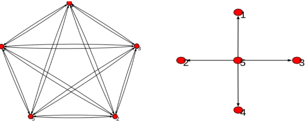
1 2 3 4 5 P ajek 5 1 2 3 4 Pajek

Figure 1: Complete (l.h.s.) and Star (r.h.s.) input-supply structures for a 5 sector economy.

Thus an economy where each sector is an input supplier to every other sector in the economy can be represented by acomplete network, where for any two pair of vertices there is a directed arc from one to the other. Likewise, an economy where there is only one material input supplier maps directly into a star network, where one vertex acts as a hub with directed arcs from this vertex to all other vertices. An intermediate case is given by a

N star network, where N out of M, sectors in the economy act as material input suppliers to every sector and the remaining ones are solely devoted to …nal goods production. Figure 1 depicts intersectoral input relations under these two extreme cases complete and star -for a …ve sector economy.

In order to focus on the impact of heterogeneity along the extensive margin of intersectoral trade, assume further that, each sector, regardless of what its particular input list is, uses its inputs in equal proportions. Then, de…ning aggregate volatility, 2_Y; as the variance of average log output, I show that 2

Y _

2

M for the case of complete networks while

2

Y _

2 N

for the case of N star networks.

Thus, aggregate volatility with complete intersectoral networks echoes Dupor’s and Lu-cas’ law of large numbers argument: aggregate volatility scales with 1=M. To understand how e¤ective the shock diversi…cation argument is notice the following: holding sectoral variance …xed as I move from a …ve sector economy to a …ve hundred sector economy, ag-gregate volatility will be a hundred times smaller. Conversely, to recover an agag-gregate 2

Y of

the order of two percent in a …ve hundred sector economy, would require stipulating sectoral volatilities, 2_{;to be …ve hundred times larger, an unreasonable magnitude at any time scale.}

However, if there are only N sectors acting as intermediate input suppliers, the diversi-…cation of shocks argument underlying law of large number arguments only applies to those

sectors. Thus, in an economy where the e¤ective number of input suppliers is small, the law of large numbers will be postponed relative to that of Dupor (1999): aggregate volatility now scales with 1=N. This is Horvath’s (1998) argument: limited sectoral interaction - of a very particular form - will give rise to greater aggregate volatility from sector speci…c shocks. The di¢ culty with this result is that the modeler is now left to specify, for each M;what is the number of input suppliers in an economy; N. From input-output data, Horvath (1998) argues that N - the number sectors with full rows in input-output matrices - grows slowly with M: Horvath argues for an N of order pM. This would now yield a ten fold decrease in aggregate variability as we move from …ve to …ve hundred sectors.

In this way, two very particular assumptions on the network structure of intersectoral trade generate predictions on the variability of aggregates that di¤er by an order of magni-tude. This means that …nding a better way to model networks of input trade can not only help solve this controversy but also has the potential of o¤ering a theory where reasonable magnitudes of sectoral volatility yield non-trivial aggregate volatility. Mechanically, we need only a theory of intersectoral connectivity that yields aggregate volatility decaying withM ;

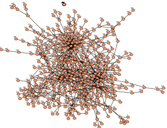
where is close to zero. This paper does just this by going beyond these two extreme cases and building a model of sectoral interactions on a network. Figure 2 depicts the starting point of the analysis. It shows a considerably more intricate network of intersectoral input ‡ows: that of the U.S. economy in 1997.

Each dot - or vertex - corresponds to a sector de…ned at the NAICS 4-6 digit level of disaggregation in the BEA detailed commodity-by-commodity tables, for a total of 474 sectors. Each link in the …gure represents an input transaction between sectori to sector j, provided sector i supplies more than 5% of sectorj total intermediate input purchases3_.

3_{I exclude loops from the network for presentation purposes. Loops correspond tointrasectoral trade and} are a well documented feature of detailed input use-matrices (see for example Jones, 2010b).

1 2 3 4 5 6 7 8 9 10 11 12 13 14 15 16 17 18 19 20 21 22 23 24 25 26 27 28 29 30 31 32 33 34 35 36 37 38 39 40 41 42 43 44 45 46 47 48 49 50 51 52 53 54 55 56 57 58 59 60 61 62 63 64 65 66 67 68 69 70 71 72 73 74 75 76 77 78 79 80 81 82 83 84 85 86 87 88 89 90 91 92 93 94 95 96 97 98 99 100 101 102 103 104 105 106 107 108 109 110 111 112 113 114 115 116 117 118 119 120 121 122 123 124 125 126 127 128 129 130 131 132 133 134 135 136 137 138 139 140 141 142 143 144 145 146 147 148 149 150 151 152 153 154 155 156 157 158 159 160 161 162 163 164 165 166 167 168 169 170 171 172 173 174 175 176 177 178 179 180 181 182 183 184 185 186 187 188 189 ₁₉₀ 191 192 193 194 195 196 197 198 199 200 201 202 203 204 205 206 207 208 209 210 211 212 213 214 215 216 217 218 219 220 221 222 223 224 225226 227 228 229 230 231 232 233 234 235 236 237 238 239 240 241 242 243 244 245 246 247 248 249 250 251 252 253 254 255 256 257 258 259 260 261 262 263 264 265 266 267 268 269 270 271 272 273 274 275 276 277 278 279 280 281 282 283 284 285 286 287 288 289 290 291 292 293 294 295 296 297 298 299 300 301 302 303 304 305 306 307 308 309 310 311 312 313 314 315 316 317 318 319 320 321 322 323 324 325 326 327328 329 330 331 332 333 334 335 336 337 338 339 340 341 342 343 344 345 346 347 348 349 350 351 352 353 354 355 356 357 358 359 360 361 362 363 364 365 366 367 368 369 370 371 372 373 374 375 376 377 378 379 380 381 382 383 384 385 386 387 388 389 390 391 392 393 394 395 396 397 398 399 400 401 402 403 404 405 406 407 408 409 410 411 412 413 414 415 416 417 418 419 420 421 422 423 424 425 426 427 428 429 430 431 432 433 434 435 436 437 438 439 440 441 442 443 444

Figure 2: Intermediate input ‡ows between sectors in the U.S. economy in 1997. Each vertex corresponds to a sector in the 1997 benchmark detailed commodity-by-commodity direct requirements matrix (Source: BEA). For every input transaction above 5% of the

total input purchases of the destination sector, a link between two vertices is drawn.

From this vantage point, Section 2 in the paper o¤ers a two-pronged characterization of the structure of input ‡ow data by taking into consideration the direction in each of these links. Thus, by considering links from the perspective of the destination vertex, I can analyze sectors in their role as input-demanders. I …nd that sectors are homogeneous along this dimension: the typical sectoral production technology relies on a relatively small number of key inputs and sectors do not di¤er much in this respect. This is the upshot of specialization occurring at the level of narrowly de…ned production technologies.

However, looking at the source vertices of these links, another feature emerges: extensive heterogeneity across sectors in their role as input suppliers. In the data, highly specialized input suppliers - say, for example, optical lens manufacturing - coexist alongside general purpose inputs, such as iron and steel mills or petroleum re…neries. Speci…cally, I characterize the empirical out-degree distribution of input-supply links - giving the number of sectors to which any given sector supplies inputs to - as a power law distribution. What makes this power law parameterization attractive is the following argument: the upshot of fat-tails, characteristic of power law degree distributions, is that a small, but non-vanishing, number

of sectors will emerge as large input suppliers - or hubs - to the economy.

In Section 3, I construct a network model of intersectoral linkages that is able to incorpo-rate these two …rst order-features of the data: sparse and homogeneous input demand and strongly heterogenous input supply technologies. Returning to the static multisector setup described above, I then show that whenever the network of input linkages incorporate these two features convergence of aggregate volatility to zero can be slowed down dramatically. In particular, I show that in this setup 2

Y _ 2

1

M

2 4

1 _where

2 (2;3) is the tail parameter on the power law distribution of input-supply linkages. Given the empirical characteriza-tion of Seccharacteriza-tion 2, = 2:1 seems to be a good description of actual input-use data. Thus,

2

Y _ 2

1

M

0:18

. This means that going from a …ve to a …ve-hundred sector economy - while keeping sector-level volatility constant - now implies that aggregate volatility is reduced only

two-fold. Alternatively, we need only that the typical sectoral volatility of narrowly de…ned sectors be double than that of more aggregated sectors for aggregate volatility to remain constant across these two economies.

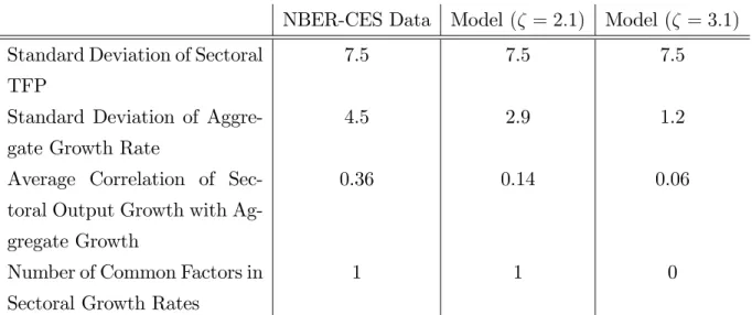
The remainder of the paper (Section 4) is devoted to verifying that these claims still hold in standard, dynamic, multisector setups. In particular, I show that the decay character-ization above extends to the auto-covariance function of aggregate output growth. I then present some quantitative explorations in this class of models and claim that the mecha-nisms described in this paper are quantitatively relevant: a large scale multisector model with independent shocks can generate aggregate volatility that is about two-thirds of that observed in data.

The paper is closest to the contribution of Gabaix (2010) and to the independent, but sub-sequent, work by Acemoglu, Ozdaglar and Tahbaz-Saleh (2010). Regarding Gabaix (2010), this paper is closely related to his characterization of aggregate volatility decay as a function of heterogeneity in the underlying production units. In contrast to Gabaix however, this is not the result of some …rms accounting for a non-trivial share of aggregate output and thus, for a non-trivial share of aggregate volatility. Rather the argument here is based on the shock conductance implied by the interlocking of technologies in a networked economy. In other words, the emphasis here is on propagation rather than aggregation. These two approaches should therefore be seen as a complementary. Acemoglu et al (2010), consider a networked, static, multisector economy which is very similar to the one discussed earlier in this introduction and expanded further upon in Section 3. They use a di¤erent approach (deterministic graphs, rather than the random graphs setup used here) which allows them to con…rm the volatility decay behavior discussed above - stated in Proposition 2 of this

paper- and then analyze higher-order network e¤ects and the possibility of tail events in the aggregate. They do not study whether this is still the case in dynamic settings which allow for richer interactions due to the presence of capital accumulation - as is done here- nor do they look at the quantitative implications of these settings.

The underlying multi-sector setup that I use is very close to that appearing in Horvath (1998), Dupor (1999), Shea (2002) and Foerster, Sarte and Watson (2008), all closely related to the original multisector real business cycle model of Long and Plosser (1983) and the myr-iad of extensions and applications developed in the literature since. Much of this literature has used actual input-output data in the calibration of more complicated large-scale multi-sector equilibrium models with some quantitative success; see Horvath (2000), Kim and Kim (2006) or Bouakez, Cardia and Ruge-Murcia (2009) for examples of this. This papers asks what in the nature of input-output data is enabling such results, unexpected in a context of independent sectoral shocks.

The paper is also close to the spirit of the contributions in Bak et al.(1993) and Scheinkman and Woodford (1994) by stressing the importance of the structure of input-supply chains in the transmission of shocks across sectors and, as a consequence, to aggregates. In comparison with these papers, by placing sectors on a network of input ‡ows - rather than on a lattice - I allow for more general, and arguably more realistic, patterns of connections between sec-tors4_{. The idea of characterizing input-use relationships through graph-theoretical tools is} not new, albeit it has merited only limited attention5_{. In the context of traditional} input-output analysis Solow (1952) is, to the best of my knowledge, the …rst reference recognizing that an input-output matrix can be mapped into a network. These tools have resurfaced only sporadically in the analysis of static and dynamic input-output systems; see Rosenblatt (1957), Simon and Ando (1961) or Szydl (1985).

In terms of tools, this paper borrows heavily from recent work on networks and in par-ticular, random graphs. Newman (2003) and Li et al (2006) o¤er good reviews mapping out recent theoretical advances and link them to a growing number of applications. Durrett (2006) and Chung and Lu (2006) provide textbook treatments. In particular, a model of 4_{Other related setups have been explored in order to generate aggregate ‡uctuations from micro shocks:} Cooper and Haltiwanger (1990). Jovanovic (1987) and Durlauf (1993) instead focus on the role of production complementarities across sectors, as does the more recent contribution of Nirei (2005), where this is coupled with indivisibilities in investment. In turn, Murphy et al. (1989) focus on aggregate demand spillovers.

5_{This stands in sharp contrast to the recent but burgeoning use of network tools in microeconomics; see} Jackson (2005) for a comprehensive review or Vega-Redondo (2007), Jackson (2008) or Goyal (2009) for monographs on the topic.

random graphs with given expected degree sequences, set out in Chung and Lu (2006), forms the basis for my data-generating process for intersectoral linkages.

2

Network Properties of Input Flow Data

This section conducts an empirical analysis of some network properties of input ‡ow data. Throughout, I use detailed Benchmark Input-Output data compiled by the Bureau of Eco-nomic Analysis, spanning the period 1972-2002. The detailed input-output data yield a …ne disaggregation of inter-sectoral trade, most sectors corresponding to (roughly) a four digit S.I.C. de…nition. The data is made available on a …ve year interval.6

In particular, I use the commodity-by-commodity direct requirements tables7 _{where the} typical (i; j) entry gives the input-share (evaluated at current producers’ prices) of (row) commodityias an intermediate input in the production of (column) commodityj. Abusing notation slightly, I use the names commodities and sectors interchangeably throughout the paper (i.e. I assume that commodityi is produced exclusively by sectori).

I now map this intersectoral input trade data into standard graph theoretical notation. First, let the set of M sectors in an economy give the set of …xed labels for the vertex set

V =: _fv1; :::; vMg. Let E be a subset of the collection of all ordered pairs of vertices fvi; vjg;

with vi; vj 2V. De…ne E by:

f fvi; vjg 2V2 :fvi; vjg 2E if Sector i supplies Sector jg

That is, the edge set E; is given by an adjacency relation, vi ! vj between elements of

the set of all sectors where I allow re‡exivity (a sector can be an input supplier of itself). With the collectionV of sectors and input supply relationsE;I de…ne sectoral trade linkages as a directed graphG:

De…nition 1 G= (V; E). G is a directed sectoral linkages graph with vertex set V and edge set E where each element of E is a directed arc from element i to j .

6_{Up until 1992, it is based on an evolving a S.I.C. classi…cation whereas the NAICS system was adopted} from 1997 on. See Lawson et al. (2002) for a comparison of the two classi…cation systems and in-depth dis-cussion of the data. While individual sectors are not immediately comparable between S.I.C. and N.A.I.C.S., the network structure of these matrices will be shown to be remarkably stable across classi…cation systems. 7_{These are not available for all benchmark years but are possible to construct using the available Use and} Make tables following the indications in Shea (1991) or the BEA’s own Input-Output manual (Horowitz and Planting (2006)).

A useful representation of a graph is its adjacency matrix, indicating which of the vertices are linked (adjacent). This will be a key object in the sections below and is de…ned by: De…nition 2 For a directed sectoral linkages graph G(V; E) de…ne the adjacency matrix

A(G) to be an M M matrix. If G is a directed graph de…ne the aij element of A(G) to

be 1 if there is a directed edge from sector i to sector j (i.e. if sector i is a material input supplier of j) and zero otherwise.

I now characterize the extent of heterogeneity along the extensive margins of input de-mand and input supply. In particular, I consider the number of di¤erent inputs a sector

demands in order to produce- as measured by the columns sums of the adjacency matrix

A(G) - and the number of di¤erent sectors a sectorsupplies inputs to - as measured by the row sums of A(G): These count measures can be mapped directly in two graphical objects, namely the indegree and outdegree sequences of an intersectoral graphG:

De…nition 3 The in-degree din_i of a vertex vi 2 V is given by the cardinality of the set

fvj :vj !vig: The in-degree sequence of a graph G(V; E) is given by fdin1 ; :::; d in

Mg:

Figure 3 below, displays the empirical density of sectoral indegrees for every detailed matrix available since 1972. I de…ne the indegree of a sectorias the number of distinct input-demand transactions that exceed 1% of the total input purchases of that sector. By only counting as links input transactions above 1% of a sector’s total purchases, I am discarding very small transactions between sectors and focusing on the main components of the bill of goods necessary to the production of any given sector. Indeed, following this threshold rule, I account for about 80% of the total value of intermediate input trade in the US economy in 2002. A similar number obtains for all the other years considered8.

The demand side picture that emerges from Figure 3 is the following: the average sector in the US economy procures a non-trivial amount of inputs from only a small number of sectors (_' 15) and sectors do not di¤er much along this demand margin. In other words, the average indegree is small relative to the total number of sectors and most sectors have an indegree that is close to the average indegree.

8_{Though arbitrary, this counting convention seems necessary as there is no way of distinguishing between,} say, an input transaction from sector i to j in the order 10 million dollars and an input transaction from sector k to j two orders of magnitude above. Both get counted as one demand link of sector j. In the appendix, I show that the characterization presented here holds for alternative thresholds.

0 5 10 15 20 25 30 0 0. 02 0. 04 0. 06 0. 08 0. 1 0. 12 S ec t oral I ndegree E m pi ric a l D e n s it y 0 5 10 15 20 25 30 35 0 0. 02 0. 04 0. 06 0. 08 0. 1 0. 12 S ec t oral I ndegree E m pi ric a l D e n s it y 2002 1972 1977 1982 1987 1992 1997

Figure 3: Empirical density of sectoral indegrees. Only input demand transactions above 1% of the demanding sector’s total input purchases are counted. On the l.h.s. is the indegree

density for the 2002 detailed direct requirements IO matrix; on the r.h.s. are the empirical densities for direct requirements matrices from 1972 through 1997. Source: B.E.A..

This can be seen as a way to encode a …rst-order characteristic of detailed input-output data already alluded to by Horvath (1998) and Jones (2010a and 2010b): these are sparse matrices re‡ecting specialization occurring at the level of narrowly de…ned production tech-nologies. Henceforth I’ll dub this feature as homogeneity along the extensive margin of sectoral demand. This is to be contrasted with the extreme heterogeneity found along the supply side to which I now turn.

De…nition 4 The out-degree dout

i of a vertex vi 2 V is given by the cardinality of the set fvj :vi !vjg: The out-degree sequence of a graph G(V; E) is given by fdout1 ; :::; doutM g.

Figure 4 documents the heterogeneity in sectoral supply linkages by plotting the empirical out-degree distribution in the input-use data where again I use the 1% threshold to de…ne a link. It gives a log-log rank-size plot, i.e. a log-log plot empirical counter-cumulative distribution of the outdegrees, or the probability, P(k); that a randomly selected sector supplies inputs to k or more sectors9_.

9_{The construction of these plots is standard: …rst, rank all sectors according to the total number of} sectors they supply inputs to. Now plot the log of the out-degree of each sector (in the x-axis) against its log rank (in the y-axis). To interpret the plot it is useful to notice the following: if I rank sectors then, by

100 101 102 103 10-3 10-2 10-1 100 Sectoral O utdegree E m p ir ic al C C D F 2002 10-3 10-2 10-1 100 10-3 10-2 10-1 100

Percent age of Sectors Supplied

E m p ir ic al C C D F 1997 1992 1987 1982 1977 1972

Figure 4: Counter-cumulative outdegree distribution from direct requirements detailed tables. Only input demand transactions above 1% of the demanding sector’s total input purchases are counted. On l.h.s is the 2002 data. The r.h.s. displays 1972 through 1997 data where I normalize the sectoral outdegree dout

i by the total number of sectors in each

year. Source: B.E.A.

Given that every matrix, from 1972 through 1997, di¤ers slightly in its dimensions (i.e. in the number of sectors considered), for every year through 1997, I normalize sectoral outdegrees by the total number of sectors in the input-use matrix. This enables me to compare features of the distributions across di¤erent input-use matrices by standardizing the x-axis in the r.h.s of Figure 4.

The apparent linearity in the tail of the (countercumulative) outdegree distribution in log scales is usually associated with a power law distribution10. To see this formally, let

P(k) = PM_k0=kpk0 be the countercumulative distribution of outdegrees, i.e. the probability

that a sector selected at random from the population supplies to k or more sectors. The number of sectors supplied (i.e. the outdegree), k, follows a power law distribution if, the p.d.f. pk (giving the frequency of sectors that supply to exactly k sectors in the economy) is

de…nition, there are i sectors that supply inputs to a number of sectors that is greater or equal than that of the ith _{largest sector. Thus dividing the sector’s rank i by the total number of sectors (M) gives the}

fraction of sectors larger thani.

10_{Which is also a typical feature of the …rm size distribution (see, for example, Axtell (2001), Luttmer} (2007) or Gabaix (2010)).

given by:

pk=ck for >1, and k integer, k 1

where c is a positive constant and is the tail index: Well-known properties of this dis-tribution are that for 2 < 3; k has diverging second (and above) moments11 _{while for}

1< <2; kwill have diverging mean as well. An estimate on the value of the tail parameter, , can in principle be obtained by running a simple least squares regression of the empirical log-CCDF on the log-outdegree sequence (or its normalized counterpart). However, Clauset, Shalizi and Newman (2009) show that least squares methods can produce substantially in-accurate estimates of parameters for a power-law distribution. Hence, I follow Clauset et al (2009) in implementing Hill-type MLE estimates ofbfor the tail of the distribution (i.e. using all observations on or above some endogenously determined minimum degree) obtained for every year. I also report the corresponding standard errors and the number of observations in the tail12_. 1972 1977 1982 1987 1992 1997 2002 b 2.22 2.31 2.30 2.03 2.01 2.17 2.05 s:e:(b) 0.22 0.21 0.22 0.16 0.14 0.17 0.13 N_tail 72 81 68 132 121 93 112 M 483 523 527 509 478 474 417

Table 1: MLE estimates b, their standard errors (s:e:(b)); the number of observations used to estimate the tail parameter (N_tail) and the total number of sectors (M) for each

year from 1972-2002

The straight lines in Figure 5 show the MLE …t implied byb= 2:1(the average estimate across years is 2.14). From the discussion above, this value of the tail parameter implies a strong fat tailed behavior where the variance is diverging with the number of sectors. This can be taken as a parametric characterization of another feature of input-use matrices already 11_{Though in any …nite sample a …nite variance can be computed, what this means is that the variance} diverges to+₁as the total number of sectors grows larger. (see Newman, 2003 and 2005, Li et. al., 2006 and Gabaix 2009, for useful reviews and references therein)

12_{Simple OLS estimates of or their modi…ed version as proposed in Gabaix and Ibragimov (2009)} -with an exogenously determined number of sectors on the tail (set at 20% of the number of sectors) lead to very similar point estimates. The appendix shows that when di¤erent cuto¤ rules are used to de…ne a link, similar numbers obtain. See for, example, Brock (1999), Mitzenmacher (2003) or Durlauf (2005) for further discussions on the di¢ culty of identifying power laws in data.

remarked in Horvath (1998) and Jones (2010a and 2010b): as we disaggregate the economy into …ner de…nition of sectoral technologies, large input-supplying sectors do not vanish. In other words, at the most disaggregated level of sectoral input trade, the distribution of input-supply links is fat tailed.

3

Modelling Networked Sectoral Linkages

When modelling production in a multi-sector context, explicitly accounting for the ‡ows of inputs across sectors entails specifying both a list of intermediate inputs needed for the production of any given sector and the intensity of use of each particular intermediate input in that list. In the particular setting where gross output production functions are Cobb-Douglas, this means specifying the cost shares of intermediate inputs and setting to zero these parameters when a particular input is not required for the production of a given good. According to the analysis of the previous section, one can characterize the zero patterns of these lists as restrictions on the network structure of linkages. This section …rst shows how to incorporate the two …rst order network features isolated above in the simplest multisector setup possible. I then show, analytically, how aggregate volatility depends on the network structure of intersectoral linkages.

3.1

A Static Multisector Economy

Consider the following static multisector economy, a particular case of the setup presented in Shea (2002). There is a representative household whose utility is a¤ected by the levels of consumption of M goods, _fCjgMj=1; and total hours of work ; L;to be shared among the M

production activities. Assume log preferences overM di¤erent goods, with weights given by f jgMj=1, and linear disutility of labor.

U(_fCj; LjgMj=1) = M X j=1 jlog(Cj) L; (1) with P j j = 1 and j >0;8j; (2) and P j Lj L (3)

Each of the M productive units, or sectors, produce a di¤erent good that can either be allocated to …nal consumption (by the household) or as intermediate goods to be used in

the production of other goods. This is just a static version of the production technologies introduced in Long Plosser (1983). In particular, assume production functions are of the Cobb-Douglas, constant returns to scale variety:

Yj = ZjL j j Y i2Sj M ij ij (4) 1 = _j +X i2Sj ij; j >0; j = 1; :::; M (5) Zj = exp("j); "j sN(0; 2j) (6)

where Mij is the amount of good i used as an intermediate input in the production of

sector j. Zj is a Hicks-neutral, log-normal, productivity shock to good j technology, to

be drawn independently across sectors. The ‘supply-to’set Sj completes the description of

technology in this simple economy. It gives, for every sector j; the list of goods that are necessary as inputs in the production of good i. Finally, market clearing implies that:

Yj =Cj +

X i:j2Si

Mji, j = 1; :::; M (7)

It is a standard exercise to solve for the competitive equilibrium of this economy; see Shea (2002). Substituting the equilibrium input choices into the production function, simplifying and taking logarithms yields, in vector notation:

y= +(I ) 10" (8) where is an M-dimensional vector of constants dependent on model parameters only13_. The pair of vectors M-dimensional vectors (y;") give, respectively, the log of equilibrium output and the log of the productivity shock for every sector in the economy. I is the

M M identity matrix and is an M M input-use matrix with typical element _ij 0. The jth _{column sum of gives the cost share of intermediate inputs for sector j:}

j = M X

i=1

ij

13_{The setup in Shea (2002) also considers preference shocks by making the preference weights on each good} stochastic. Shea then shows that the competitive equilibrium solution will be given by (8) plus an additional random vector in the right hand side of expression re‡ecting demand shocks propagating through the input output matrix. In the simpli…ed setup of the current paper this shocks are not present and therefore this a zero vector.

where _j <1for all j, such that the M M matrix (I ) 1 _{is well de…ned}14_{. Thus, in} this simple setup, independent technological shocks at the sectoral level propagate through the input-use matrix downstream15, a¤ecting the costs of input-using sectors and potentially in‡uencing aggregate activity. Henceforth, the analysis focuses on the interplay between the network structure of intermediate input use - the structure of the input matrix, - and the propagation of sectoral shocks, as given by the equilibrium expression (8).

The following Lemma is key for the rest of the analysis in that it yields a simple factoriza-tion of the input-use matrix into the product of two square matrices: a binary adjacency matrix A(G), giving the structure of intersectoral linkages in the economy - de…ning who trades with whom - and a diagonal matrixD setting the scale of input transactions between two sectors by de…ning the level of the cost shares for the non-zero elements of (G). Lemma 1 Assume that, for each sector j = 1; :::; M; _ij = _kj; for all inputs i and k

necessary to the production of output in sector j; that is for all pairs ij; kj 6= 0. Then, the

input-use matrix is given by:

(G) =A(G)D

where A(G) is a binary adjacency matrix representation of the intersectoral network, and

D is a diagonal matrix with a typical element Dkk = _dink k

, where _k < 1 and din

k >0 is the

indegree of sectori. Further, for any M and any A; the columns sums of (G) are given by

j <1; for j = 1; ::; M and (I (G)) 1 is well de…ned:

The proof of the Lemma follows immediately from the assumption that _ij = _kj for all

ij; kj 6= 0:This assumption will be used throughout the paper as it simpli…es considerably

the description of a sectoral technology by imposing homogeneity along the intensive margin of intersectoral trade - necessary inputs for any given sector have a symmetric role- while allowing for substantial heterogeneity along the extensive margin - sectors can di¤er in the number of sectors they demand inputs from or supply inputs to.

14_{(I )} 1 _{exists if every eigenvalue of is less than one in absolute value. From the Frobenius theory}

of non-negative matrices, the maximal eigenvalue of is bounded above by the largest column sum of ,

maxkf kgMk=1;which is less than one.

15_{In general, technology shocks also have e¤ects on upstream demand, by changing the demand of inputs} necessary to produce output and changing sectoral output level. In the current setting, due to the Cobb-Douglas assumption on preferences and technology, these two e¤ects cancel out exactly; see Shea (2002).

3.2

Representing Sectoral Linkages as Networks.

The upshot of the assumption in the previous Lemma is that I need only to specify two objects to be able to de…ne : a binary matrix announcing who supplies whom and a vector giving the cost share of intermediate inputs for each sector. The individual cost shares are then given immediately by the Lemma. In this subsection I show how to construct a data-generating process for random matrices, _A; from which individual members - matrices of intersectoral linkages, A - are drawn. This will serve as a device to generate lists of intermediate inputs necessary for the production of each sector. In particular, I show how to encode the empirical characterization of large-scale input ‡ow data put forth in the previous section. I do this by specifying this data-generating process according to three parameters: a parameter controlling the dimension of the problem - given by the number of sectorsM; a demand side parametere;controlling the average connectivity in the economy - given by the number of inputs the average sector demands - and a supply side parameter , controlling the heterogeneity across sectors in their role of input-suppliers.

To construct this data-generating process _A(M; e; ) I develop a simple digraph exten-sion of Chung and Lu’s (2002, 2006) model of undirected random graphs with given expected degree sequences. Thus, I will be considering realizations of input-supply links (edge sets) in the following way: for a given number of sectors M; associate to the collection of all ordered pairs of sectors/vertices _fvi; vjg; vi; vj 2 V; an array of independent, Bernoulli

ran-dom variables, Aij; taking values 1 or 0 with probability pij and 1 pij respectively. Now

de…ne a realization of the intersectoral trade network as an edge set E such that _fvi; vjg

is an element of the edge set E, if Xij = 1. Notice that I can then compute the expected

outdegree of any sector as E(dout_i ) = E(P_jAij): = P

jpij, given independent realizations

of each supply-to link. Similarly the expected in-degree of a sector can be computed as

E(din

i ) = E( P

iAij): = P

ipij: The remainder of this section shows alternative ways to

parameterize these sectoral linkage probabilitiespij.

To achieve this, for a given M;associate a weight sequencee =: _fe1; :::; eMgto the

collec-tion of sectoral labels, such that ei 2 [0; M]: Now, for each possible ordered pair of sectors

fvi; vjg 2V2 de…ne the probability of having a directed arc from vi !vj as pij

: = ei

M, 8j 2V (9)

This encodes: i) a sector with higher weight,ei; will have a higher probability to supply

supplier depends only on the label of sector i and is thus not responsive to the label ofj16_. These are a strong assumptions in that when describing whether an input trade relationship exists or not, both the identity of the supplying and that of demanding sector -label j

should matter. E¤ectively, this reduces the problem of how to specify input-linkages for every pair of sectors to a simpler problem of distinguishing sectors by how likely they are to be general purpose suppliers (i.e. sectors that have an ei close to M). However, its

tractability yields two immediate results. First, for a given M, the expected out-degree of a sector i; E(dout_i ); will be given by:

E(dout_i ) =X j

pij=ei, i =1; :::;M (10)

Second, for any sectori; its expected indegree, E(din

i ), is given by: E(din_i ) = X i pij = P iei M ;8i (11)

That is, matrices of intersectoral linkages, A; drawn from the sampling scheme above will yield, on average, as much heterogeneity in sectors along their supply dimension as the modeler feeds it through the weights _feigMi=1. Conversely it will generate homogeneity in

terms of the number of sectors a randomly chosen sector buys inputs from, i.e. it yields sectors that will be alike in terms of the number of inputs they demand17_.

What is left is to understand is how to specify the weight sequence _feigMi=1. Two

deter-ministic, and rather extreme cases, serve as a useful starting point. Thus, consider …rst a setting where each sector is an input supplier to every other sector in the economy. This is isomorphic to complete network of sectoral linkages, where for any two pair of vertices there is a directed arc from one to the other with probability one. The weight sequence that generates it is simply ei = M for all i = 1; ::; M, and, necessarily, douti = dini = M for all i. Conversely, an economy where, with probability one, there is sole input supplier maps directly into a star network, where one vertex acts as a hub with directed arcs from this vertex to all other vertices. An intermediate case is given by a N star network, where N

out of M sectors in the economy act as material input suppliers to every sector and the 16_{Chung and Lu’s (2002, 2006) original model for undirected graphs givespij =} eiej

PM

k=1ek so thatpij =pji

for all i; j. When studying inter-sectoral supply links this symmetry is uncalled for: the fact that sectori

has a high probability of supplying toj should not imply the converse.

17_{It is easy to adapt the arguments in Chung and Lu (2006, pp. 100-101) to go further and show that} actual (sampled) sequences of sectoral outdegrees will concentrate around its expected value and o¤er bounds that are tight for the larger sectors (in term of outdegrees).

remaining ones are solely devoted to …nal goods production. In this case, the corresponding weight and outdegree sequences would beei =douti = 0for i= 1; ::; M N and ei =douti = 1

for i = M N + 1; :::; M, while the indegree sequences would be given by din_i =N for all

i= 1; :::; M. The following de…nition summarizes these two cases in terms of their adjacency

matrices:

De…nition 5 For a given number M sectors, i) a complete network of sectoral linkages is represented by aM M binary matrixA(GC_{)where, for each elementA}

ij(GC); P r(ACij(GC) = 1) = 1 for all i; j = 1; :::M and ii) an N-star network of sectoral linkages is represented by a

M M binary matrix, A(GS); where, for each element Aij(GS); P r(Aij(GS) = 1) = 0 for

all (i; j) pairs of sectors such that i = 1; :::; M N and j = 1; :::; M and P r(Aij = 1) = 1

for (i; j) pairs of sectors such that i=M N + 1; :::; M and j = 1; :::; M:

Given a sequence of cost shares of intermediate inputs _{f jg}M

i=1, I can then form the

corresponding input-use matrices, (GC) and (GS) by using the Lemma in the previous subsection.

While providing simple benchmarks, the two networks above are too simple to capture the patterns of sectoral linkages described in the previous section. To achieve this, in the remainder of this subsection, I follow Chung, Lu and Vu (2003) and Chung and Lu (2006), and specify weightsei such that i) the expected outdegree sequence follows an exact power

law sequence and ii) all sectors have the same expected indegree:

De…nition 6 Fix a triplet of parameters (M; e; ). Let _A(M; e; ) denote a data generating process for power law sectoral linkages, whose draws are M M binary matrices A(GP L_),

where for each element Aij(GP L); the P r(Aij(GP L) = 1) =pij is given by [9] and the weight

sequence is given by ei =ci 1 1 for 1 i M and >2 (12) and c= 2 1eM 1 1 ₍₁₃₎

To see how this parameterization for link probabilities implies a power law sequence for expected out-degrees, notice that I can use expression (12) to solve for i and get:

i_E(dout_i ) +1 (14)

Now suppose I rank sectors according to the expected number of sectors they supply inputs to E(dout

i = 1 giving the largest sector, i = 2 the second largest and so forth. Notice also that, by de…nition, there are i sectors that, in expectation, supply to at least the same number of sectors supplied by the ith largest sector. Thus a sector’s rank i is proportional to the fraction of sectors larger than i. What expression (14) is stating is that the log of this fraction will scale linearly with the log expected out-degree of sector i; with parameter controlling the scaling behavior. Thus, the expected outdegree sequence is an exact power law sequence18_.

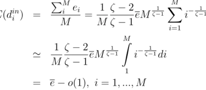
Notice also that the tail parameter only controls the shape of the outdegree distribution - how fat-tailed the distribution will be - but not the average indegree, which is a free parameter, e. That is, it is possible to show that, under parameterization (12), the average weight,

PM

i=1ei

M 'e; .by approximating a …nite sum with an integral thus:

E(din_i ) = PM i ei M = 1 M 2 1eM 1 1 M X i=1 i 11 ' 1 M 2 1eM 1 1 M Z 1 i 11di = e o(1); i= 1; :::; M

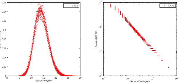
Figure 5 below plots the_A(M; e; ) model-based equivalent of Figures 3 and 4, the inde-gree density and the outdeinde-gree CCDF. It presents the sectoral demand-supply side breakdown for thirty A matrices drawn at random from a family of intersectoral digraphs, _A(M; e; )

where I have picked the following parametrization: M is given by a 500 sector economy, where the average number of inputs needed per sector, e; is set at 15; and the parameter controlling heterogeneity of sectors along the supply side, , is set at 2:1. This parameteri-zation is based on the corresponding objects computed from the B.E.A. detailed input-use matrices in Section 2.

18_{This is adeterministicsequence with power-law like (or scaling) behavior in that it gives a …nite sequence} of real numbers,E(dout

1 ) E(dout2 ) ::: E(dMout), such that i=c[E(douti )] '

where c is a constant and

'is called the scaling index. See Li et al (2006) for a useful discussion on scaling sequences vs. power law distributions.

0 5 10 15 20 25 30 0 0.02 0.04 0.06 0.08 0.1 0.12 0.14 0.16

Sec tor Indegree

E mp ir ic a l D e n s ity 100 101 102 103 10-3 10-2 10-1 100

Sec toral Outdegree

E mp ir ic a l C C D F ζ =2.1 ζ =2.1

Figure 5: Empirical indegree density (l.h.s.) and outdegree CCDF (r.h.s.) for 30 intersectoral trade structures drawn at random from _A(M; e; ) for M = 500, e= 15,

= 2:1:

While individual realizations of A are random objects, thus di¤ering in the exact place-ment of zeros, the indegree and outdegree sequences implied by each realization of the in-tersectoral network yield similar patterns. In other words, row and column sums will not di¤er much across realizations. By design, each realization of_A(M; e; );retains the features noted in Section 2: homogeneity along the demand side - sectoral indegrees concentrate along the speci…ed average degree, e - and heterogeneity along the supply side, where the number of sectors any given sector supplies can di¤er by orders of magnitude. Namely, the outdegree sequences implied by realizations ofAdisplay fat-tails in the form of a power law-as instructed by De…nition 6.

Given a realization of A(GP L_{) and a sequence}

f jgMi=1 I can again resort to Lemma 1

to form the corresponding input-use matrix (GP L_{) . However, some care is needed in}

applying the Lemma, as realizations of Aare now random objects. In particular, recall that the Lemma requires that the indegree, din

i , is strictly positive for all sectors i= 1; :::; M in

order for(I (GP L₎₎ 1 _{to be well de…ned:The following Lemma gives the probability that}

this is indeed the case under the data generating process _A(M; e; ). Lemma 2 Fix a triplet of parameters (M; e; ). Let _fdin₁ ; :::; din

Mg denote the sampled

in-degree sequence, associated to a realization of A(GP L_{) under the data generating process}

A(M; e; ). Then, with probability 1 M

j=1 1

ej

M M

; all elements of the indegree se-quence _fdin

1 ; :::; d in

Thus, and noticing that given a triplet (M; e; ); I can compute the weight sequence {ejgMj=1, I can always compute this probability. For example, for the data generating process

A(500;15;2:1) considered above, the probability that (I (G)) 1 exists is 0.996. More generally, for a …xedM, and given the statement in De…nition 6, the larger is their expected indegree, the smaller is the probability that I sample sectors demanding no intermediate inputs. Alternatively, …xing M and e, the smaller is the higher is this probability since the largest elements of the weight sequence will be closer to M (thus rendering the product term closer to zero). With this technical proviso in mind, I now turn to derive analytical expressions for aggregate volatility as a function of the network structure of intersectoral trade under three di¤erent cases: complete, star and power law intersectoral networks.

3.3

Volatility Decay in Sectoral Networks

In this section I return to the static multisector setup put forth in Section 3.1 and show how the structure of intersectoral linkages in‡uences the volatility of aggregate output. For analyzing the latter, and keeping in line with the literature (see Horvath, 1998, or Dupor, 1999), I take the variance of average log output

2 Y E "PM i=1(yi i) M #2 (15)

as the aggregate volatility statistic. Note that PM_i=1(yi i) is the sum of log sectoral

output (demeaned). Dividing this by the number of sectors gives a log-linear approximation to the more obvious aggregate statistic, the log of total output. The di¢ culty with the latter is that it involves a nonlinear function of the vector of shocks. The average of log sectoral output can therefore be taken as the log-linearization of this function. Using this aggregate statistic will allow me to compare my results directly with those in Horvath (1998) and Dupor (1999)19_.

Using the tools developed in the previous subsection in tandem with Lemma 1, I can now represent the input-use matrix, , as a function of the network of intersectoral linkages, (G), and thus make explicit the link between the latter and aggregate volatility, 2Y( (G)):

Propo-19_{In subsequent work within the same multisector setup presented, Acemoglu et al (2010), show that if we} assume i) _j = for allj, ii) j = 1=M for allj and iii) premultiply the household’s utility function by an

appropriate normalization constant, then aggregate real value added is given by _M(I ) 10". Notice that this is proportional to PM i=1(yi i) M = 1 M(I ) 1 0

". Thus, under these assumptions, the aggregate statistic

2

sition 1 below gives an expression for this statistic in complete network settings, 2

Y( (GC)

versus that obtained with N star networks, 2

Y( (GS)):

Proposition 1 Assume that the share of material inputs, _j = ;and that sectoral volatility

2

j = 2 for all sectorsj = 1; :::; M:Consider the equilibrium of a static multisector economy

(8) where the input-use matrix, ; is given by (GC_{)or by (G}S_{). In either case, (I )} 1

is given by

(I ) 1 =I+

1 1

0

M

where is an M 1 vector with typical element _Pdouti M

i=1douti

and 1M is the unit vector of

dimension M 1. Further, aggregate volatility, 2

Y is given by: 2 Y( (G C_{)) =} 1 1 2 ₂ M (16)

for any complete network of sectoral linkages; and

2 Y( (GS)) = N M + 2 1 2 M + 1 2 2 N (17)

for any N-star network of sectoral linkages.

Notice that with the additional assumptions imposed in the proposition, sectoral tech-nologies in these economies are symmetrical in all respects except, possibly, that some supply to more sectors than others. This is borne out in the expressions for aggregate volatility: they depend only on the share of material inputs, ; sectoral volatility, 2, and the number of e¤ective input suppliers in each case, M or N. The …rst two e¤ects are standard. Thus, the higher the share of material inputs in production the more aggregate volatility will be a¤ected by disturbances working through the input-output network20_{. Similarly, greater} sectoral volatility translates mechanically into heightened volatility in aggregates.

Of interest to this paper is the dependence of aggregate volatility on the number of sectors. Thus, the expression for complete intersectoral structures of input trade is a particular case of the results in Dupor (1999): aggregate volatility scales with 1=M. To understand how e¤ective the shock diversi…cation argument is in this case notice the following: holding sectoral productivity variance …xed as I move from a …ve sector economy to a …ve hundred sector economy, aggregate volatility will be a hundred times smaller. From this, Dupor 20_{This multiplier e¤ect of(1=1 ) on aggregates is a standard feature of multisector economies; see for} example the discussion in Jones (2010a, 2010b)

(1999) concludes that the input-output matrix provides a poor propagation mechanism for independent sectoral shocks.

The result forN star sectoral networks o¤ers a di¤erent, if somewhat predictable, view. In an economy where the e¤ective number of input suppliers is small, the law of large numbers will be postponed relative to that of Dupor (1999): aggregate volatility now scales with

1=N, the slowest decaying term in expression (29) 21_{. This is Horvath’s (1998) argument:} limited sectoral interaction yields greater aggregate volatility from sector speci…c shocks. The di¢ culty with this result is that the modeler is now left to specify, for each M;what is the number of input suppliers in an economy; N. If, as Horvath (1998) argues, that N is of orderpM, this would yield a ten fold decrease in aggregate variability as we move from …ve to …ve hundred sectors.

I now show that when we abandon these two extreme cases and instead consider more realistic power law sectoral networks - (GP L_{)- aggregate volatility decays withM ;where}

2 (0;1] depending on the speci…c value of the tail parameter in the power law. Thus I show that the power law speci…cation subsumes the two extreme cases above.

Proposition 2 Assume that the share of material inputs, _j = ;and that sectoral volatility

2

j = 2 for all sectorsj = 1; :::; M:Consider the equilibrium of a static multisector economy

(8) where is given by (GP L)for any A(GP L)sampled from the family of input-use graphs

A(M; e; ):Then, with probability 1 M_j=1 1 ej

M M

; I (GP L) 1 is well de…ned and given by:

I (GP L) 1 =I+

1 e1

0

M +

where e is an M 1 vector with typical element E(douti )

PM

i=1E(douti )

and is an M M random matrix with zero column sums. Further, whenever this is the case; 2

Y( (GP L)) bounded below by: (1 o(1)) ₁ 2 1( ) 2 M if >3 or (1 o(1)) ₁ 2 2( ) _M1 2 4 1 2 _if 2(2;3) where 1( ) = ( 2)2 ( 1)( 3) and 2( ) = ( 2)2

( 1)(3 ); positive constants given a .

To interpret the Proposition consider the following thought experiment. Fix a number of sectors, M; and de…ne a typical production technology by setting the average number of 21_{As it should be, the two expressions in Proposition 1 will be equal forN =M. Notice that ifN is …xed} for anyM the law of large numbers breaks down completely.

inputs(e) a sector needs, in order to produce its output. Now entertain two di¤erent values of the tail parameter governing heterogeneity across sectors in their role as input suppliers,

1 and 2 such that 2 < 1 < 3 < 2. What this yields are two economies where sectoral

production technologies di¤er in their degree of diversi…cation. Thus 1 economies will be

less diversi…ed in that more mass at the tail implies that a greater number of sectors rely on the same general purpose inputs. Conversely, ₂ economies, by having more mass at the center of the distribution of input supply links, will be more diversi…ed: there will be a smaller number of hub-like sectors connecting all sectors in the economy and a greater number of specialized input suppliers, each supplying inputs to a smaller fraction of sectors. The proposition states that the scaling of the aggregate volatility statistic with M is dependent which on region of the parameter space is set, or alternatively, how diversi…ed is the structure of intersectoral linkages in the economy. Thus, for thin tailed distributions of sectoral outdegrees > 3, aggregate volatility scales with the usual term of order O(1=M). This means that the discussion regarding the decay rate in the special case of complete network structures assumed by Dupor, applies also to the current context. Intuitively, in economies with a large number of sectors that do not di¤er much in their role as input suppliers, aggregate volatility will be negligible.

However, once we consider the fat-tailed region for ₂(2;3)the decay behavior is altered: the aggregate volatility statistic now decays with M at a rate that is lowered signi…cantly as we consider input use matrices from more heterogeneous outdegree economies:Namely, Proposition 2 yields an analytical expression where the rate of decay in the volatility of aggregate output depends negatively on the degree of fat-tailness in the distribution of sectoral input-supply links. To see this notice that for ₂(2;3); the term in the expression decays with M where 2 ₁4 ₂ (0;1) Namely, as approaches its lower bound of

2; aggregate volatility, 2

Y( (GP L)) will converge to zero arbitrarily slower. Taking, for

example, the average value of of 2.1. in Section 2, yields a much slower decay of orderp6M

or 2Y( ) _ 2 6

p

M. To have an idea of the magnitudes involved, this means that as I move

from, say, a …ve sector economy to a …ve hundred sector economy I expect to …nd only a

two-fold decrease in aggregate volatility. Thus, strong heterogeneity across input-supplying sectors opens the possibility of generating non-negligible aggregate ‡uctuations even in large scale multi-sectoral contexts22_.

In short higher values of yield greater technological diversi…cation: sectoral technologies 22_{Notice also that Horvath (1998) conjecture of a}p_{M decay in aggregate volatility is obtained by …xing} at a very particular point: = 2:333:

are relatively more reliant on specialized input-suppliers and less so on common, general purpose, inputs. Therefore, greater diversi…cation in the form of less reliance on common inputs will yield only loosely coupled technologies and, as a result, lower aggregate volatility. Less diversi…cation induces strongly coupled technologies and thus a stronger propagation mechanism23_{. The next section will show that this intuition carries through when we move} to dynamic multi-sector settings.

4

Dynamic Multi-Sector Economies

This section recalls a baseline dynamic multi-sectoral model, as introduced in Horvath (1998), Dupor (1999) and Foerster, Sarte and Watson (2008). This is a multi-sector version of a one-sector Brock-Mirman stochastic economy. Following Horvath (1998) and Dupor (1999), I show that, for a particular case where it is possible to solve for the planner’s solution analytically, the results derived in the previous section extend to a dynamic setting. I then return to the general setup and present some quantitative explorations.

4.1

General Setup

A representative agent maximizes her expected discounted log utility from in…nite vector valued sequences of consumption ofM distinct goods and leisure.

E0 1 X t=0 t " _M X j=1 log(Cjt) Ljt # (18)

where is a time discount parameter in the (0;1) interval, Ljt is labor devoted to the

production of the jth _{good at time t. Expectation is taken at time zero with respect to the}

in…nite sequences of productivity levels in each sector, the only source of uncertainty in the economy.

The production technology for each good j = 1; :::; M combines sector-speci…c capital, labor and intermediate goods in a Cobb-Douglas fashion:

Yjt =ZjtK j jt L 'j jt M Y i=1 M ij ijt (19)

23_{See Simon and Ando (1961) for a distant forerunner in analyzing the implications of loose vs. strong} coupling across units.

whereKjt;andZjt are, respectively, timet; sectorj; value of sector speci…c capital stock

and its (neutral) productivity level. Mijt gives the amount of good i used in sector j in

period t. Further, de…ne

j = M X

i=1

ij

with _ij denoting the cost-share of input from sector i in the total expenditure on inter-mediate inputs for sector j (allowed to take the value of zero). Again I can arrange the cost shares in a M M input-use matrix, . Constant returns to scale are assumed to hold at the sectoral level such that:

j +'j + M X

i=1

ij = 1;8j (20)

It’s assumed that sector-speci…c capital depreciates at rate :

Kjt+1 =Ijt+ (1 )Kjt (21)

where Ijt is the amount of investment in sector j0s capital at time t. Note that due to

the sector-speci…c nature of capital, the sectoral resource constraints are given by:

Yjt =Cjt+Kjt+1 (1 )Kjt+

M X

i=1

Mjit (22)

Finally, I further assume that the log of sector speci…c productivity follows a random walk

ln(Zjt) = ln(Zjt 1) +"jt; "jt sN(0; 2) (23)

where the sectoral innovations are assumed to be i.i.d. both in the cross section and across time.

De…nition 7 The Social Planner’s problem is to choose sequences of sector speci…c capital

fKjt+1gj;t, intermediate inputs fMijtgi;j;t labor fLjtgj;t and consumption allocationsfCjtgj;t

such that, given a vector of time zero capital stocks _fKj0gj and a sequence of sectoral

pro-ductivity levels _fZjtgt drawn from (23), the following hold true:

i)_fCjt; Ljtgj;t maximizes the representative consumer expected lifetime utility given by

(18)

ii) the sectoral resource constraint (22) is satis…ed, sector by sector, for all time periods, where Yjt is given by (19).

iii) the labor allocation across sectors is feasible, PM_j=1Ljt =L for all t; where L is the

time endowment of the household

As Foerster, Sarte and Watson (2008) show, the characterization of the deterministic steady state of this model is analytically tractable and a log-linearization around that steady state yields:

yt+1 = yt+ "t+1+ "t (24)

where yt+1is anM 1vector of percentage deviations around the sectoral steady state,

"t+1 is a vector of sectoral productivity shocks and ; and are M M matrices that

depend on model parameters only.

4.2

Analytical Solutions in a Special Case

I now take a special case of the setup above, where explicit analytical solutions are available. In particular, I follow Horvath (1998) and Dupor (1999) and assume that there is no labor ('_j = 0 for all j) and that sector-speci…c capital depreciates fully ( = 1). Under these· assumptions, Dupor (1993, fn.3) and Foerster, Sarte and Watson (2008) show that the planner’s problem now yields an analytical solution given by the …rst order autoregression:

yt+1 = (I ) 10 d yt+ (I ) 10"t+1 (25)

where dis aM M diagonal matrix with the vector of capital shares on its diagonal.

As in the simple static setup of Section 3, it is the Leontie¤ inverse (I ) 1 _{that mediates}

the propagation of independent technology shocks at the sectoral level. Now, in order to characterize the second moment properties of this economy, I study the spectral density function for sectoral output growth induced by expression (25) above. This is possible since, under the assumptions made here, the_f ytgt sequence given by (25) is stationary and thus

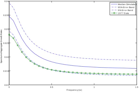
admits an in…nite moving average representation which, in turn, implies a frequency domain representation. In particular, under the assumptions made above, it is easy to show that the population spectrum for sectoral output growth, y_t;at frequency ! is given by

S y(!; ) : = 2 (2 )(I de i! 0₎ 1_(I dei! ) 1 (26)

Furthermore, given anM 1vectorwof aggregation weights, the spectrum for aggregate output growth at frequency! is given by

The spectral density function is a useful object in that it provides a complete charac-terization of the autocovariance function for average sectoral output growth. Notice that by setting the elements of w to be equal and given by 1=M, S(!; ) is gives the dynamic counterpart to the aggregate statistic (15) of the static model of Section 3

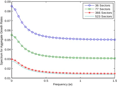
I now turn to characterizing the decay of the univariate spectral density expression (27) with the number of sectors for the case of power law sectoral linkages (GP L_).

Proposition 3 Assume that the share of material inputs, j = for all sectorsj = 1; :::; M:

Consider the population spectrum for sectoral output growth S y(!; )(26) where is given

by (GP L_{) for any A(G}P L_{) sampled from the family of input-use graphs A(M; e; ): Then,}

with probability 1 M j=1 1

ej

M M

; I (GP L₎ 1 _{is well de…ned: Whenever this is the}

case and for aggregation weights w = (1=M)1M; the spectral density for aggregate output

growth S(!; (GP L_{)), is bounded below by :}

1 2 a(!) b(!) (b(!) 2₎ 2 M + (1 o(1)) 2 1( ) 2 M if >3 and 1 2 a(!) b(!) " (b(!) 2) 2 M + (1 o(1)) 2 2( ) 1 M 2 4 1 2 # if ₂(2;3) where a(!) = _{(1 e}i! ₎₍₁1 _e i! ₎,b(!) = (1 e i!_{)(1 e} i!_); 1( ) = ( 2)2 ( 1)( 3) and 2( ) = ( 2) 2 ( 1)(3 ).

As in Proposition 2, the expression for the volatility of aggregates di¤ers according to the tail parameter governing heterogeneity across sectors in their role as input suppliers. Thus for > 3, i.e. thin tail distributions, or diversi…ed economies, the expression again recovers the strong diversi…cation of shocks argument given in Dupor. Volatility in aggregate variables decays at rateM as we expand the number of sectors, yielding negligible aggregate volatility for any moderate level of disaggregation. Conversely, for economies where large input-supplying hubs form the basis for input trade ‡ows, this decay rate is slowed down arbitrarily as approaches its lower bound. The more every sectoral technology in an economy relies on the same few key inputs the slower the law of large numbers applies.

However, as the Proposition makes clear, this scaling now extends to the autocovariance function of output growth. In particular, exactly the same decay description applies for all frequencies of the spectral density of aggregate output growth. This means that, for any input-use matrix based on sectoral networks given by _A(M; e; ), there is a link between