Learning-by-exporting in Korean Manufacturing: A Plant-level Analysis

ERIA-DP-2009-04

ERIA Discussion Paper Series

Learning-by-exporting

in Korean Manufacturing:

A Plant-level Analysis

Chin Hee HAHN*

Chang-Gyun PARK

Korea Development Institute, Korea

†

College of Business Administration, Chung-Ang University, Korea

March 2009

Abstract: The paper analyzes whether firms that start exporting become more productive utilizing recently developed sample matching procedures to control the problems from self-selection into the export market. We use plant level panel data on Korean manufacturing sector from 1990 to 1998. We find clear and robust empirical evidence in favor of the learning-by-exporting effect; total factor productivity differentials between exporters and their domestic counterparts arises and widens during several years after export market entry. We also find that the effect is more pronounced for firms that have higher skill-intensity, higher share of exports in production, and are small in size. Overall, the evidence suggests that exporting is one important channel through which domestic firms acquire accesses to advanced knowledge and better technology. Also, the stronger learning-by-doing effect for firms with higher skill-intensity seems to support the view that “absorptive capacity” matters to receive knowledge spillovers from exporting activity.

Keywords: Learning-by-exporting, Productivity, Propensity score matching.

JEL Classification: F14, O12, O19.

*

Chin Hee Hahn: Senior Research Fellow, Korea Development Institute; [email protected].

†

Chang-Gyun Park: Assistant Professor, College of Business Administration, Chung-Ang University; [email protected].

1

1. Introduction

One of the most frequently asked question in trade and growth literature is whether and how international trade or openness of trading regime promotes productivity growth of countries. Although numerous studies, both theoretical and empirical, have been conducted on this issue, there seems to be no clear consensus yet. Recently, a growing number of studies have started to utilize firm or plant level data and re-examined this issue, particularly focusing on exporting as a channel of international technology diffusion or knowledge spillover. One empirical regularity emerging from these studies is that exporters are more productive than non-exporters. The positive correlation between exporting and productivity in cross-sectional context, however, provides little useful information on the direction of causality. On one hand, this could reflect self-selection into export market: only productive firms can expect to recoup the sunk entry cost of entering into the export market and join the export market. In this case, the causality runs from productivity to exporting. On the other hand, it is also plausible that the positive correlation between exporting and productivity reflects learning-by-exporting effect: firms that become exporters could gain new knowledge and expertise after entering export market and improve their productivity relative to average player in the same industry. The self-selection hypothesis is supported by most studies, but the evidence on learning-by-exporting seems less clear-cut (Tybout 2000).

This paper examines the exporting-productivity nexus utilizing the plant level panel data on Korean manufacturing sector (Survey of Mining and Manufacturing, SMM henceforth) from 1990 to 1998. The main question to be addressed is whether

2

exporting activity improves productivity performance of plants. The emphasis on learning-by-exporting in the paper stems from the recognition that it is the area where existing literature presents mixed empirical results and, nevertheless, whether or not the learning-by-exporting effect exists has an important implication on the formulation of appropriate policy stance toward “openness”. As discussed by Bernard and Jensen (1999a), if the gains do accrue to firms once they become exporters, then the appropriate policy interventions would be those that reduce barriers to entering foreign markets including macroeconomic trade policies to promote openness to trade and microeconomic policies to reduce entry costs, such as export assistance, information programs, joint marketing efforts, and trade credits. On the other hand, if there are no post-entry rewards from exporting, these policies designed to increase the numbers of exporters are more likely to end up wasting resources.4

Furthermore, this paper attempts to clarify the conditions, if at all, under which the learning-by-exporting may or may not take place, utilizing information on some plant or industry characteristics. As plantcharacteristics, we consider skill-intensity, export propensity, plant size, and R&D intensity. Most existing studies utilized information only on whether a plant exports or not and focused on the existence of learning-by-exporting effect. However, it is plausible that the degree of learning-by-learning-by-exporting could be related to, for example, how important exporting activity is to the plant involved, in as much as learning-by-exporting arises through interactions with foreign buyers which requires costly resources. Thus, we examine whether plants with higher export propensity enjoys more benefits of learning-by-exporting. Meanwhile, if knowledge spillovers from exporting activities require domestic “absorptive capacity”,

4

3

then we could expect that plants with higher absorptive capacity will exhibit stronger learning-by-exporting. We use the skill-intensity of plants as a proxy for the domestic absorptive capacity.

We also examine whether the destination of exports matter in learning-by-exporting a là Loecker (2007). He shows that the degree of learning-by-learning-by-exporting depends on destination of exports, using plant level information on the export destination in Slovenian manufacturing. The analysis is based on the presumption that learning-by-exporting effect will be stronger for plants that start exporting to more advanced countries. In case of Korea, however, the plant level information about the export destination is not available. So, we examine instead whether plants in industries with higher share of exports to advanced countries tend to exhibit stronger learning-by-exporting.

Examining these issues in the Korean case is particularly important in several respects. Above all, as well recognized, Korea is one of the few success countries that has narrowed the income gap with advanced countries by adopting an outward-oriented trade strategy.5

There are some empirical studies that scrutinize the causal relationship between So, examining and clarifying the openness-productivity nexus in the Korean case could provide valuable lessons on other developing countries that hope to catch-up with advanced countries. Furthermore, Korea is a country with large external exposure in trade that still needs to make a transition toward a fully developed country. Thus, in so far as learning-by-exporting, if it exists, reflects trade-related uni-directional knowledge spillovers from advanced to less-advanced countries, Korea is the appropriate place to examine these issues.

5

4

exporting and productivity. Most studies report that exporters are more productive than non-exporters before they start to export, suggesting that cross-sectional correlation between exporting and productivity partly reflects a self-selection effect. For example, Clerides, Lach and Tybout (1998) find very little evidence that previous exposure to exporting activities improves performance, using the plant-level panel data from Colombia, Mexico, and Morocco. Similar results are reported by Aw, Chung, and Roberts (2000) and Aw, Chen, and Roberts (2001) for Taiwan, Bernard and Jensen (1999b) for U.S. By contrast, the evidence on a learning effect is mixed. Earlier research such as Bernard and Jensen (1999b) find little evidence in favor of learning. They report that new entrants into the export market experience some productivity improvement at around the time of entry, they are skeptical about the existence of strong learning-by-exporting effect. However, several recent studies utilizing more refined empirical technique to deal with self-selection problem such as matched sampling techniques provide some empirical evidence in favor of learning-by-exporting. See Girma, Greenaway, and Kneller (2004) for UK, De Loecker (2007) for Slovenia, and Albornoz and Ercolani (2007) for Argentina.

Related previous studies on Korea include Aw, Chung, and Roberts (2000) and Hahn (2004). Aw, Chung, and Roberts (2000), using plant-level panel data on Korean manufacturing for three years spaced at five-year intervals, does not find evidence in favor of either self-selection or learning-by-exporting. It differs from similar studies on other countries in that even the self-selection hypothesis is not supported. Aw, Chung, and Roberts (2000) argue that Korean government’s investment subsidies tied to exporting activity rendered plant productivity a less useful guide on the decision to export. By contrast, following the methodologies of Bernard and Jensen (1999a,

5

1999b), Hahn (2004) finds some supporting evidence for both selection and learning in Korean manufacturing sector, using annual plant-level panel data from 1990 to 1998. However, Hahn (2004) suffers from the same technical difficulties as Bernard and Jensen (1999a, 1999b) in that the uncontrolled self-selection problem in export market participation may have contaminated the result.

In this paper, we re-examine the learning-by-exporting hypothesis in Korean manufacturing sector controlling for the self-selection in export market participation with a recently developed statistical tool: propensity score matching.

The organization of this paper is as follows. The following section explains the data set and the calculation of plant total factor productivity. Section 3 briefly discusses the estimation strategy to overcome the difficulties arising from self-selection in decision making for export market participation and to obtain a better estimate for the effects of learning-by-exporting. Section 4 discusses our main empirical results and the final section concludes.

2.

Data and Plant Total Factor Productivity

2.1. Data

This paper utilizes the unpublished plant-level census data underlying the Survey of Mining and Manufacturing in Korea. The data set covers all plants with five or more employees in 580 manufacturing industries at KSIC (Korean Standard Industrial Classification) five-digit level. It is an unbalanced panel data with about 69,000 to 97,000 plants for each year from 1990 to 1998. For each year, the amount of exports

6

as well as other variables related to production structure of plants, such as production, shipments, the number of production and non-production workers and the tangible fixed investments, are available. The exports in this data set include direct exports and shipments to other exporters and wholesalers, but do not include shipments for further manufacture.

2.2. Plant Total Factor Productivity

Plant total factor productivity (TFP) is estimated following the chained-multilateral index number approach as developed in Good (1985) and Good, Nadiri, and Sickles (1996). This procedure uses a separate reference point for each cross-section of observations and then chain-links the reference points together over time. The reference point for a given time period is constructed as a hypothetical firm with input shares that equal the arithmetic mean input shares and input levels that equal the geometric mean of the inputs over all cross-section observations. Thus, output, inputs, and productivity level of each firm in each year is measured relative to the hypothetical firm at the base time period. This approach allows us to make transitive comparisons of productivity levels among observations in panel data set.6

6

Good, Nadiri, and Sickles (1996) summarize the usefulness of chaining multilateral productivity indices. While the chaining approach of Tornqvist-Theil index, the discrete Divisia, is useful in time series applications where input shares might change over time, it has severe limitations in cross-section or panel data framework where there is no obvious way of sequencing the observations. To the contrary, the hypothetical firm approach allows us to make transitive comparisons among cross-section data, while it has an undesirable property of sample dependency. The desirable properties of both chaining approach and the hypothetical firm approach can be incorporated into a single index by chained-multilateral index number approach.

Specifically, the productivity index for firm i at time t in our study is measured in the following way.

7

(

)

(

)

∑

∑

∑

∑

where Y,X, S, and TFP denote output, input, input share, TFP level, respectively, and symbols with an upper bar are corresponding measures for the hypothetical firm. The subscripts τ and n are indices for time and inputs, respectively. The year 1990 is chosen as the base year.

As a measure of output, we use the gross output (production) of each plant in the Survey deflated by the producer price index at disaggregated level. The capital stock used in this paper is the average of the beginning and end of the year book value of capital stock in the Survey deflated by the capital goods deflator. As for labor input,

we use the number of workers, which includes paid employees7

7

Paid employees is the sum of production and non-production workers.

, working proprietors and unpaid family workers. We allowed for the quality differential between production workers and all other types of workers. The labor quality index of the latter was calculated as the ratio of non-production workers’ and production workers’ average wage at each plant, averaged again over the entire plants in a given year. The sum of “major production cost” and “other production cost” reported in the Survey was taken as the measure of intermediate input. Major production cost covers costs arising from materials, parts, fuel, electricity, water, manufactured goods outsourced and maintenance. Other production cost covers expenditures on outsourced services such as advertising, transportation, communication and insurance. The estimated intermediate input was deflated by the intermediate input price index.

8

We assumed constant returns to scale production technology so that the sum of factor elasticities equals to one. Labor and intermediate input elasticities for each plant are measured as average factor cost shares within the same plant-size class in the five-digit industry in a given year. Here, plants are grouped into three size classes according to the number of employees; 5-50, 51-300, and over 300. Thus, the factor elasticities of plants are allowed to vary across industries and plant size classes and over time.

2.3. Definition of Exporters

Following convention in the literature, we define an exporter in a given year as a plant reporting positive amount of exports. Accordingly, non-exporters in a given year are those plants with zero exports. With this definition of exporters, it is possible to classify all plants into five sub-groups: Always, Never, Starters, Stoppers, and Other.8

8

We eliminated plants that switch in and out of the dataset more than twice during the sample period. Thus, we keep only those plants that do not have a split in time series observations. This procedure eliminates about 10 percent of the sample in terms of number of plants.

“Always” is a group of plants that were exporters in the year that they first appear in the data set and never changed their exporting status. Similarly, “Never” is a group of plants that were non-exporters in the year that they first appear in the data set and never switched to exporters. “Starters” includes all plants that were non-exporters in the year that they first appear, but switched to non-exporters in some later year and remained as exporters thereafter. “Stoppers” consists of all plants that were exporters in the year that they first appear, and then switched to non-exporters, never switching back to exporters thereafter. All other plants that switched their exporting status more than twice during the sample period are grouped as “Other”.

9

2.4. A Preliminary Analysis: Performance of Exporters and Non-exporters Table 1 shows the number of exporting plants and average exports as percentage of shipments, or export intensity, for each year during the sample period. Exporting plants accounted for between 11.0 and 15.3 percent of all manufacturing plants. The share of exporting plants rose slightly between 1990 and 1992, but since then steadily declined until 1996. However, with the outbreak of the financial crisis in 1997, the share of exporting plants rose somewhat noticeably to reach 14.8 percent in 1998. The rise in the share of exporting plants can be attributed mostly to the closure of non-exporting plants, rather than increase in the number of non-exporting plants. Note that the increases in the number of exporters in 1997 and 1998 were modest, which are broadly consistent with the severe contraction of domestic demand and huge depreciation of Korean Won associated with the crisis.

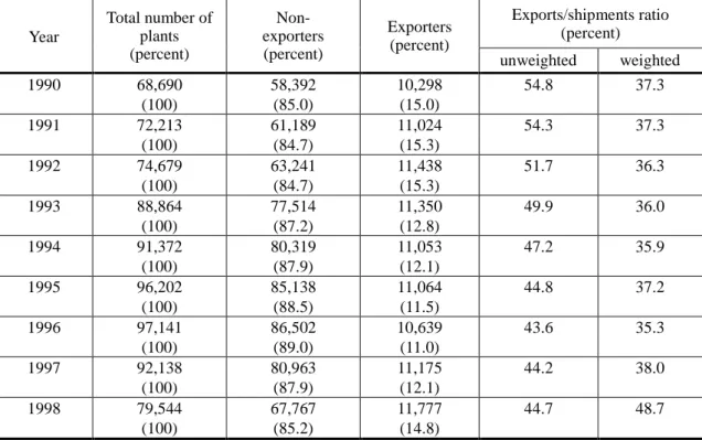
Table 1. Number of Exporters and Export Intensity

Year Total number of plants (percent) Non- exporters (percent) Exporters (percent) Exports/shipments ratio (percent) unweighted weighted 1990 68,690 58,392 10,298 54.8 37.3 (100) (85.0) (15.0) 1991 72,213 61,189 11,024 54.3 37.3 (100) (84.7) (15.3) 1992 74,679 63,241 11,438 51.7 36.3 (100) (84.7) (15.3) 1993 88,864 77,514 11,350 49.9 36.0 (100) (87.2) (12.8) 1994 91,372 80,319 11,053 47.2 35.9 (100) (87.9) (12.1) 1995 96,202 85,138 11,064 44.8 37.2 (100) (88.5) (11.5) 1996 97,141 86,502 10,639 43.6 35.3 (100) (89.0) (11.0) 1997 92,138 80,963 11,175 44.2 38.0 (100) (87.9) (12.1) 1998 79,544 67,767 11,777 44.7 48.7 (100) (85.2) (14.8) Source: Hahn (2004).

10

Consistent with the high export propensity of the Korean economy, the share of exports in shipments at plant level is quite high. During the sample period, the unweighted mean export intensity is between 43.6 and 54.8 percent, declining from 1990 to 1996 but rising with the onset of the crisis in 1997. The average export intensity weighted by shipment shows a similar pattern, with generally lower figures than the unweighted average, suggesting that smaller exporting plants have a higher export intensity.

It is a well-established fact that exporters are better than non-exporters by various performance standards. Table 2 compares various plant attributes between exporters and non-exporters for three selected years. First, exporters are on average much larger in the number of workers and shipments than non-exporters. The differential in shipments is more substantial than that in the number of workers. So, the average labor productivity of exporters measured by either production per worker or value added per worker is higher than that of non-exporters. Compared with the cases of value added, the differential in production per worker between exporters and non-exporters is more pronounced. This might reflect a more intermediate-intensive production structure of exporters relative to non-exporters. Although exporters show both higher capital-labor ratio and a higher share of non-production workers in employment than non-exporters, they do not fully account for the differences in labor productivity. As a consequence, total factor productivity levels of exporting plants are, on average, higher than those plants that produce for the domestic market only. Some differences in the total factor productivity may be attributed to the differences in R&D intensity. Note that, controlling forthe size of shipments, exporters spent about twice as much on R&D as non-exporters. From a worker’s point of view, exporters

11

had more desirable attributes than non-exporters. That is, the average wage of exporters is higher than that of non-exporters. Although both a production worker’s wage and a production worker’s wage are higher in exporters than in non-exporters, the differential in the non-production worker’s wage is more pronounced.

Table 2. Performance Characteristics of Exporters vs. Non-exporters

1990 1994 1998 exporters non-exporters exporters non- exporters exporters non- exporters Employment (person) 153.6 24.5 119.4 20.0 95.1 17.8 Shipments (million won) 11,505.5 957.0 17,637.1 1,260.3 25,896.8 1,773.8 production per worker

(million won) 50.5 26.8 92.4 47.0 155.0 74.2 value-added per worker

(million won) 16.5 11.3 31.0 20.4 51.3 29.6 TFP 0.005 -0.046 0.183 0.138 0.329 0.209 capital per worker

(million won) 16.8 11.9 36.0 21.9 64.6 36.7 non-production worker/ total employment (percent) 24.9 17.1 27.5 17.5 29.6 19.2 average wage (million won) 5.7 5.1 10.3 9.2 13.7 11.5 Average production wage

(million won) 5.5 5.1 10.0 9.2 13.1 11.4 average non-production

wage (million won) 6.8 5.3 11.6 9.4 15.6 12.4 R&D/shipments

(percent) - - 1.2 0.6 1.4 0.6

12

3. Empirical Strategy: Propensity Score Matching

It is now well-recognized in the literature that the decision to become an exporter is not a random event but a result of deliberate choice, requiring special efforts to correctly identify the true effect of becoming an exporter on its productivity (Loecker 2007, Albornoz and Ercolani 2007). The participation decision in the export market is likely to be correlated with the stochastic disturbance terms in the data generating process for a firm’s productivity, so that the traditional simple mean difference test on productivity differences between exporters and non-exporters does not provide the correct answer. The matching method has been gaining popularity among applied researchers since it is viewed as a promising analytical tool with which we can cope with statistical problems stemming from an endogenous participation decision.

The underlying motivation for the matching method is to reproduce the treatment group (exporters) out of the non-treated (non-exporters), so that we can reproduce the experiment conditions in a non-experimental setting. Matched samples enable us to construct a group of pseudo-observations containing the missing information on the treated outcomes had they not been treated by paring each participant with members of the non-treated group. The crucial assumption is that, conditional on some observable characteristics of the participants, the potential outcome in the absence of the treatment is independent of the participation status.

i i i d X

y0 ⊥ ₍₂₎

where yi0 is the potential outcome in the absence of the treatment, di is the dummy

13

idea of matching is to construct a sample analog of a counter factual control group by identifying the members of a non-participating group that possess conditioning variables as close to those of treatment group as possible. In practice, it is very difficult to construct a control group that satisfies the condition in (2), especially when the dimension of the conditioning vector Xi is high.

Rosenbaum and Rubin (1983) propose a clever way to overcome the curse of dimensionality in the traditional matching method. Suppose that the conditional

probability of firm i’s becoming an exporter can be specified as a function of

observable characteristics of the firm before the participation;

( )

[

]

(

)

p =Pr =1 = (3)

Rosenbaum and Rubin (1983) call the probability function in (3) propensity score and show that if the conditional independence assumption in (2) is satisfied it is also valid for p

( )

( )

i d p X

y0 ⊥ ₍₄₎

We have replaced the multi-dimensional vector with a one-dimensional variable containing the same information contents so that the highly complicated matching problem in (2) is reduced to a simple single dimensional one in (4).

One can define the average treatment effect on the treated (ATT) as;

[

]

[

[

( )

]

]

( )

[

]

[

( )

]

[

]

14

firm i decided not to participate in an export market and y1i is the observable

outcome for participating firm i. Note that ATT is not the measure for the effect of exporting on all firms but on firms that start to export.

Since yi0 is not observable, the definition (5) is not operational. Given that the

unconfoundedness condition under propensity score (4) is satisfied and the propensity score (3) is known, the following definition is equivalent to (5).

[

]

[

[

( )

]

[

( )

]

]

E

ATT = 1 − 0 =1 = 1 =1, − 0 =0, (6)

Since both yi0 and

1

i

y are observable in (6), one can construct an estimator for ATT by constructing its sample analog.

As the first step, we estimate the probability function in (3) with the following probit specification.

(

)

∫

Log of total factor productivity, log of the number of workers employed, log of capital per worker, 9 yearly dummies, and 10 industry dummies are included in the conditioning vectorXi. As for conditioning variables, we use the values from one

year before the firm starts to export in order to account for the time difference between decision to participate and actual participation.

Based on estimated version of (7), one can calculate propensity score for all observations, participants and non-participants. Let T be the set of treated (exporting) units and C the set of control (non-exporting) units, respectively, and denote by C

( )

15

the set of control units matched to the treated unit i with an estimated value of propensity score ofpi. Then, we pick the set of nearest-neighbor matching as;

( )

j p p

i

C =min − (8)

Denote the number of controls matched with a treated unit i∈T by NiC and define

the weight C

i ij

N

w = 1 _if j∈C

( )

∑

∑

where y1i,t is the observed value on firm i in the treatment group at time t and

0 ,t j

y the observed value on firm j in the matched control group for firm i at time t. Moreover, one can easily show that the variance of the estimator in (9) is given by;

(

)

( )

_{( )}

( )

( )

∑ ∑

One can estimate an asymptotically consistent estimator for (10) by replacing two variance terms for the treatment and control groups with corresponding sample analogs. We use two different versions of the propensity score matching procedure written in STATA language; attn.ado explained in Becker and Ichino (2002) (BI, hereafter) and psmatch2.ado provided by Leuven and Sianesi (2003) (LS, hereafter). The two procedures follow an identical approach in estimating propensity score and constructing the control group, except for the fact that the former tries to verify the

16

unconfoundedness condition in the sample by dividing the entire region of estimated propensity scores into several blocks and construct the matched control group within the block to which the treated observation belongs.

In order to allow for the possibility that the effect of learning by exporting works at different intensities depending on a firm’s characteristics and industry, we divide the entire sample into several categories according to plant or industry characteristics, such as the export intensity of plants, skill intensity of plants, plant size measured by the number of workers, R&D intensity of plants, and export destination of industries. We measure the average treatment effect of the treated for each sub-sample.

4. Empirical Results: Learning-by-exporting Effects

4.1. Starter vs Non-exporter

Table 3 reports the estimated productivity gain from participating in an export market when heterogeneity in treatment effect is not taken into account. The estimated coefficients indicate percentage productivity differentials between plants that start exporting and their domestic counter-parts s years after entering the export market. We report results from the two different versions of propensity score matching procedure, BI and LS.

17

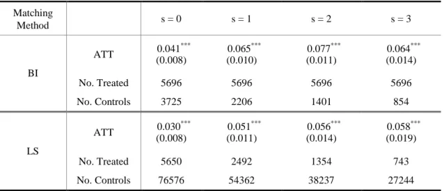
Table 3. Average Productivity Gain of Exporters Matching Method s = 0 s = 1 s = 2 s = 3 BI ATT 0.041 *** (0.008) 0.065*** (0.010) 0.077*** (0.011) 0.064*** (0.014) No. Treated 5696 5696 5696 5696 No. Controls 3725 2206 1401 854 LS ATT 0.030 *** (0.008) 0.051*** (0.011) 0.056*** (0.014) 0.058*** (0.019) No. Treated 5650 2492 1354 743 No. Controls 76576 54362 38237 27244

First and foremost, all estimated coefficients are positive and highly significant, suggesting the existence of a learning-by-exporting effect. This is quite a surprising finding considering the fact that most previous studies were skeptical about the existence of the learning-by-exporting effect. Second, productivity gain for starters begins to materialize immediately after entering the export market, and the productivity gap between the starters and non-exporters9

9

Non-exporters correspond to the “never” group in our earlier definition.

widens further as time passes, although at a decelerating pace. Third, it seems that the choice of procedures in constructing the control group does not yield any material differences in the final result, not only qualitatively but also qualitatively. The estimated coefficients from BI procedure indicate that starters become about 4.1 percent more productive in the year of entry. Over the following years, productivity gain for starters fluctuates between 6.4 and 7.7 percentage points. Thus, it is suggested that entering the export market has a permanent effect on productivity level, especially during the first several years after entry. In other words, export market entry has a temporary effect on productivity growth especially during the first few years after entry.

18

4.2. Sub-group Estimation: Plant Characteristics

In order to allow for a differential treatment effect depending on plant characteristics, we divided our sample into three sub-groups according to various features such as an exports-production ratio, the skill intensity, plant size measured by the number of workers, and R&D-production ratio. Then we apply the matching estimators discussed in Section 3 and estimate the learning-by-exporting effect separately for each sub-group. Based on BI procedure10

10

Estimation results based on LS procedure are reported in the appendix.

, we report the estimated productivity gains for starters in each sub-group in Table 4.

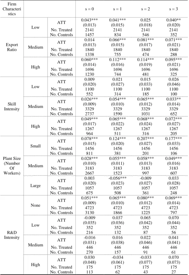
First, the estimated coefficients are generally larger and more significant for plants with higher exports-production ratio. For example, in the group of low export intensity with exports-production ratio of less than 10%, starters become more productive, between 2.5 and 4.1 percent during the three years after the participation. By contrast, in the group of high export intensity with an exports-production ratio greater than 50%, productivity gains for starters are between 9.5 and 11.4 percent for the same time span. In the earlier section, we argued that if the estimated effect of learning-by-exporting indeed captures the beneficial consequences of learning activities associated with exporting, then the effect is likely to be stronger for plants with higher exports-output ratios; if learning-by-exporting arises from contact with foreign buyers and foreign markets, which require costly resources, then firms for whom exporting is their major activity are likely to be more heavily exposed to foreign contact and experience productivity gain. The results for sub-groups with different export intensities are very consistent with this hypothesis.

19

Table 4. Average Productivity Gain of Starters by Firm Characteristics: BI Procedure Firm Characteri stics s = 0 s = 1 s = 2 s = 3 Export Ratio Low ATT 0.043*** (0.013) 0.041*** (0.015) 0.025 (0.018) 0.040** (0.020) No. Treated 2141 2141 2141 2141 No. Controls 1457 834 546 352 Medium ATT 0.014 (0.013) 0.066*** (0.015) 0.081*** (0.017) 0.071*** (0.021) No. Treated 1840 1840 1840 1840 No. Controls 1338 755 474 288 High ATT 0.060*** (0.014) 0.112*** (0.016) 0.114*** (0.019) 0.095*** (0.021) No. Treated 1696 1696 1696 1696 No. Controls 1230 744 481 325 Skill Intensity Low ATT 0.009 (0.020) 0.021 (0.027) 0.015 (0.033) 0.026 (0.046) No. Treated 1100 1100 1100 1100 No. Controls 552 314 185 100 Medium ATT 0.026*** (0.009) 0.054*** (0.010) 0.065*** (0.012) 0.033** (0.014) No. Treated 3329 3329 3329 3329 No. Controls 2737 1590 1031 652 High ATT 0.049*** (0.017) 0.065*** (0.022) 0.068*** (0.024) 0.072*** (0.027) No. Treated 1267 1267 1267 1267 No. Controls 964 511 316 205 Plant Size (Number Of Workers) Small ATT 0.078*** (0.015) 0.124*** (0.020) 0.207*** (0.027) 0.177*** (0.033) No. Treated 1456 1456 1456 1456 No. Controls 811 381 201 106 Medium ATT 0.028*** (0.010) 0.055*** (0.011) 0.058*** (0.013) 0.049*** (0.016) No. Treated 3183 3183 3183 3183 No. Controls 2667 1523 997 607 Large ATT 0.003 (0.020) -0.056*** (0.023) -0.009 (0.027) 0.033 (0.028) No. Treated 1057 1057 1057 1057 No. Controls 675 508 361 248 R&D Intensity None ATT 0.051*** (0.009) 0.065*** (0.010) 0.080*** (0.012) 0.069*** (0.014) No. Treated 4723 4723 4723 4723 No. Controls 3130 1866 1225 797 Low ATT -0.009 (0.035) 0.037 (0.036) 0.065 (0.042) 0.070 (0.044) No. Treated 352 352 352 352 No. Controls 216 132 87 56 Medium ATT -0.016 (0.031) 0.016 (0.038) 0.022 (0.046) 0.041 (0.041) No. Treated 446 446 446 446 No. Controls 270 157 91 61 High ATT 0.030 (0.048) -0.034 (0.061) -0.033 (0.077) 0.070 (0.073) No. Treated 175 175 175 175 No. Controls 113 62 43 27

20

Second, the learning-by-doing effect seems to be more pronounced for plants with higher skill intensity11. For the group of plants with a skill intensity of less than 10%, starters became more productive, between 1.5 and 2.6 percentage points during the three years after beginning to export. For the group of plants with a skill intensity greater than 40%, starters became and remained between 6.5 and 7.2 percentage points more productive during the same period. These results suggest that domestic “absorptive capacity” matters for exporting plants to take advantage of the benefits of international knowledge spillovers. Specifically, the result on the correlation between skill intensity and productivity gain from starting to export in Table 4 is consistent with the previous empirical literature that emphasizes the role of human capital in facilitating technology adoption (Welch 1975, Bartel and Lichtenberg 1987, Foster and Rosenzweig 1995, Benhabib and Spiegel 1994)12

Third, we also examine whether the degree of learning-by-exporting is related to plant size, dividing the entire sample into three groups: a group of small plants with the number of workers less than 10, a group of medium-sized plants with the number of workers between 11 and 49, and a group of large plants with 50 or more workers. Table 4 suggests that effect of learning-by-exporting is generally larger and more significant for smaller plants. As argued by Albornoz and Ercolani (2007), there seems to be no a priori reason to expect larger learning-by-exporting effects for small exporters.

.

13

11

Skill intensity is measured by the share of non-production workers out of the total of production and non-production workers.

12

These studies are empirical investigations of Nelson-Phelps hypothesis which suggests that the rate at which the gap between the technology frontier and the current level of productivity is closed depends on the level of human capital. See Benhabib and Spiegel (2005) for detailed explanation.

13

They also find that small firms learn more from exporting activities using firm-level panel data on Argentinian manufacturing.

While one can argue that large firms are generally more structured and better suited to facilitate absorption and use new knowledge obtained through

21

exporting activities, it is also possible to argue that knowledge might be easier to disseminate in a small firm due to its flexibility and simplicity of organizational structure and its decision making process. Our findings in Table 4 seem to suggest that the latter effect dominates.

Finally, we examine whether plants with higher R&D investment exhibit a larger learning-by-exporting effect. To do so, we classify plants into four sub-groups: a group with no R&D investment, a low R&D group with a ratio of R&D expenditure to production less than 2 percent, a medium R&D group with a ratio from 2 to 10 percent and a high R&D group with a ratio higher than 10 percent. Somewhat surprisingly, the learning-by-exporting effect is statistically significant only in the no R&D group. Although we cannot come up with a clear explanation for the results, we can conjecture that R&D intensity reflects industry specific characteristics rather than the innovativeness of firms.14

As far as we are aware of, little is known about industry characteristics that affect the degree of learning-by-exporting. In this subsection, we examine whether the export destination of industry as an industry characteristic affects the strength of learning-by-exporting of the plants. If the learning-by-exporting effect found in this paper captures international knowledge spillovers from advanced to less advanced countries which arise through the contact with foreign buyers in more advanced countries, then we could expect to find that the learning-by-exporting effect is stronger in industries that have larger share of their exports directed to more advanced countries.

4.3. Sub-group Estimation: Export Destinations as an Industry Characteristic

14

22

However, we cannot expect that learning-by-exporting will be stronger unambiguously in industries with a larger share of exports directed to more advanced countries for many reasons, including the following. First of all, international knowledge spillovers might arise not only through direct contact with foreign buyers in advanced countries but also through indirect contact with foreign competitors in the markets of less advanced countries. For example, Korea’s car exporters could learn from the business practices of German car exporters in the Chinese market. Secondly, generally more intense competition in export markets can exert pressure on firms that start to export to improve their productive efficiency. Then the degree of competition in an export market could be an important factor in determining the degree of “learning-by-exporting” effect. Thirdly, there should be an industry-level technology gap between the exporting country and the frontier country in order for the learning-by-exporting effect to take place. That is, there should be some “advanced knowledge” out there to learn from in the first place. If this is the case, then the direction of exports would be immaterial for an industry that is at or close to the world frontier.15

Fourthly, if exporting is associated with fragmentation of production by multinational firms, then efficiency improvement coming from the fragmentation of production which, in some cases, involves exporting to lower income countries within the production network might be captured as learning-by-exporting effect. Kimura, Hayakawa, and Matsuura (2009) provide a theoretical explanation related to this story. They show that in the case of vertical FDI, the larger the gap in capital-labor ratios between a Northern fragment and a Southern fragment, the greater the total cost

15

This might be one reason that learning-by-exporting effect is occasionally reported in studies of developing countries but not in developed countries, such as the U.S.

23

reduction in international fragmentation. In this case, exporting to lower income countries within a production network might be associated with a greater learning-by-exporting effect.

Although exploring all these possibilities is out of the scope of this paper, we think that examining whether the direction of exports matters for the strength of doing is the first step toward understanding the exact nature of the learning-by-exporting effect captured in this paper.

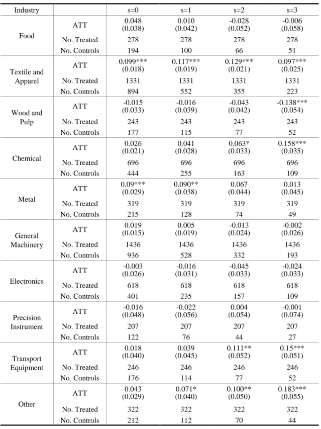
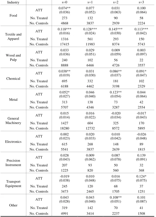
As a preliminary step, we first examine whether there are cross-industry differences in productivity gains from becoming exporters. To do so, we divided our sample into 10 sub-industries16

Nevertheless, Table 5 seems to show that there are some industry characteristics and repeated the matching procedure for each industry. Table 5 shows that productivity gains from learning-by-exporting are visible in the textile and apparel, chemical, metal, and transport equipment industries. However, we cannot find significant productivity gains in the food, wood and pulp, general machinery, precision instrument, and electronics industries. Roughly speaking, the former group of industries largely coincides with the area for which Korea is believed to have a comparative advantage. Therefore, the result can be interpreted as providing a piece of evidence supporting the hypothesis that involvement in exporting activities results in productivity gains. However, it is somewhat surprising that we can find no significant evidence for the existence of a learning-by-exporting effect in the electronics industry. Although we could conjecture that this reflects that many Korean producers in the electronics industry are the “frontier” producers, a more definitive assessment cannot be made until a more in-depth analysis is carried out.

16

They are food, textile and apparel, wood and pulp, chemical, metal, general machinery, electronics, precision instrument, transport equipment, and others.

24

that affect the strengths of the learning-by-exporting effect.

Table 5. Average Productivity Gain of Starters by Industry: BI Procedure

Industry s=0 s=1 s=2 s=3 Food ATT _(0.038) 0.048 _(0.042) 0.010 _(0.052) -0.028 _(0.058) -0.006 No. Treated 278 278 278 278 No. Controls 194 100 66 51 Textile and Apparel ATT 0.099*** (0.018) 0.117*** (0.019) 0.129*** (0.021) 0.097*** (0.025) No. Treated 1331 1331 1331 1331 No. Controls 894 552 355 223 Wood and Pulp ATT _(0.033) -0.015 _(0.039) -0.016 _(0.042) -0.043 -0.138*** _(0.054) No. Treated 243 243 243 243 No. Controls 177 115 77 52 Chemical ATT _(0.021) 0.026 _(0.028) 0.041 _(0.033) 0.063* 0.158*** _(0.035) No. Treated 696 696 696 696 No. Controls 444 255 163 109 Metal ATT 0.09*** _(0.029) 0.090** _{(0.038) (0.044)} 0.067 _(0.045) 0.013 No. Treated 319 319 319 319 No. Controls 215 128 74 49 General Machinery ATT _(0.015) 0.019 _(0.019) 0.005 _(0.024) -0.013 _(0.026) -0.002 No. Treated 1436 1436 1436 1436 No. Controls 936 528 332 193 Electronics ATT _(0.026) -0.003 _(0.031) -0.016 _(0.033) -0.045 _(0.033) -0.024 No. Treated 618 618 618 618 No. Controls 401 235 157 109 Precision Instrument ATT _(0.048) -0.016 _(0.056) -0.022 _(0.054) 0.004 _(0.074) -0.001 No. Treated 207 207 207 207 No. Controls 122 76 44 27 Transport Equipment ATT _(0.040) 0.018 _(0.045) 0.039 0.111** _(0.052) 0.15*** _(0.051) No. Treated 246 246 246 246 No. Controls 176 114 77 52 Other ATT _(0.029) 0.043 _(0.040) 0.071* 0.100** _(0.050) 0.183*** _(0.055) No. Treated 322 322 322 322 No. Controls 212 112 70 44

25

We next turn to the export destinations of industries as one possible factor explaining differential strengths of the learning-by-exporting effect estimated at the sub-group level of industries. As explained above and also in Loecker (2007), this hypothesis is based on the presumption that a learning-by-exporting effect will be stronger for plants that start exporting to more advanced countries, where the opportunities for learning new knowledge and technology are relatively abundant. Although Loecker (2007) examined this issue using plant-level information on the destination of exports, we do not have such information available for Korea. Instead, we examine whether plants in industries with a higher share of exports to advanced countries exhibit higher productivity gains.17

To do so, we first matched the direction of exports dataset at SITC 5 digit level complied from UNComtrade (Rev. 3) with the Mining and Manufacturing Survey dataset at KSIC

18

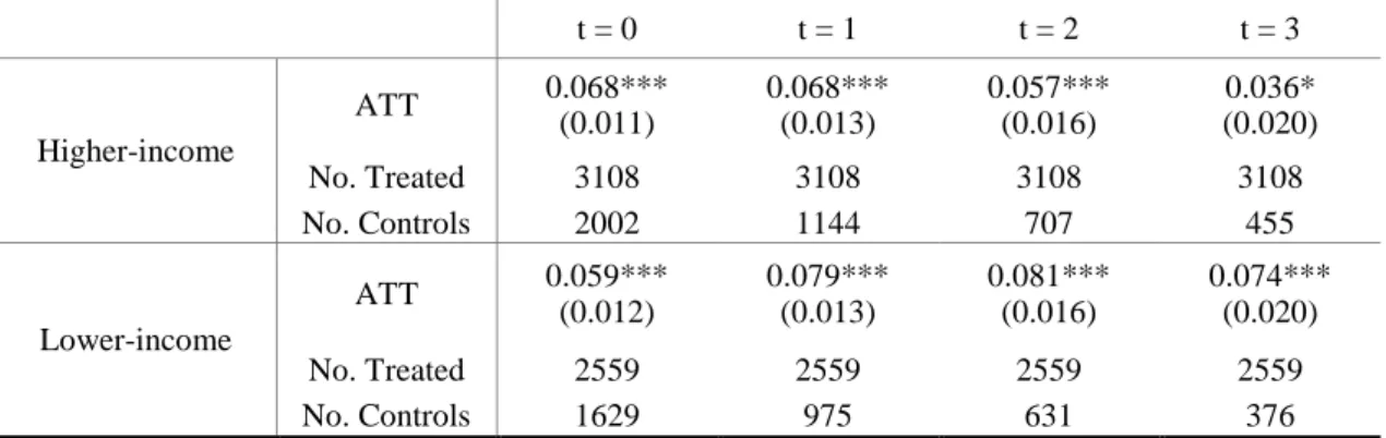
The estimated productivity gain for starters is reported in Table 6 for each three-digit level. Then, we classified Korea’s export destination countries into two groups: “lower-income” and “higher-income” countries. Here, higher-income countries are those with an average per capita GDP for the period from 1990 to 1998 larger than that of Korea. The remaining countries are lower-income countries. Next, for each of the 58 three-digit manufacturing industries, we calculated their shares of exports to lower-income and higher-income countries averaged over the same period. Then, we classified each industry into “higher-income” or “lower-income” group if its share of exports to higher-income countries is greater or smaller than lower-income countries, respectively.

17

In some respect, direction of exports is more likely to be an industry characteristic rather than plant characteristic.

18

26

group. At first glance, the results are not supportive of the hypothesis that the learning-by-exporting effect is more pronounced in industries with more of their exports directed to more advanced countries. In fact, the result is the other way around: Learning-by-exporting effect in the lower-income group is stronger than that of the higher-income group, although both are highly significant. We conjecture that the result is driven by the fact that the gain from participating in export markets depends on many factors conveniently branded as the benefits of openness. We believe that those factors must be interlinked in a very complicated fashion and a simple approach like ours cannot give the definite answer to this important question.

Table 6. Average Productivity Gain of Starters by Export Destinations: BI procedure t = 0 t = 1 t = 2 t = 3 Higher-income ATT 0.068*** (0.011) 0.068*** (0.013) 0.057*** (0.016) 0.036* (0.020) No. Treated 3108 3108 3108 3108 No. Controls 2002 1144 707 455 Lower-income ATT 0.059*** (0.012) 0.079*** (0.013) 0.081*** (0.016) 0.074*** (0.020) No. Treated 2559 2559 2559 2559 No. Controls 1629 975 631 376

Given the inadequate control of various factors that might be relevant for determining the degree of learning-by-exporting effect, the above results should not be taken as a definitive piece of evidence against the hypothesis that the learning-by-exporting effect is larger in industries with more of their exports directed to higher-income countries. We think that various industry as well as plant characteristics might also play a role here. Further analysis seems to be warranted to shed light on this issue.

27

5. Conclusion

This paper examined the presence of a learning-by-exporting effect utilizing a unique plant level panel data covering all manufacturing sectors in Korea. Korean experiences offer a good window of opportunity to analyze this issue in the sense that Korea is one of the best known success stories having achieved fast economic growth driven by “outward-oriented” development strategies.

We find clear and robust evidences for a learning-by-export effect. The total factor productivity gap between exporters and their domestic counterparts is significant and shows the tendency to widen during three years after entry into the export market. We also find that the beneficial effect of productivity gain is more pronounced for plants with a higher skill-intensity or higher share of exports in production.

Although this paper examined the learning-by-exporting effect, it should be born in mind that learning-by-exporting is just one of many channels through which the benefits of openness are realized. That is, the results of this paper does not at all exclude the possibility that the beneficial effects of openness are realized through various other channels, such as increases in consumer surpluses and improvements of allocation efficiency, knowledge spillovers and market-disciplining effects from imports, and improvement of scale efficiency, among others.

One interesting policy implication which arises from this paper might be that neoclassical orthodoxy of prescribing unconditional openness policy19

19

See Sachs and Warner (1995), for example.

might not be entirely warranted. If domestic absorptive capacity is complementary to the openness policy, as suggested by the evidence of larger a learning-by-exporting effect in

skill-28

intensive plants, then upgrading the quality of human capital might be necessary to more fully utilize the benefits from openness.

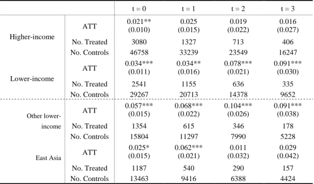
29

Tab le A.1. Average Productivity Gain of Starters by Firm Characteristics: LS Procedure Plant Characteristics s=0 s=1 s=2 s=3 Export Ratio Low ATT 0.036*** (0.011) 0.001 (0.016) 0.021 (0.022) -0.005 (0.026) No. Treated 2129 972 526 304 No. Controls 76576 54362 38237 27244 Medium ATT 0.019 (0.012) 0.071*** (0.018) 0.052** (0.024) 0.054 (0.033) No. Treated 1835 769 424 222 No. Controls 76576 54362 38237 27244 High ATT 0.054*** (0.013) 0.109*** (0.019) 0.105*** (0.025) 0.074** (0.035) No. Treated 1686 747 402 216 No. Controls 76576 54362 38237 27244 Skill Intensity Low ATT -0.014 (0.016) 0.004 (0.026) 0.086** (0.037) 0.099** (0.050) No. Treated 1086 406 191 90 No. Controls 30592 20469 13645 8953 Medium ATT 0.026*** (0.009) 0.046*** (0.013) 0.043*** (0.017) 0.025 (0.025) No. Treated 3306 1517 844 472 No. Controls 37772 27997 20343 14916 High ATT 0.062*** (0.017) 0.057** (0.025) 0.063** (0.033) 0.104*** (0.041) No. Treated 1258 569 319 181 No. Controls 8212 5896 4249 3120 Number Of Workers Low ATT 0.056*** (0.015) 0.074*** (0.026) 0.108*** (0.042) 0.082 (0.060) No. Treated 1443 423 153 68 No. Controls 39564 25645 16386 10862 Medium ATT 0.057*** (0.010) 0.059*** (0.014) 0.069*** (0.018) 0.084*** (0.024) No. Treated 3161 1407 764 411 No. Controls 33433 25722 19349 14321 High ATT 0.031 (0.019) -0.023 (0.024) -0.036 (0.030) 0.035 (0.040) No. Treated 1046 662 437 264 No. Controls 3579 2995 2502 2061 R&D None ATT 0.033*** (0.008) 0.041*** (0.012) 0.055*** (0.015) 0.039* (0.022) No. Treated 4678 2040 1080 598 No. Controls 73923 52426 36829 26816 Low ATT 0.005 (0.035) -0.008 (0.041) 0.000 (0.049) 0.066 (0.066) No. Treated 351 188 122 66 No. Controls 825 605 455 302 Medium ATT -0.007 (0.030) 0.031 (0.038) -0.024 (0.056) 0.055 (0.068) No. Treated 446 199 114 61 No. Controls 1201 881 637 453 High ATT 0.049 (0.047) -0.014 (0.062) -0.029 (0.086) 0.089 (0.132) No. Treated 175 65 38 18 No. Controls 627 424 298 180

30

Table A.2. Productivity Gain of Starters by Industry: LS Procedure

Industry s=0 s=1 s=2 s=3 Food ATT 0.074** (0.036) 0.077 (0.052) 0.031 (0.063) 0.100 (0.064) No. Treated 273 132 90 58 No. Controls 4868 3837 2939 2224 Textile and Apparel ATT 0.118*** (0.016) 0.128*** (0.024) 0.145*** (0.030) 0.113*** (0.042) No. Treated 1316 561 293 150 No. Controls 17415 11983 8374 5743 Wood and Pulp ATT 0.033 (0.036) 0.029 (0.051) 0.009 (0.059) 0.003 (0.097) No. Treated 240 102 56 22 No. Controls 8888 6466 4726 3557 Chemical ATT 0.038** (0.019) 0.031 (0.030) 0.086** (0.037) 0.091* (0.047) No. Treated 695 332 181 102 No. Controls 6188 4462 3198 2329 Metal ATT 0.052* (0.027) 0.046 (0.040) 0.123** (0.054) 0.044 (0.064) No. Treated 313 138 73 42 No. Controls 5707 4346 3287 2554 General Machinery ATT 0.015 (0.014) 0.016 (0.022) -0.020 (0.034) -0.017 (0.043) No. Treated 1427 604 325 170 No. Controls 18280 12732 8572 5895 Electronics ATT 0.002 (0.023) 0.020 (0.033) 0.010 (0.042) -0.026 (0.048) No. Treated 615 268 148 89 No. Controls 5541 3837 2639 1815 Precision Instrument ATT 0.028 (0.043) 0.009 (0.062) 0.087 (0.078) 0.139 (0.091) No. Treated 207 93 50 32 No. Controls 1225 820 560 368 Transport Equipment ATT -0.019 (0.038) 0.010 (0.048) 0.016 (0.075) 0.124* (0.075) No. Treated 245 120 68 37 No. Controls 3473 2465 1705 1251 Other ATT 0.043 (0.028) 0.043 (0.040) 0.108** (0.051) 0.101 (0.087) No. Treated 319 142 70 41 No. Controls 4991 3414 2237 1508

31

Table A.3. Average Productivity Gain of Starters by Export Destinations: LS Procedure t = 0 t = 1 t = 2 t = 3 Higher-income ATT 0.021** _{(0.010) (0.015)} 0.025 _(0.022) 0.019 _(0.027) 0.016 No. Treated 3080 1327 713 406 No. Controls 46758 33239 23549 16247 Lower-income ATT 0.034*** _(0.011) 0.034** _(0.016) 0.078*** _(0.021) 0.091*** _(0.030) No. Treated 2541 1155 636 335 No. Controls 29267 20713 14378 9652 Other lower-income ATT 0.057*** _(0.015) 0.068*** _(0.022) 0.104*** _(0.026) 0.091*** _(0.038) No. Treated 1354 615 346 178 No. Controls 15804 11297 7990 5228

East Asia ATT

0.025* (0.015) 0.062*** (0.021) 0.011 (0.032) 0.029 (0.042) No. Treated 1187 540 290 157 No. Controls 13463 9416 6388 4424

32

References

Albonorez, F. and Marco Ercolani (2007), “Learning by Exporting: Do Firm Characteristics Matter? Evidence from Argentinian Panel Data,” Working Paper, University of Birmingham.

Aw, B. Y. and G. Batra (1998), “Technology, Exports, and Firm Efficiency in Taiwanese Manufacturing,” Economics of Innovation and New Technology, 7(1): 93-113.

Aw, B. Y. and A. Hwang, (1995), “Productivity and the Export Market: A Firm-Level Analysis,” Journal of Development Economics, 47(2): 313-32.

Aw, B.Y., S. Chung and M. J. Roberts (2000), “Productivity and Turnover in the Export Market: Micro-level Evidence from the Republic of Korea and Taiwan(China),” The World Bank Economic Review, 14(1): 65-90.

Aw, B. Y., X. Chen, and M. J. Roberts (2001), “Firm-level Evidence on Productivity

Differentials, Turnover and Exports in Taiwanese Manufacturing,” Journal of

Development Economics, 66(1): 51-86.

Bartel, A.P. and Lichtenberg, F.R. (1987), “The Comparative Advantage of Educated Workers in Implementing New Technology, ” Review of Economics and Statistics, 69(1): 1-11.

Benhabib, J. and M. Spiegel (1994), “The Role of Human Capital in Economic

Development: Evidence from Aggregate Cross-country Data,” Journal of

Monetary Economics, 34, 143-73.

Benhabib, J. and M. Spiegel (2005), “Human Capital and Technology Diffusion,” in

Aghion, Philippe and Steven N. Durlaf eds. Handbook of Economic Growth,

Elsevier, North-Holland.

Becker, S. O., and Andrea Ichino (2002), “Estimation of Average Treatment Effects Based on Propensity Scores,” The Stata Journal, 2: 358-77.

Bernard, A. B. and J. B. Jensen (1999a), “Exceptional Exporter Performance: Cause, Effect, or Both?”, Journal of International Economics, 47, 1-25.

Bernard, A. B. and J. B. Jensen (1999b), “Exporting and Productivity,” NBER Working Paper, No.7135.

Bernard, A. B. and J. Wagner (1997), “Exports and Success in German Manufacturing,” Weltwirtschaftliches Archive, 133(1): 134-57.

33

Clerides, S. K., S. Lach and J. R. Tybout (1998), “Is Learning by Exporting Important?

Micro-Dynamic Evidence from Colombia, Mexico, and Morocco,” The Quarterly

Journal of Economics, 113: 903-47.

Foster, A. D. and Rosenzweig, M. R. (1995), “Learning by Doing and Learning from Others: Human Capital and Technical Change in Agriculture” Journal of Political Economy, 103(6): 1176-209.

Girma, S., Greenaway, D., and R. Kneller (2002), “Does Exporting Lead to Better

Performance? A Micro econometric Analysis of Matched Firms,” GEP Research

Paper, No.02/09.

Good, David H. (1985), “The Effect of Deregulation on the Productive Efficiency and Cost Structure of the Airline Industry, Ph.D. dissertation, University of Pennsylvania.

Good, David H., M. Ishaq Nadiri, and Robin Sickles (1999), “Index Number and

Factor Demand Approaches to the Estimation of Productivity,” In Handbook of

Applied Econometrics: Micro Econometrics, eds. H. Pesaran and Peter Schmidt, Blackwell Publishers, Oxford, UK.

Hahn, Chin Hee. (2004), “Exporting and Performance of Plants: Evidence from

Korean Manufacturing,” NBER Working Paper, No.10208.

Heckman, J., Ichimura, H., and P. Todd (1997), “Matching as an Econometric Evaluation Estimator,” Review of Economic Studies, 65: 261-94.

Kimura, F., Hayakawa, K. and T. Matsuura. (2009), “Gains from Fragmentation at the

Firm Level: Evidence from Japanese Multinationals in East Asia,” ERIA

Discussion Paper, No.2009-07.

Krueger, A. (1997), “Trade Policy and Economic Development: How We Learn,” American Economic Review, 87(1): 1-22.

Loecker, J. K. D., (2007), “Do Exports Generate Higher Productivity? Evidence from Slovenia,” Journal of International Economics, 73(1): 69-98.

Leuven, E., and B. Sianesi (2003), “PSMATCH2: Stata Module to Perform Full Mahalanobis and Propensity Score Matching, Common Support Graphing, and Covariate Imbalance Testing,” Statistical Software Components S432001, Boston University

34

Observational Studies for Causal Effects,” Biometrica, 70(1): 41-55.

Sachs, Jeffrey, and A. Warner (1995), “Economic Reform and the Process of Global Integration,” Brookings Papers on Economic Activity, 1: 1-95.

Tybout, J. R., (2000), “Manufacturing Firms in Developing Countries: How Well Do They Do, and Why?,” Journal of Economic Literature, 38, 11-44.

Welch, F. (1975), “Human Capital Theory: Education, Discrimination, and Life Cycles,” American Economic Review, 65(2): 63-73.

ERIA Discussion Paper Series

No. Author(s) Title Year

2009-09 Mitsuyo ANDO and

Akie IRIYAMA

International Production Networks and Export/Import Responsiveness to Exchange Rates:

The Case of Japanese Manufacturing Firms

Mar 2009

2009-08 Archanun

KOHPAIBOON

Vertical and Horizontal FDI Technology Spillovers: Evidence from Thai Manufacturing

Mar 2009

2009-07

Kazunobu HAYAKAWA, Fukunari KIMURA, and Toshiyuki MATSUURA

Gains from Fragmentation at the Firm Level: Evidence from Japanese Multinationals in East Asia

Mar 2009

2009-06 Dionisius A. NARJOKO

Plant Entry in a More Liberalised Industrialisation Process: An Experience of Indonesian

Manufacturing during the 1990s

Mar 2009

2009-05

Kazunobu HAYAKAWA, Fukunari KIMURA, and Tomohiro MACHIKITA

Firm-level Analysis of Globalization: A Survey Mar

2009

2009-04 Chin Hee HAHN and

Chang-Gyun PARK

Learning-by-exporting in Korean Manufacturing: A Plant-level Analysis

Mar 2009

2009-03 Ayako OBASHI Stability of Production Networks in East Asia:

Duration and Survival of Trade

Mar 2009

2009-02 Fukunari KIMURA

The Spatial Structure of Production/Distribution Networks and Its Implication for Technology Transfers and Spillovers

Mar 2009

2009-01 Fukunari KIMURA and

Ayako OBASHI

International Production Networks: Comparison between China and ASEAN

Jan 2009

2008-03 Kazunobu HAYAKAWA

and Fukunari KIMURA

The Effect of Exchange Rate Volatility on International Trade in East Asia

Dec 2008

2008-02

Satoru KUMAGAI, Toshitaka GOKAN, Ikumo ISONO, and Souknilanh KEOLA

Predicting Long-Term Effects of Infrastructure Development Projects in Continental South East Asia: IDE Geographical Simulation Model

Dec 2008

2008-01

Kazunobu HAYAKAWA, Fukunari KIMURA, and Tomohiro MACHIKITA

Firm-level Analysis of Globalization: A Survey Dec