Learning Generative Models for Multi-Activity Body Pose Estimation

DOI 10.1007/s11263-008-0158-0

Learning Generative Models for Multi-Activity Body Pose

Estimation

Tobias Jaeggli·Esther Koller-Meier·Luc Van Gool

Received: 30 January 2008 / Accepted: 11 July 2008 / Published online: 31 July 2008 © Springer Science+Business Media, LLC 2008

Abstract We present a method to simultaneously estimate 3D body pose and action categories from monocular video sequences. Our approach learns a generative model of the relationship of body pose and image appearance using a sparse kernel regressor. Body poses are modelled on a low-dimensional manifold obtained by Locally Linear Em-bedding dimensionality reduction. In addition, we learn a prior model of likely body poses and a dynamical model in this pose manifold. Sparse kernel regressors capture the nonlinearities of this mapping efficiently. Within a Recur-sive Bayesian Sampling framework, the potentially multi-modal posterior probability distributions can then be in-ferred. An activity-switching mechanism based on learned transfer functions allows for inference of the performed ac-tivity class, along with the estimation of body pose and 2D image location of the subject. Using a rough foreground segmentation, we compare Binary PCA and distance trans-forms to encode the appearance. As a postprocessing step, the globally optimal trajectory through the entire sequence is estimated, yielding a single pose estimate per frame that is consistent throughout the sequence. We evaluate the algo-rithm on challenging sequences with subjects that are alter-nating between running and walking movements. Our ex-periments show how the dynamical model helps to track

T. Jaeggli (

e-mail:[email protected] E. Koller-Meier e-mail:[email protected] L. Van Gool e-mail:[email protected] L. Van Gool

KU Leuven, Leuven, Belgium

through poorly segmented low-resolution image sequences where tracking otherwise fails, while at the same time reli-ably classifying the activity type.

Keywords Monocular pose estimation·Machine

learning·Dimensionality reduction·Activity recognition· Human locomotion

1 Introduction

Monocular body pose estimation is difficult, because a cer-tain input image can often be interpreted in different ways. Image features computed from the silhouette of the tracked figure hold rich information about the body pose, but sil-houettes are inherently ambiguous, e.g. due to the Necker reversal. Through the use of prior models this problem can be alleviated to a certain degree, but in many cases the in-terpretation is ambiguous and multi-valued throughout the sequence.

Several approaches have been proposed to tackle this problem, they can be divided into discriminative and gen-erative methods. Discriminative approaches directly infer body poses given an appearance descriptor, whereas genera-tive approaches provide a mechanism to predict the appear-ance features given a pose hypothesis, which is then used in a generative inference framework such as particle filtering or numerical optimisation.

Recently, statistical methods have been introduced that can learn the relationship of pose and appearance from a training data set. They often follow a discriminative ap-proach and have to deal explicitly with the nonfunctional nature of the multi-valued mapping from appearance to pose (Rosales and Sclaroff2001; Thayananthan et al.2006;

Sminchisescu et al.2005; Agarwal and Triggs2005; Jaeg-gli et al. 2006). Generative approaches on the other hand typically use hand crafted geometric body models to predict image appearances (e.g. Sidenbladh et al.2000, see Forsyth et al.2006; Moeslund et al.2006for an overview).

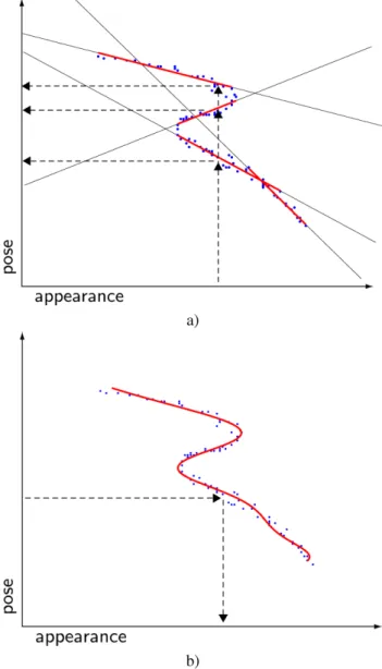
We propose to combine the generative methodology with a learning based statistical approach. The mapping from pose to appearance is single-valued and can thus be seen as a nonlinear regression problem. We approximate the map-ping with a Relevance Vector Machine (RVM) kernel re-gressor (Tipping 2000) that is efficient due to its sparsity. See Fig.1for an illustration of the one-to-many regression problem. Although single-valued, the appearance prediction will be subject to uncertainty, because other factors than just the body configuration (pose) may affect appearance (cloth-ing, physical constitution, lighting conditions etc.). This is taken into account by learning the prediction variances of the mapping.

The observations are available in the form of roughly seg-mented monocular image sequences that are obtained by a pre-processing step such as motion segmentation, back-ground subtraction or other. A main focus of the pro-posed approach lies on the ambiguities and uncertainties that are inherent in body tracking from such input. Recursive Bayesian Sampling (Isard and Blake1998a; Doucet et al.

2000a) offers a framework for dealing with non-Gaussian and multimodal body pose posteriors and allows us to in-tegrate the nonlinear learned dynamical model. However, sampling-based algorithms are generally not applicable for inference in high-dimensional state spaces like the space of body poses. We therefore use Locally Linear Embedding (LLE, Roweis and Saul2000) to find a low-dimensional em-bedding of our 60-dimensional pose parametrisation. With 4 LLE dimensions, the considered motions can be captured reasonably well.

The tasks of body pose estimation and activity recogni-tion are strongly related. While a sequence of inferred body poses might be used for activity recognition, a known ac-tivity class can also help the pose estimation, e.g. by se-lecting an appropriate context specific prior. The proposed method estimates 3D body pose and action categories simul-taneously. We learn strong dimensionality-reduced models of feasible body poses that belong to a certain activity or motion pattern, as well as the temporal evolution of the body poses over time. Furthermore, the transition functions be-tween different activities are learned from training data too. In this article we investigate typical human motion patterns such as walking and running. Rather than learning a unified representation that contains both walking and running mo-tions, we learn separate activity specific models that allow us to explicitly recognise the performed activity along with the pose estimation, using a switching mechanism of the in-ference algorithm.

Fig. 1 Illustration of a discriminative one-to-many mapping with a mixture of linear regressors (a), and of a generative mapping from pose space to appearance space with a single nonlinear regressor (b)

The main contributions of this article are the generative appearance modelling, the tracking in a LLE-reduced pose representation with a nonlinear dynamical model, simulta-neous recognition of multiple action categories, and the ex-traction of a globally optimal trajectory through the entire sequence.

2 Related Work

There is a wide variety of literature about body pose estima-tion and tracking (see Forsyth et al.2006for an overview). Here we will have a look at the application of statisti-cal methods that infer poses from one or multiple camera streams. Many authors adopt a discriminative strategy to

infer poses directly from image descriptors (Rosales and Sclaroff2001; Thayananthan et al.2006; Sminchisescu et al.

2005; Agarwal and Triggs 2004a, 2005; Grauman et al.

2003; Sun et al.2006).

Synchronous image sequences from multiple cameras typically provide enough information to resolve ambigui-ties. The discriminative mapping from descriptors to body poses can thus be modelled using a single regressor. In Sun et al. (2006), a new image descriptor is introduced based on a voxel representation that is derived from segmented images of multiple cameras. This descriptor can then be directly mapped into pose space. In Grauman et al. (2003) multi-ple silhouette image descriptors and corresponding pose de-scriptors are concatenated and modelled with a mixture of Probabilistic PCA; poses can then be inferred given multi-ple views of the subject.

Monocular approaches have to deal with the one-to-many discriminative mapping from appearance to pose. This is-sue is explicitly addressed in Rosales and Sclaroff (2001), Thayananthan et al. (2006), Sminchisescu et al. (2005), Agarwal and Triggs (2005), Jaeggli et al. (2006) by learn-ing multiple mapplearn-ings in parallel as a mixture of regres-sors. In order to choose between the different hypotheses that the different regressors deliver, Rosales and Sclaroff (2001), Thayananthan et al. (2006) use a geometric model that is projected into the image to verify the hypotheses. In-ference is performed for each frame independently in Ros-ales and Sclaroff (2001). In Thayananthan et al. (2006) a temporal model is included using a bank of Kalman filters, and a Viterbi algorithm finds a path through the peaks of the posterior distribution. In Sminchisescu et al. (2005), Agar-wal and Triggs (2005), Jaeggli et al. (2006) gating functions are learned along with the regressors in order to pick the right regressor(s) for a given appearance descriptor. The dis-tribution is propagated analytically in Sminchisescu et al. (2005), and temporal aspects are included in the learned dis-criminative mapping, whereas Agarwal and Triggs (2005) adopts a generative sampling-based tracking algorithm with a first-order autoregressive dynamic model. In Jaeggli et al. (2006) discriminative analytical inference and generative sample-based inference are combined in a Rao-Black well-ised particle filter. This allows for efficient inference in the high dimensional pose space in combination with the non-parametric posterior distributions that occur when the 2D image location has to be inferred by the algorithm as well.

The mentioned purely discriminative approaches work in a bottom-up fashion, starting with the computation of the image descriptor, which requires the location of the figure in the images to be known beforehand. When including 2D bounding box estimation in the tracking problem, a learned dynamical model of the appearance might help the bounding box tracking, and avoid losing the subject when it is tem-porarily occluded. To this end, Lim et al. (2006) learns a

subject-specific dynamic appearance model from a small set of initial frames, consisting of a low-dimensional embed-ding of the appearances and a motion model. This model is used to predict the location and appearance of the fig-ure in futfig-ure frames, within a CONDENSATION tracking framework. Similarly, low-dimensional embeddings of ap-pearance (silhouette) manifolds are found using LLE in El-gammal and Lee (2004), where additionally the mapping from the appearance manifold to 3D pose in body joint space is learned using radial basis function (RBF) inter-polants, allowing for pose inference from sequences of sil-houettes.

Instead of modelling manifolds in appearance space, Wang et al. (2006), Sminchisescu and Jepson (2004), Li et al. (2006) work with low dimensional embeddings of body poses. In Wang et al. (2006), Urtasun et al. (2006), the low-dimensional pose representation, its dynamics, and the mapping back to the original pose space are learned in a unified framework. This approach does not include a learned statistical model of image appearance. Our method also models pose manifolds rather than appearance mani-folds, because the pose manifold has fewer self-in tersec-tions than the appearance manifold, making the dynamics and tracking less ambiguous.

To model the nonlinear dynamics of human motion, dif-ferent approaches have been proposed. In Pavlovic et al. (2001), Agarwal and Triggs (2004b), Li et al. (2007) mix-tures of linear autoregressive motion models (respectively piecewise linear models) were used, where the inference al-gorithm switches between a number of discrete states cor-responding to the different linear models. These models are learned using EM-like optimisation. Our method is in line with Wang et al. (2006), Urtasun et al. (2006), Lee and El-gammal (2007), where temporal predictions are obtained us-ing nonlinear regression. In such a way, smooth motion flow fields over the entire pose space can be learned directly. In contrast to a piecewise linear model, there is thus no need to learn a finite number of states that have no semantic meaning that is of interest for our task, and in particular we don’t have to select the optimal number of mixture compo-nents.

Most related to our approach are two recent publications that also model the appearance of moving persons in a gen-erative way. In Lee and Elgammal (2007) a low dimensional embedding of the kinematics is obtained using joint an-gles data. View-based nonlinear mapping functions from the kinematic manifolds to multi-view appearance are used to infer poses in a Bayesian tracking framework. They model the view dependencies of the appearance on a low-dimen-sional posture-independent view manifold. In Navaratnam et al. (2007) a shared low-di mensional latent space with nonlinear mappings into the pose and appearance spaces is learned using an extension of the GP-LVM (Lawrence2005)

framework. The graphical structure of the learned model is thus similar to the method proposed in this article, with the exception of the dynamics, which are not explicitly mod-elled in Navaratnam et al. (2007). Furthermore the authors propose the use of unlabelled data to improve the learned model.

Regarding activity switching, Isard and Blake (1998b) have proposed a state switching mechanism, where differ-ent dynamical models are chosen, depending on a discrete state variable. In our approach, the different states (activ-ities) involve separate models for pose, dynamics and ap-pearance.

Our approach differs from the above-mentioned papers in that it simultaneously tracks in a state space that includes body pose, 2D bounding box location and a discrete activity label. Furthermore, we present a full-fledged pipeline with generative rather than discriminative modelling of the ap-pearance, entirely based on learned models. The framework is built-up in a module based manner. Some choices of pre-cise statistical methods that are applied for the individual modules are mainly based on practical considerations (e.g. efficiency, sparsity). They could be substituted by equiva-lent methods, like e.g. Isomap (Tenenbaum et al.2000) in-stead of LLE, and regularised kernel regressors or Gaussian processes instead of RVMs.

The remainder of this paper is organised as follows. Sec-tion3introduces our learned models. In Sect.4the sample-based inference algorithm is presented and Sect. 5 shows experimental results on different video sequences.

3 Statistical Modelling

Figure2a shows an overview of the tracking framework, re-duced to a single activity category for clarity. Central el-ement is the low-dimensional body pose parametrisation, with learned mappings back to the original pose space and into the appearance space. In this section all elements of the framework will be described in detail.

Our models were trained on motion capture data sets of different subjects, running and walking at different speeds. Walking and running training examples were separately processed to train activity specific models.

3.1 Pose and Motion Model

Representations for the full body pose configuration are high dimensional by nature; our current representation is based on 3D joint locations of 20 body locations such as hips, knees and ankles (see Fig.2b, but any other representation (e.g. based on relative orientations between neighbouring limbs) can easily be plugged into the framework. To allevi-ate the difficulties of high dimensionality in both the learn-ing and inference stages, a dimensionality reduction step identifies a low dimensional embedding of the body pose representations. We use Locally Linear Embedding (LLE) (Roweis and Saul 2000), which approximately maintains the local neighbourhood relationships of each data point and allows for global deformations (e.g. unrolling) of the dataset/manifold.

LLE dimensionality reduction is performed on all poses in the data set that belong to a certain activity, and expresses

Fig. 2 (a) An overview of the tracking framework. Solid

arrows represent signal flow

during inference, the dashed

arrow stands for the nonlinear

dimensionality reduction during training. The figure refers to equations in Sect.3. (b) Body pose representation as a number of 3D joint locations.

(c) Distance transformed image descriptordt (Y ). Each pixel value is proportional to the distance to the silhouette, and its sign indicates whether the pixel lies inside the silhouette

Fig. 3 (Color online) Low-dimensional manifold of walking data obtained by Locally Linear Embedding. Three dimensions of the four-dimensional representation are visualised here, from two differ-ent views. The differdiffer-ent colours indicate differdiffer-ent walking speeds (red: 2.5 km/h, green: 4.2 km/h, blue: 6 km/h)

each data point in a space of desired low dimensionality (see also Fig.3). However, LLE does not provide explicit map-pings between the two spaces, that would allow to project new data points (that were not contained in the original data set) between them. Therefore, we model the reconstruction projection from the low-dimensional LLE space to the orig-inal pose space with a kernel regressor.

X=fp(x)=Wpp(x) (1)

Here, X andx are the body pose representations in orig-inal resp. LLE-reduced spaces, p is a vector of kernel

functions, andWp is a sparse matrix of weights, which are

learned with a Relevance Vector Machine. We use Gaussian kernel functions, computed at the training data locations. Separate models are learned for the two distinct activities,

f_pw(xw)and f_pr(xr). In the following we will use super-scripts (e.g.wfor walk andr forrun) to indicate activity categories in the notation if necessary and omit them if the same formulation holds for all actions.

The training examples form a periodic twisted ‘ring’ in LLE space, with a curvature that varies with the phase within the periodic movement. A linear dynamical model, as often used in tracking applications, is not suitable to predict fu-ture poses on this curved manifold. We view the nonlinear

dynamics as a regression problem, and model it using an-other RVM regressor, yielding the following dynamic prior,

pd(xt|xt−1)=N(xt;xt−1+fd(xt−1)T, d), (2)

where fd(xt−1)=Wdd(xt−1) is the nonlinear mapping from poses to local velocities in LLE pose space,T is the

time interval between the subsequent discrete timestepst−1 andt, anddis the variance of the prediction errors of the

mapping, computed on a hold-out data set that was not used for the estimation of the mapping itself. Again, the dynamics are learned separately for the different action categories.

Not all body poses that can be expressed using the LLE pose parametrisation do correspond to valid body configu-rations that can be reached with a human body. The motion model described so far does only include information about the temporal evolution of the pose, but no information about how likely a certain body pose is to occur in general. In other words, it does not yet provide any means to restrict our tracking to feasible body poses. The additional prior knowl-edge about feasible body poses, or likely poses for a given activity, is introduced as a static prior that is modelled with a Gaussian Mixture Model (GMM),

ps(x)= C

c

pcN(x;μc, c), (3)

withC the number of mixture components andpc,μcand

c the mixture proportions and parameters of the Gaussian

components. The influence of this pose prior can be kept low, avoiding a distortion of the tracking results towards typ-ical average motion. We introduce a weighting factorλ >1 and obtain the following formulation for the temporal prior by combination with the dynamic priorpd(xt|xt−1). p(xt|xt−1)∝pd(xt|xt−1) ps(xt)

1

λ (4)

We also want to model the transition between the considered action categories, that each have their own low dimensional pose parametrisation expressed in distinct LLE spaces. In-formally, we want to find walking poses that are very similar to a given running pose and vice versa, since we know that the transition is performed smoothly, without any sudden or jerky ‘jump’ of the body configuration.

Given our distinct training sets of walking and running poses, two sets of training pairs are generated by looking for the most similar running pose for every walking pose and vice versa, and the nonlinear mapping between these pairs is modelled using two sparse kernel regressors f_switchr→w(xr)

andf_switchw→r(xw). This can be generalised to more action cat-egories1and leads to the following motion model, where the

1_{The number of transitions grows quadratically with the number of}

state space from (4) is augmented by a discrete state vari-ableat. p(xt, at|xt−1, at−1) ∝ pnoswitch pat(xt|xt−1) ifat=at−1 pswitch pat−1→at(xt|xt−1) else (5)

Here, the motion model for the case of activity switch-ingpat−1→at_(x

t|xt−1)is modelled as a normal distribution around the pose predicted by the regressor fat−1→at

switch . The

probabilities that an activity transition does or does not oc-cur are denotedpswitchandpnoswitch. In the case of more than two activity categories, these transition probabilities could be represented as a transition matrix with thepa_noswitchof the different categoriesaon the diagonal.

3.2 Appearance Model

The representation of the subject’s image appearance is based on a rough figure-ground segmentation. Under realis-tic imaging conditions, it is not possible to get a clean silhou-ette, therefore the image descriptor has to be robust to noisy segmentations to a certain degree. We consider two types of image descriptors, distance transformsdt (Y )(Bailey2004) of segmented figures with a subsequent linear PCA dimen-sionality reduction step (see Fig.2c), and a representation obtained by applying Binary PCA (BPCA) (Zivkovic and Verbeek2006) to binary foreground images. Both image de-scriptors are computed from the content of a bounding box around the centroid of the figure, and 10 to 20 PCA resp. BPCA components have been found to yield good recon-structions. We introduce the following notation for the com-putation of these descriptors and the projection on the re-spective subspaces given the raw pixel imageY:

yDT=V (dt (Y )−μ) yBPCA=BPCA(Y )

(6)

In this equation, μ andV are the mean and basis vectors obtained by PCA. BPCA(Y ) anddt (Y ) are nonlinear op-erations, in the BPCA case the projection on the subspace is done iteratively (see Zivkovic and Verbeek2006). As we will see later, it is useful in some situation to consider the inverse operation that projects the image descriptors yDT andyBPCAback into high dimensional pixel space and trans-forms it into binary images or foreground (f g) probability maps. From the descriptors we compute probability maps via the sigmoid function σ (.). In the case of the distance transformed descriptor this is based on the intuition that the foreground/background probabilities are higher far away from the silhouette, and lower very close to the silhouette.

BPCA reconstruction is also based on the sigmoid function (Zivkovic and Verbeek2006).

p(Y=f g|yDT)∝σ (VTyDT+μ) p(Y=f g|yBPCA)∝σ (VTyBPCA+μ)

(7)

Again,μandV are the mean and basis vectors from linear resp. binary PCA.

Now that we have seen how to compute image descrip-tors from segmented images and back, we will look how the image appearance is linked to the LLE body pose represen-tationx. We will model the generative mapping from posex

to image descriptorsy that allows to predict image appear-ance given pose hypotheses and fits well into generative in-ference algorithms such as recursive Bayesian sampling. In addition to the local body posex, the appearance depends on the global body orientationω(rotation around vertical axis).

p(y|x, ω)=N(y;fa(x, ω), a)

fa(x, ω)=Waa(x, ω)

(8)

Here, the functional mappingfa(x, ω)is approximated by

a sparse kernel regressor (RVM) with weight matrix Wa

and kernel functionsa(x).a is the prediction variance

matrix, it indicates which dimensions of the descriptor y

can be well predicted and which cannot, and thus accounts for the fact that the prediction ofy will always be subject to uncertainty. a is estimated from a hold-out set of the

original training data and restricted to a diagonal matrix for simplicity.

4 Inferring Image Position, Orientation, Activity and Pose

In this section we will show how the 2D image posi-tion, body orientaposi-tion, activity category, and body pose of the subject are simultaneously estimated given a video se-quence, by using the learned models from the previous sec-tion within the framework of recursive Bayesian sampling. Both pose estimation and image localisation can benefit from the coupling of pose and image location. For example, the known current pose and motion pattern can help to track through occlusions and distinguish subjects from each other. We therefore believe that tracking should happen jointly in the entire state space,

t= [at, ωt, ut, vt, wt, ht, xt], (9)

consisting of the discrete activitya, orientationω, the 2D bounding box parameters (position, width and height)u,v,

w,h, and the body posex.

Despite the reduced number of pose dimensions, we face an inference problem in 10-dimensional space. Having a

good sample proposal mechanism like our dynamical model is crucial for the Bayesian recursive sampling to run effi-ciently with a moderate number of samples. For the monoc-ular sequences we consider, the posteriors can be highly multimodal. For instance a typical walking sequence, e.g. observed from a side view, has two obvious posterior modes, shifted 180 degrees in phase, corresponding to the left resp. the right leg swinging forward. When taking the orientation of the figure into account, the situation gets even worse, and the modes are no longer well separated in state space, but can be close in both pose and orientation. Our experiments have shown that a strong dynamical model is necessary to avoid confusion between these posterior modes and reduce ambiguities. Some posterior multimodalities do however re-main, since they correspond to a small number of different interpretations of the images, which are all valid and feasible motion patterns.

The precise inference algorithm is very similar to classi-cal CONDENSATION (Isard and Blake 1998a), with nor-malisation of the weights and resampling at each time step. If we neglect the activity switching mechanism for a moment, the prior and likelihood for our inference prob-lem are obtained by extending (4) and (8) to the full state space. In our implementation, the dynamical prior

pd(it|it−1)serves as the sample proposal function. It con-sists of the learned dynamical pose prior from (2), and a simple motion model for the remaining state variables

θ= [ωt, ut, vt, wt, ht].

pd(it|it−1)=pd(xti|xti−1)N(θ

i

t;θti−1, θ) (10)

In practice, one may want to use a standard autoregres-sive model for propagating θ, omitted here for notational simplicity. We assume statistical independence between the body posex and the state variables θ in (10), since mod-elling these dependencies would imply restricted camera motions (e.g. static camera). The static prior over likely body poses (3) and the likelihood (8) are then used for as-signing weightswi to the samples.

w_ti∝p(y_ti|i_t)ps(it) 1 λ =_p(yi t|xti, ωit)ps(xit) 1 λ ₍₁₁₎

Here, i is the sample index, and yi_t is the image descrip-tor computed at timet from the sampled bounding box (ui_t,

vi_t, wi_t,hi_t). Note that our choice for sample proposal and weighting functions differs from CONDENSATION in that we only use one component (pd) of the prior (4) as a

pro-posal function, whereas the other component (ps) is

incor-porated in the weighting function.

4.1 Likelihood Computation in Image Space or on a PCA Subspace

Our framework has a generative flavour, since we model the pdf of the appearance given the body pose in a top-down

manner. The computation of the image descriptor and pro-jection on the subspace and back can be issued in both direc-tions, as seen in (6) and (7). One possibility is to compute the image descriptors in a bottom-up manner and project them onto the PCA or BPCA subspace (6), where the likelihood is then directly obtained using (8).

Alternatively, in a purely generative top-down manner, we can predict whether we expect a certain pixel to be fore-ground or backfore-ground given a pose hypothesis. This is done by concatenating the mapping fa(x, ω) from (8) and the

projection of the appearance descriptor into full appearance space (image space) (7). This yields a discrete 2D probabil-ity distribution of foreground probabilities Seg over the pix-els p in the bounding box. From this pdf, a likelihood mea-sure can then be derived by comparing it to the actually ob-served segmented image Obs, also viewed as a discrete pdf, using the Bhattacharyya similarity measure (Bhattacharyya

1943) which measures the affinity between distributions. Segi_t(p)=p(p=f g|fa(xti, ωit)) Obsi_t(p)=p(p=f g|image_t, ui_t, v_ti, wi_t, hi_t) BC_ti= p Segit(p)Obsit(p) (12)

Both alternative ways of likelihood computation have ad-vantages and drawbacks. The bottom-up variant requires bi-nary images to compute the image descriptors, whereas the top-down variant can handle continuous foreground proba-bilities. Often the foreground segmentation is available in the form of probability maps, and thresholding it may cause an unnecessary loss of information and yield unsatisfying results. On the other hand, evaluation of likelihood on the (B)PCA subspace can benefit from the learned variancea

of the appearance prediction. Also, the bottom-up compu-tation of descriptors can be disturbed by noisy segmenta-tions. This holds particularly for the distance transformed image descriptoryDT. In the case of the descriptor based on BPCA, the projection on the subspace is iterative and there-fore slow, which in this case reduces the attractivity of the bottom-up variant from a practical perspective. Experimen-tally, the combination of distance transformed descriptors and bottom-up descriptor computation fails when the input image segmentation is very noisy, the other three combina-tions perform similarly well.

4.2 Activity Switching

When turning to the multi activity tracking case, the sam-ple proposal function is adapted according to (5). A sample

i undergoes an activity switch with probability pswitch. In our experiments, the scheme is demonstrated for two activity categories, walking and running, therefore we setp_switchw→r =

p_switchr→w =1−pnoswitch. In case of an activity switch, the sam-pleiis initialised with a value in LLE pose space of the new activityat by sampling from the activity transition function

pat−1→at_(x

t|xt−1). In such a manner, at each time step a number of samples are generated that allow for a smooth transition into the other activity. If these hypotheses are sup-ported by the image data, they will be selected in the sub-sequent resampling step and take overhand. The percentage of samples of a certain activity category is a measure for the algorithm’s belief about the currently observed action. The image support for the hypotheses is given by the observa-tion likelihood, which is always based on the acobserva-tion specific appearance model (f_awresp.f_ar in (8)).

4.3 Globally Optimal Trajectory

The described sample-based tracking algorithm provides a set ofNsamples with corresponding weights for each frame of the sequence. This representation of the posterior is not suitable for many purposes, even visualisation is difficult. Furthermore, the posteriors are computed on a per-frame level, i.e. at time steptwe computep(t|Y1:t). Often we are

interested in a consistent trajectory through the entire image sequence, i.e. in the maximum of the posteriorp(1:T|Y1:T)

over the poses of all time steps, given all observations. In other words, we are interested in the value for 1:T with

maximal probability rather than marginals for eacht.

In our framework this is achieved by a postprocessing al-gorithm that finds optimal paths through the set of samples. As shown in Doucet et al. (2000b) the MAP estimate of the state sequence is obtained by a Monte-Carlo (forward) filter-ing stage, followed by a Viterbi algorithm (Forney1973) that operates on the samples of the particle filter. In the approach proposed here, the Viterbi algorithm is replaced by the max-product algorithm, which is a generalisation of the Viterbi to soft outputs instead of hard decisions (Wiberg 1996; Kschischang et al. 2001). The max-product algorithm is a variant of the standard belief propagation algorithm (or sum-product algorithm). See Kschischang et al. (2001) or Yedidia et al. (2002) for belief propagation algorithms. These algo-rithms are discrete by nature, i.e. each node of the Markov chain (each time step, see also Fig.7) has a number of dis-crete states that in our case is equal to the number of samples

N of the particle filter tracking algorithm. The algorithm will thus choose one sample per node to form a trajectory through time and state space that best satisfies both obser-vation likelihood and temporal prior. Instead of finding the optimal trajectory for the entire sequence, the algorithm can also be applied to sub-sequences, in a sliding-window fash-ion. In practice we use the numerically more stable counter-part of max-product, the min-sum algorithm that performs the computations in negative log space instead of probabili-ties.

In Isard (2003), Sudderth et al. (2003) unifying frame-works have been presented, that generalise belief propaga-tion to continuous state spaces using Monte-Carlo sampling. They perform filtering and smoothing, forward and back-ward propagation in a single formulation. These methods are however not applicable here, since they are based on the sum-product algorithm and therefore compute per-node marginals. In the two-stage method proposed here, the par-ticle filtering stage provides the discretisation of the state space that is required by the second stage. What might come a bit counterintuitive at first is the fact that this discretisa-tion is non-uniform, different for each node, and in fact re-flects the sample proposal distributions of the filtering stage. Having a look at the algorithm, it is however clear that the max operation (in contrast to the marginalisation in the sum-product algorithm) is insensitive to the varying density of the sampling, as long as there are sufficient samples in the area of interest.

More formally, the goal is to find a sequence of state variables1:T that maximises the global functionp(1:T),

which is factorised into the product of observation functions

υthat take into account the image information, and compat-ibility functionsψof temporally adjacent nodes.

p(1:T)= 1 Z T t=2 ψ (t, t−1) T t=1 υ(t), (13)

whereZis a normalisation constant. The equations from the recursive tracking can be reused as the global function uses the same terms. The observation functionsυ(t)are

com-puted according to (11). In fact we can directly reuse the sample weights computed during tracking. The compatibil-ity between neighbouring nodes is given by (10). The max-product resp. min-sum algorithm performs inference in this chain graph by propagating local messages between neigh-bouring nodes. See Fig.6for an example of a globally opti-mised trajectory.

5 Experiments 5.1 Training

The described models were trained on a database of motion sequences from 6 different subjects, walking and running at 3 speeds per activity (2.5, 4.2, 6 resp. 8, 10, 12 km/h). The data was recorded using an optical motion capture system at a frame rate of 60 Hz and subsampled to 30 Hz. The re-sulting sequences of body poses were normalised for limb lengths and used to animate a realistic computer graphics figure in order to create matching silhouettes for all training poses. The figure was rendered from different view points, located every 10 degrees in a circle around the figure. Due

to this choice of training data, our system currently assumes that the camera is in an approximately horizontal position. The training set consists of 2178 body poses of each activity. All the kernel regressors were trained using the Relevance Vector Machine algorithm (Tipping 2000), with Gaussian Kernels. Different kernel widths were tested and compared using a crossvalidation set consisting of 50% of the training data, in order to avoid overfitting.

5.2 Tracking

We evaluated our tracking algorithm on a number of differ-ent sequences. The main goals were to show its ability to deal with noisy sequences with poor foreground segmenta-tion, image sequences of very low resolusegmenta-tion, varying view-points through the sequence, and switching between activi-ties. The figures in this section show the body poses of the optimal trajectory that was computed according to Sect.4.3, based on the samples from the recursive Bayesian sampling algorithm.

The particle filtering was performed using a set of 500 samples, leading to a computation time of approx. 2–3 sec-onds per image frame in unoptimised Matlab code. The sam-ple set is initialised in the first frame as follows. Hypotheses for the 2D bounding box locations are either derived from the output of a pedestrian detector that is run on the first image, or from a simple procedure to find connected com-ponents in the segmented image. Pose hypothesesx₁i are dif-ficult to initialise, even manually, since the LLE parametri-sation is not easily interpretable. Therefore, we randomly sample from the entire space of feasible poses in the re-duced LLE space to generate the initial hypotheses. Thanks to the low-dimensional representation, this works well, and the sample set converges to a low number of clusters after a few time steps, as desired.

The first experiment (Fig.4) shows tracking on a stan-dard test sequence2_{from (Sidenbladh et al.2000), where a} person walks in a circle. We segmented the images using

2_{http://www.nada.kth.se/~hedvig/data.html}

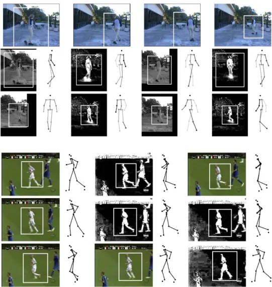
Fig. 4 Circular walking sequence from Sidenbladh et al. (2000). The figure shows full frames (top), and cutouts with bounding boxes in original or segmented input images, as well as stick figures of the estimated body poses. For the visualisation of the 3D stick figures, body limbs that are closer in depth appear darker in the plot

Fig. 5 An extract from a soccer game. The figure shows original and segmented images and with estimated bounding boxes, and estimated 3D poses

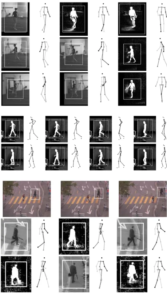
background subtraction, yielding noisy foreground proba-bility maps. The main challenge here is the varying view-ing angle that is difficult to estimate from the noisy silhou-ettes. Figure8shows another publicly available sequence.3 Here we used only one camera, while this sequence has been mainly used for multi-camera tracking (e.g. Sigal et al.2004; Sun et al.2006).

Figure5shows an extract from a real soccer game with a running player. The sequence was obtained from www. youtube.com, therefore the resolution is low and the qual-ity suffers from compression artefacts. We obtained a fore-ground segmentation by masking the colour of the grass.

Figure9shows an extract from a treadmill sequence that was 1660 frames long in total. In this sequence, the subject initially walks and switches to running and back to walking several times. The figure shows a few frames from the tran-sition from running to walking; the first two frames clearly

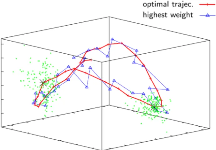
Fig. 6 (Color online) Final trajectory through the LLE pose space ob-tained by the global optimisation step (red curve in the figure). A sub-sequence of 36 frames, roughly one walking cycle, is shown here. The

blue circles correspond to the particles with the highest weight, for

each timestep of the online tracking algorithm. The green dots indicate the sample distribution at frame 4 and 24 of this subsequence

3_{http://www.cs.brown.edu/~ls/}

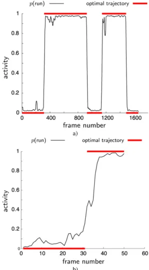
contain running poses, then the arms are lowered and the last 3 frames show walking. The plot in Fig.11a shows the esti-mated running probabilities throughout this sequence. Even for humans, it is not obvious to identify the exact moment of activity change, there is typically a transition phase of about 0.5 seconds. In our experiments, the activity switch was al-ways detected within this transition phase, as desired. Note that we do not take into account the typical periodic motion in vertical direction that distinguishes running from walk-ing, the activity is correctly estimated from the local shape and its deformation over time alone.

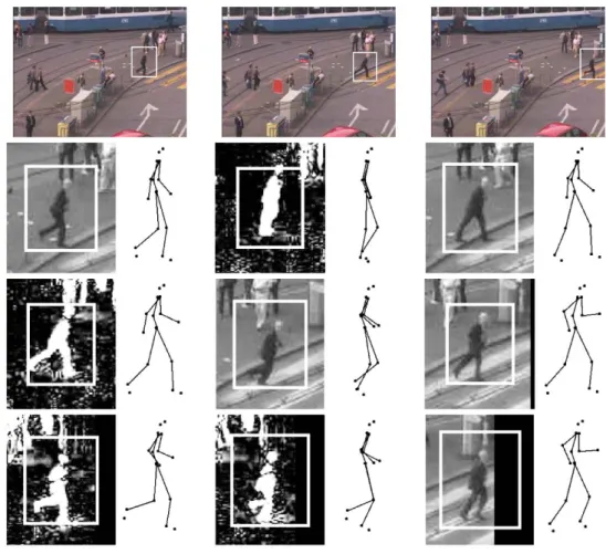
The sequences of Figs.10and12were recorded in a real traffic environment with a webcam. The image resolution is 320×200 pixels, with subjects as small as 40–50 pixels in height. Furthermore, the image quality is unfavourable due to severe MPEG compression artefacts and noisy fore-ground segmentation that was carried out by subtracting one of the frames at the beginning of the sequence. In Fig.10the person carries an umbrella that could be misinterpreted as a leg, and a bag that distorts the overall shape of the pedes-trian. The subject also turns away from the camera over the duration of the sequence. Our experiments showed that such a challenging sequence, combining different kinds of diffi-culties, can only be tracked thanks to the dynamical model, since the information from individual images is unreliable and therefore has to be accumulated over time. The pedes-trian in Fig.12suddenly starts to run when crossing a street. The activity switch is reliably detected, as can be seen in the activity plot in Fig.11b.

6 Discussion

The proposed approach relies on strong models of prior knowledge about typical human motion patterns. This sug-gests its use for image sequences, where this prior knowl-edge is actually needed. For high-resolution multi-camera input sequences, an approach that predominantly relies on the image information might yield more accurate results, and generalise better to unseen motion patterns.

Fig. 7 Graphical model of the Markov chain in which the global optimisation is performed

Fig. 8 Circular walking sequence from Sigal et al. (2004), original resp. segmented input images with estimated bounding boxes, and estimated poses

Fig. 9 Transition from running to walking. The original sequence is 1660 frames long, here we show selected frames from the transition phase between frame 921 and frame 936. See also Fig.11a for a plot of the estimated activity categories of this sequence

Fig. 10 Real traffic scene with low resolution input images, noisy segmentation, disturbing objects (umbrella, bag), and varying viewangle. Original frames (top) and cutouts

Fig. 11 Activity plots of the sequences of Figs.9a and12b. The figures show the estimated activities; the curve shows the continuous proba-bility that we observe running rather than walking over the entire se-quence, the bars indicate the activity label that has been inferred by the global optimisation

The main reasons for failures of the tracking algorithm are excessive noise in the segmented images, especially if the false segmentations are due to occlusions or background objects and thus not randomly distributed. Furthermore, it is very difficult to estimate body poses if the walking direction and view direction of the camera coincide. In such front-views, the image variation that is caused by the body motion is very small, typically much smaller than the image noise, and does thus not allow for successful tracking.

The presented system exhibits complex interactions be-tween its different modules. It would be desirable to evaluate them individually, which is however difficult, because they rely on each other and are often only applicable in combi-nation. For instance, the proposed sampling-based inference scheme requires a low-dimensional pose representation to operate with a moderate number of samples, and so does the learning stage to ensure good generalisation and avoid

overfitting. One module that can easily be switched on or off without altering the overall approach is the dynamical model. Here, we have observed that the challenging traffic sequences of Figs.10and12clearly fail if a simple Brown-ian motion dynamic model is used instead of the learned model. If the images are of low quality and lack detailed shape information, the scissor-like opening and closing of the legs of a walking person might e.g. as well be explained by a backwards walking motion. A low temporal resolution increases the risk of confusion between posterior modes, that can be limited by the dynamical model.

While the activity transition is in general accurately de-tected, the applied transition model is currently very sim-ple. As there are no activity transitions in the training cor-pus, the transition itself is not learned. Instead, the transi-tion behaviour is modelled by incorporating the obvious as-sumption of smooth motion across the activity change, as shown in Sect.3.1. The results show that the algorithm is able to reliably detect an activity switch and to temporally locate it precisely. Furthermore, the tracked body motion shows a smooth transition from one activity into the other and looks natural. As a possible extension of the system, the actual transition phase could be modelled more accurately by learning from training data as well, including additional body postures that are neither walking nor running poses but occur only during the transition phase.

7 Summary and Conclusion

We presented a monocular tracking approach that simul-taneously estimates the 2D bounding box coordinates, the performed activity, and the 3D body pose of a moving per-son. To this end, we learn statistical models of pose, dy-namics, activity transition, and appearance using efficient sparse kernel regressors. The relationship of pose and ap-pearance is learned in a generative manner. Using LLE, we find an embedding of the pose manifolds of low dimension-ality, which allows us to use a Monte-Carlo sampling algo-rithm for tracking. A max-product algoalgo-rithm finally extracts the optimal sequence through the entire image sequence. We demonstrated the method on several challenging video se-quences of low resolution with noisy segmentation.

The activity recognition results reported in this article were nearly perfect, suggesting that the discrimination be-tween the considered activities is a relatively easy task, pro-vided that the tracking works well. Currently, we are apply-ing the proposed method to different data sets with other ac-tivity categories than walking and running. This will allow for more detailed conclusions about the potential of our al-gorithm for the recognition of subtle activity classes. While this article focuses on real-world sequences, a quantitative evaluation of the pose estimation on a benchmark dataset with ground-truth is planned.

Fig. 12 Real traffic scene with a transition from walking to running. Full frames (top) and cutouts with estimated poses. Figure11b shows the inferred activity categories of this sequence

A further line of current research in tracking related ar-eas is the investigation of other appearance descriptors, and methods to extract interesting features from image data in a statistically meaningful way. One goal is to eventually avoid the need for a segmentation of the images. A different strat-egy that will be considered is a deeper integration of image segmentation, 2D tracking and 3D pose estimation, where the interaction between these different stages will be inves-tigated.

Acknowledgements This work is supported, in parts, by the FP6 EU Integrated Project DIRAC (IST-027787), the SNF project PICSEL and the SNF NCCR IM2.

References

Agarwal, A., & Triggs, B. (2004a). 3D human pose from silhouettes by relevance vector regression. In IEEE conference on computer

vision and pattern recognition (CVPR).

Agarwal, A., & Triggs, B. (2004b). Tracking articulated motion using a mixture of autoregressive models. In European conference on

computer vision (ECCV).

Agarwal, A., & Triggs, B. (2005). Monocular human motion capture with a mixture of regressors. In IEEE CVPR workshop on vision

for human-computer interaction.

Bailey, D. G. (2004). An efficient euclidean distance transform. In

In-ternational workshop on combinatorial image analysis.

Bhattacharyya, A. (1943). On a measure of divergence between two statistical populations defined by their probability distributions.

Bulletin of the Calcutta Mathematical Society.

Doucet, A., Godsill, S., & Andrieu, C. (2000a). On sequentional Monte Carlo sampling methods for Bayesian filtering. Statistics and

Computing.

Doucet, A., Godsill, S., & West, M. (2000b). Monte Carlo filtering and smoothing with application to time-varying spectral estimation. In

IEEE conference on acoustics, speech and signal processing (vol.

II, pp. 701–704).

Elgammal, A., & Lee, C.-S. (2004). Inferring 3D body pose from sil-houettes using activity manifold learning. In IEEE conference on

computer vision and pattern recognition (CVPR).

Forney, G. D. (1973). The Viterbi algorithm. Proceedings of the IEEE,

61(3), 268–278.

Forsyth, D. A., Arikan, O., Ikemoto, L., Brien, J. O., & Ramanan, D. (2006). Computational studies of human motion: Part 1.

Com-puter Graphics and Vision, 1(2/3).

Grauman, K., Shakhnarovich, G., & Darrel, T. (2003). Inferring 3D structure with a statistical image-based shape model.

Interna-tional conference on computer vision (ICCV).

Isard, M. (2003). Pampas: Real-valued graphical models for computer vision. In IEEE conference on computer vision and pattern

recog-nition (CVPR).

Isard, M., & Blake, A. (1998a). Condensation—conditional density propagation for visual tracking. International Journal of

Com-puter Vision, 29(1), 5–28.

Isard, M., & Blake, A. (1998b). A mixed-state CONDENSATION tracker with automatic model-switching. In International

Jaeggli, T., Koller-Meier, E., & Gool, L. V. (2006). Monocular tracking with a mixture of view-dependent learned models. In IV

confer-ence on articulated motion and deformable objects (AMDO).

Kschischang, F., Frey, B. J., & Loeliger, H.-A. (2001). Factor graphs and the sum-product algorithm. IEEE Transactions on

Informa-tion Theory, 47(2), 498–519.

Lawrence, N. D. (2005). Probabilistic non-linear principal component analysis with Gaussian process latent variable models. Journal of

Machine Learning Research, 6, 1783–1816.

Lee, C.-S., & Elgammal, A. (2007). Modeling view and posture mani-folds for tracking. In International conference on computer vision (ICCV).

Li, R., Yang, M.-H., Sclaroff, S., & Tian, T.-P. (2006). Monocular tracking of 3D human motion with a coordinated mixture of factor analyzers. In European conference on computer vision (ECCV) (pp. 137–150).

Li, R., Tian, T.-P., & Sclaroff, S. (2007). Simultaneous learning of non-linear manifold and dynamical models for high-dimensional time series. In International conference on computer vision (ICCV). Lim, H., Camps, O. I., Sznaier, M., & Morariu, V. I. (2006). Dynamic

appearance modeling for human tracking. In IEEE conference on

computer vision and pattern recognition (CVPR) (pp. 751–757).

Moeslund, T., Hilton, A., & Krüger, V. (2006). A survey of advances in vision-based human motion capture and analysis. Computer

Vi-sion and Image Understanding, 104(2), 90–126.

Navaratnam, R., Fitzgibbon, A. W., & Cipolla, R. (2007). The joint manifold model for semi-supervised multi-valued regression. In

International conference on computer vision (ICCV).

Pavlovic, V., Rehg, J. M., & MacCormick, J. (2001). Learning switch-ing linear models of human motion. In Neural information

processing systems.

Rosales, R., & Sclaroff, S. (2001). Learning body pose via specialized maps. In Neural information processing systems.

Roweis, S., & Saul, L. (2000). Nonlinear dimensionality reduction by locally linear embedding. Science, 290(5500), 2323–2326. Sidenbladh, H., Black, M., & Fleet, D. (2000). Stochastic tracking of

3D human figures using 2D image motion. In European

confer-ence on computer vision (ECCV) (pp. 702–718).

Sigal, L., Bhatia, S., Roth, S., Black, M., & Isard, M. (2004). Tracking loose-limbed people. In IEEE conference on computer vision and

pattern recognition (CVPR).

Sminchisescu, C., & Jepson, A. (2004). Generative modeling for con-tinuous non-linearly embedded visual inference. In International

conference on machine learning (ICML).

Sminchisescu, C., Kanaujia, A., Li, Z., & Metaxas, D. (2005). Dis-criminative density propagation for 3D human motion estimation. In IEEE conference on computer vision and pattern recognition (CVPR).

Sudderth, E. B., Ihler, A. T., Freeman, W. T., & Willsky, A. S. (2003). Nonparametric belief propagation. In IEEE conference on

com-puter vision and pattern recognition (CVPR).

Sun, Y., Bray, M., Thayananthan, A., Yuanand, B., & Torr, P. (2006). Regression-based human motion capture from voxel data. In

British machine vision conference.

Tenenbaum, J., de Silva, V., & Langford, J. (2000). A global geomet-ric framework for nonlinear dimensionality reduction. Science,

290(5500), 2319–2323.

Thayananthan, A., Navaratnam, R., Stenger, B., Torr, P., & Cipolla, R. (2006). Multivariate relevance vector machines for tracking. In

European conference on computer vision (ECCV).

Tipping, M. (2000). The relevance vector machine. In Neural

informa-tion processing systems.

Urtasun, R., Fleet, D. J., & Fua, P. (2006). 3D people tracking with Gaussian process dynamical models. In IEEE conference on

com-puter vision and pattern recognition (CVPR) (pp. 238–245).

Wang, J. M., Fleet, D. J., & Hertzmann, A. (2006). Gaussian process dynamical models. In Neural information processing systems (pp. 1441–1448).

Wiberg, N. (1996). Codes and decoding on general graphs. PhD the-sis, Department of Electrical Engineering, Linköping University, Sweden.

Yedidia, J., Freeman, W., & Weiss, Y. (2002). Understanding belief

propagation and its generalizations (Technical report

TR-2001-22). MERL.

Zivkovic, Z., & Verbeek, J. (2006). Transformation invariant compo-nent analysis for binary images. In IEEE conference on computer