A two stage Bayesian stochastic optimization model for cascaded hydropower systems considering varying uncertainty of flow forecasts

RESEARCH ARTICLE

10.1002/2013WR015181

A two stage Bayesian stochastic optimization model for

cascaded hydropower systems considering varying uncertainty

of flow forecasts

Wei Xu1,2_{, Chi Zhang}1_{, Yong Peng}1_{, Guangtao Fu}3_{, and Huicheng Zhou}1

1_{School of Hydraulic Engineering, Dalian University of Technology, Dalian, China,}2_{College of River and Ocean}

Engineering, Chongqing Jiaotong University, Chongqing, China,3Centre for Water Systems, College of Engineering, Mathematics, and Physical Sciences, University of Exeter, Exeter, UK

Abstract

model for real time operation of cascaded hydropower systems to handle varying uncertainty of inflow fore-casts from Quantitative Precipitation Forefore-casts. In this model, the inflow forefore-casts are considered as having increasing uncertainty with extending lead time, thus the forecast horizon is divided into two periods: the inflows in the first period are assumed to be accurate, and the inflows in the second period assumed to be of high uncertainty. Two operation strategies are developed to derive hydropower operation policies for the first and the entire forecast horizon using TS-BSDP. In this paper, the newly developed model is tested on China’s Hun River cascade hydropower system and is compared with three popular stochastic dynamic programming models. Comparative results show that the TS-BSDP model exhibits significantly improved system performance in terms of power generation and system reliability due to its explicit and effective uti-lization of varying degrees of inflow forecast uncertainty. The results also show that the decision strategies should be determined considering the magnitude of uncertainty in inflow forecasts. Further, this study con-firms the previous finding that the benefit in hydropower generation gained from the use of a longer hori-zon of inflow forecasts is diminished due to higher uncertainty and further reveals that the benefit reduction can be substantially mitigated through explicit consideration of varying magnitudes of forecast uncertainties in the decision-making process.

1. Introduction

With recent improvements in weather forecasting technologies, there is increasing attention on the use of weather forecasts to improve reservoir operation [e.g.,Niewiadomska-Szynkiewicz et al., 1996;Chang et al., 2005;Hsu and Wei, 2007;Ngo et al., 2007;Saavedra Valeriano et al., 2010a, 2010b]. Weather forecasts are generally available at different time scales, for example, nowcasts (0–6 h), short range forecasts (1–3 days), and medium range forecasts (3–10 days), which are related to different degrees of predictive accuracy. Short range Quantitative Precipitation Forecasts (QPFs) have long been used for water system management, for example, real time flood control [e.g.,Niewiadomska-Szynkiewicz et al., 1996;Hsu and Wei, 2007;Ngo et al., 2007;Saavedra Valeriano et al., 2010a, 2010b] and short term hydroelectric system operation [Zhou et al., 2005;Wang et al., 2005]. Although medium range QPFs have a reduced accuracy and reliability com-pared to short range QPFs, they have been proven to be useful for reservoir operation [Collischonn et al., 2005, 2007;Bravo et al., 2009;Tang et al., 2010]. For example, medium range QPFs have been used to fore-cast reservoir inflow for hydroelectric system operation [e.g.,Zhou et al., 2005;Wang et al., 2005;Collischonn et al., 2007;Zhou et al., 2009, 2010;Tang et al., 2010] and interbasin water transfer operation [e.g.,Liang et al., 2009,Wang et al., 2010;Xi et al., 2010]. At the same time, the limitations of use of these forecasts have been highlighted due to high levels of predictive uncertainty [Meneguzzo et al., 2004;Bartholmes and Todini, 2005]. Uncertainty in QPFs is a major factor affecting the accuracy of inflow forecasts and thus the develop-ment of reservoir operating policies [Roulin and Vannitsem, 2005;Mascaro et al., 2010;Saavedra Valeriano et al., 2010b]. Thus, effectively addressing uncertainties in QPFs is critical to support informed decision mak-ing of reservoir operation [Cui et al., 2011;Fan and van den Dool, 2011]. This study will investigate the explicit use of varying magnitudes of uncertainty in QPFs to improve the performance of cascaded hydro-power systems, which, to the best of our knowledge, has not been attempted in the literature.

Key Points:

Two stage BSDP is developed

Considering varying levels of forecast uncertainty improves performance

Benefit reduction from use of longer inflow forecasts is mitigated

Correspondence to:

C. Zhang, [email protected]

Citation:

Xu, W., C. Zhang, Y. Peng, G. Fu, and H. Zhou (2014), A two stage Bayesian stochastic optimization model for cascaded hydropower systems considering varying uncertainty of flow forecasts,Water Resour. Res.,50, 9267–9286, doi:10.1002/

2013WR015181.

Received 16 DEC 2013 Accepted 2 OCT 2014

Accepted article online 7 OCT 2014 Published online 9 DEC 2014

Water Resources Research

Stochastic Dynamic Programming (SDP) has been used to develop reservoir operation policies with the con-sideration of inflow uncertainties.Dutta and Houck[1984] andDutta and Burges[1984] assumed that the distribution of forecast uncertainties remains unchanged during the entire forecast horizon. The efficiency and reliability of hydropower operation are substantially affected by the assumption of forecast uncertain-ties [Tejada-Guibert et al., 1995]. In order to reduce the negative influence on decision making caused by high inflow uncertainty in a long forecast horizon (FH),Stedinger et al. [1984] suggested to employ only the best inflow forecasts within the beginning period of FH and discard the inflow forecasts in the remaining periods of FH with the intent of deriving improved reservoir operating policies. Recent research demon-strated that uncertainty in QPFs and inflow forecasts generally increases with an extending lead time [ Simo-novic and Burn, 1989;Maurer and Lettenmaier, 2003, 2004;You and Cai, 2008;Zhao et al., 2012]. To

effectively quantify inflow forecast uncertainty,Karamouz[1990] suggested the use of Bayesian decision theory to interpret inflow uncertainty by incorporating new information associated with inflow probabilities. Further, a Bayesian Stochastic Dynamic Programming (BSDP) model was developed by embedding Bayesian theory in SDP to represent inflow uncertainty [Karamouz and Vasiliadis, 1992].Kim and Palmer[1997] used a BSDP model to investigate the potential benefits of using seasonal flow forecasts in hydropower generation. Mujumdar and Nirmala[2007] aggregated individual inflows of reservoirs in a cascaded hydropower system, and represented the forecast uncertainty of the aggregated inflow using a BSDP model.Zhou et al. [2009] andTang et al. [2010] proposed a hybrid method that employs a SDP model for dry seasons and BSDP model for wet seasons. On one hand, increasing FH may provide more information for decision making in a longer time framework, on the other hand the benefit gained from a longer horizon may be offset by increasing forecast uncertainty [You and Cai, 2008;Zhao et al., 2012]. However, in the BSDP models men-tioned above, inflow forecast is treated as having the same level of uncertainty over the entire FH and the varying magnitudes of uncertainty are not explicitly considered for the development of reservoir

operations.

The primary purpose of this paper is to present a new Two Stage Bayesian Stochastic Dynamic Program-ming (TS-BSDP) methodology for real time operation of cascaded hydropower systems. The newly pro-posed methodology in this study consists of a new Bayesian method which uses inflow forecasts for real-time reservoir operation in a more effective way, and also an aggregation-disaggregation approach that allows the proposed method to be implemented for a complex hydropower system in a more efficient way. To utilize the varying magnitudes of uncertainty in inflow forecasts with a medium-range forecast horizon, this methodology partitions the forecast horizon into two periods and consequently two different strategies are developed to incorporate the inflow uncertainties of the two periods through Bayesian theory for reser-voir operation. The two strategies are designed to investigate the best way to utilize forecast inflows with different magnitudes of uncertainty in the two periods; they also allow for comparison of the impacts of dif-ferent lengths of decision horizon on system performance regarding hydropower generation and reliability. Further, an aggregation-disaggregation approach is used to reduce the dimensional complexity of cascaded reservoir operation problems. The newly developed methodology is demonstrated using the Hun River cas-caded hydropower reservoirs in China.

2. Two Stage Bayesian Stochastic Optimization Model

For multireservoir systems, the SDP and BSDP models become computationally intractable due to the curse of dimensionality problem, thus simplification is usually needed. An aggregation approach has been used to improve computational efficiency, in which a multireservoir system with cascaded hydropower stations is simplified as a single virtual reservoir through aggregation of the storage and inflow of individual reser-voirs [Turgeon, 1980;Turgeon and Charbonneau, 1998;Valdes et al., 1992;Liu et al., 2009].Hall and Dracup [1970] originally aggregated the storages of all reservoirs in a hydropower system into an equivalent reser-voir to solve the dimensionality problem of deterministic dynamic programming, and optimal policies for the aggregated reservoir were decomposed into individual policies for each reservoir through the pre-scribed relationships between the reservoirs. An energy-based approach was later developed for decompo-sition by converting the inflows and storages of individual reservoirs to the potential energy available, which can be taken as a state variable to handle the nonlinear relationship between the volume of water release and the power generated [Turgeon, 1980;Turgeon and Charbonneau, 1998;Liu et al., 2011]. However, the energy approach did not consider the individual characteristics of the reservoirs and the amount of

water to be released from the aggregated reservoir [Archibald et al., 2006]. An alternative approach was pro-vided to construct the relationship between the state variables of individual reservoirs using historical data [Saad et al., 1994;Ponnambalam and Adams, 1996;Archibald et al., 1997, 2006;Serrat-Capdevila and Valdes, 2007]. In the optimization process, the aggregate variables are disaggregated to estimate the optimal objec-tive value according to the relationship. In this study, the conditional expectation method, developed by Loucks et al. [1981], is selected as the disaggregation model. The conditional expectation method has been successfully applied to disaggregate the aggregate inflow for cascaded hydropower reservoirs byMujumdar and Nirmala[2007].

Building on the aggregation-disaggregation concept described above, the TS-BSDP model is developed in this study. This model is compared with the following three models: the Aggregate Flow Stochastic Dynamic Programming (AF-SDP), the Aggregation-Disaggregation Stochastic Dynamic Programming (AD-SDP) and the Aggregation-Disaggregation Bayesian Stochastic Dynamic Programming (AD-B(AD-SDP). The AF-SDP considers only the aggregation of individual reservoir inflows, and a single equivalent reservoir is not constructed. The other models consider the aggregation of both inflows and storages, and simplify the hydropower system to a single virtual equivalent reservoir for optimization. The aggregate storage and inflow are decomposed into values for each reservoir based on the storage-discharge relationships derived using historical data.

In this section, the aggregation-disaggregation approach is first introduced to construct a virtual equivalent reservoir. The uncertainties of the aggregate inflow are then addressed using Bayesian theory. Finally the structure and recursive equations of the TS-BSDP model are introduced.

2.1. Aggregation-Disaggregation Approach 2.1.1. Construction of an Equivalent Reservoir

The single equivalent reservoir is constructed by aggregating the inflows and storages of individual reser-voirs to reduce the complexity of the optimal reservoir operation problem. The aggregate inflow is used as a state variable, and is calculated asQt5

XZ

z51q

z

t, whereqzt is the inflow of reservoirzat time steptandZ

is the total number of reservoirs. The aggregate inflow is discretized into a number of adjoining intervals, each of which is represented by an element in the set Q1

t; ;Q

l

t

, wherelis the total number of discreti-zation levels.

According toMujumdar and Nirmala[2007], the AF-SDP model aggregates only the inflows of the individual reservoirs. The storages of individual reservoirs are discretized into a number of adjoining intervals, repre-sented by the elements in the set mz

1; ;mzbz

n o

, wherebzis the number of storage intervals for reservoirz. The number of possible combinations of storage intervals of individual reservoirs isb13 3bz. Thus the AF-SDP model can result in the curse of dimensionality problem when the number of reservoirs or/and number of storage discretizations are large.

Apart from AF-SDP, all other models used in this study consider aggregation of the storages of individual reservoirs. The minimum and maximum reservoir storages of the equivalent reservoir are represented by

Vmax5 XZ z51 v_maxz Vmin5 XZ z51 vz min 8 > > > > > < > > > > > : (1) wherevz

min andvzmaxrepresent the minimum and maximum storages of reservoirz, respectively. The

equiv-alent reservoir storage is discretized into adjoining intervals, which are represented by V1; ;V/

, where the subscript/is the number of storage discretizations.

2.1.2. Disaggregation of Aggregate Variables

Once the optimal problem is solved based on the equivalent reservoir, the aggregate variables (inflow and storage) have to be disaggregated to the relevant variables of each individual reservoir. The conditional expectation method is used for disaggregation in this study [Loucks et al., 1981;Mujumdar and Nirmala 2007]. When aggregate variableRtat time steptbelongs to intervalr, the conditional expectation of the

related variable for reservoirz(denoted byRz

Rz_t5fðRz_tjR_tÞ5E R z_tjRt5r5X nt iz51 P R _tz5izjRt5rnr_izt5X nt iz51 P_rizt nr_izt (2)

whereizrepresents an interval ofRz

tfor reservoirz;ntis the number of intervals (iz) at time stept;nrizt is the

expected value ofRz

tin intervaliz;Ptrizrepresents the probability that individual variable (Rzt) at time stept

belongs to the intervaliz, given the aggregate variable (Rt) at time steptbelongs to intervalr.

The inflow of each individual reservoir at time stept, represented usingqz

t(z51,. . .,Z), can be calculated

by replacing the variables in equation (2) with relevant flow variables. Similarly, the storages at the begin-ning and end of time stept, i.e.,sz

t21andszt (z51,. . .,Z), can also be calculated.

With the equivalent reservoir, the optimization problem is solved by taking the aggregated inflow and storage as state variables. In developing the operation policies of the equivalent reservoir, the decision variables are converted to the aggregate output. The aggregate output is then disaggregated with the objectives of minimizing the spillages and maximizing the amount of water at the end of the operation period as below:

FtðhtÞ5max fendlevðhdtjst21;qt;HtÞ2gfspillðhdtjst21;qt;HtÞ

d2D (3)

wherefendlevðhdtjkt;qt;HtÞandfspillðhdtjkt;qt;HtÞare the functions of storage at the end of time steptand

spillage at time stept, respectively.Htis the aggregate output obtained according to operation policies.hdt

is thedth output combination of individual reservoirs by disaggregatingHtat time stept.Dis the total

number of combinations.htis the output combination, which is selected for operation.st21is the storage

combination of individual reservoirs at beginning of time stept, andqtis the inflow of individual reservoirs

at time stept.gis a penalty factor, typically in the interval [1, 10], and is used to direct the search to reduce the overall spillage from all reservoirs [Tang et al., 2010].

2.2. Uncertainties of Aggregate Inflow

In a simple SDP model, the reservoir inflow is normally represented using a simple Markov process. The ran-domness of the inflow at time stept11 is addressed through a prior inflow transition probabilityP Q½ t11jQt,

given inflowQtat time stept.

In a BSDP model, the inflow forecast uncertainty at time steptis represented in equation (4) using the pos-terior inflow transition probabilityP Q½ tjFt;Qt21, given the observed inflow (Qt21) at time stept-1 and inflow

forecast (Ft) at time stept. The predictive probability of forecasts is represented byP F½ t11jQt, as described

in equation (5) below. P Q½ tjFt;Qt215 P F½ tjQt3P Q½ tjQt21 X Qt P F½ tjQt3P Q½ tjQt21 (4) P F½ t11jQt5 X Qt11 P F½ t11jQt113P Q½ t11jQt (5)

2.3. Optimization Problem Formulation 2.3.1. Objective Function

The operation policy in this study is to maximize the total power production as well as to minimize the devi-ation from the required system output to guarantee the stability of power supply. Thus, the objective func-tion consists of two components: power producfunc-tion and penalty for deviafunc-tion from system requirements as below ftðst21;qtÞ5max XT t51E B½ ðst21;qt;stÞ n o 8st21;qt;st where Bðst21;qt;stÞ5 bðst21;qt;stÞ2a½maxðe2bðst21;qt;stÞ;0Þb n o Dt (6)

whereftðÞrepresents the maximum expected hydropower generation for the entire planning horizon (T)

andt51; ;T.bðÞ(MW) is a function of power generation given storage variablesst21andstat the

begin-ning and end of time steptand flow variableq_tat time stept, andeis the required firm output, which is 76 MW for the case study.aandbare penalty factors;Dt(h) is decision interval.

2.3.2. State and Decision Variables

In this study, there are four models with different variables considered. In AF-SDP, the aggregate inflow at time steptand storage combination of individual reservoirs at the beginning of time steptare taken as state variables, and the storage combination of individual reservoirs at end of time steptis taken as a deci-sion variable. In AD-SDP, the aggregate inflow at time steptand aggregate storage of the equivalent reser-voir at the beginning of time steptare taken as state variables, and the aggregate storage at the end of time steptis taken as decision variable. In addition to the variables in AD-SDP, AD-BSDP considers the aggregate inflow at the previous time stept21 as an additional state variable. While in TS-BSDP, the aggre-gate inflow at time steptis partitioned into two periods. Thus the state variables are aggregate inflows of two periods and aggregate storages at the beginning of time stept, and the decision variable is aggregate storage at the end of time stept.

2.4. Decision Strategies and Recursive Equations 2.4.1. Decision Strategies

It is important to determine the decision horizon in terms of the FH in the reservoir operation optimization problems. Figure 1a describes a general decision-making strategy in which the inflow forecast in the entire FH is used to determine the operation policies in the same period. This strategy is defined as Strategy A. This strategy is employed by AF-SDP, AD-SDP and AD-BSDP models in this study. In this way, the inflow forecast uncertainties in the entire horizon are treated identically. The longest FH available in this study is 10 days. Two cases with different time steps are used for comparison of the different models, i.e.,t55 or 10 days. In TS-BSDP model, the entire inflow FH (10 days) is partitioned into two periods: Short-range Forecast (SF, 1–5 days) and Medium-range Forecast (MF, 6–10 days). The time steptis 5 days in this model and two decision-making strategies, shown in Figures 1b and 1c, are developed to compare the impacts of different lengths of decision horizon on system performance. Figure 1b shows Strategy B, which uses the inflow fore-casts at time stepstandt11 to determine the operation policies for time stept. Figure 1c shows Strategy C, which uses the inflow forecasts at time stepstandt11 to determine the operation policies for time steps tandt11.

2.4.2. AF-SDP Model Recursive Equation

The AF-SDP model takes the storages of individual reservoirs and the aggre-gate inflow as state variables. In this model, the randomness of aggregate inflow for forecast horizons of 5 days and 10 days are depicted in Figures 2a and 2b respectively. The randomness of inflow is addressed by the prior inflow transition probabilityP Q½ t11jFt

(denoted byPt

ij), where the subscripti

represents theith interval of aggre-gate inflow forecast (Ft) att, andj

rep-resents thejth interval of aggregate inflow (Qt11) att11. The recursive

equation is defined below

t+1 t FH DH (a) t t+1 SF MF DH (b) t t+1 SF DH MF (c)

Figure 1.Three different decision-making strategies used by the four models. DH and FH represent decision horizon and forecast horizon,

respectively. a t-1 t t+1 Qt Qt+1 Qt-1 5 t

F

P

F

P

F

F

Figure 2.Representation of inflow uncertaintiesof various models. (a) and (b) SDP;

ftðst21;iÞ5maxst Bðst21;i;stÞ1RjP t

ijft11ðst;jÞ

h i

(7) whereftðst21;iÞrepresents the maximum expected hydropower generation from time stepttoT.

2.4.3. AD-SDP Model Recursive Equation

Recall that a single equivalent reservoir is constructed to reduce the dimension of the optimal reservoir operation problem in AD-SDP model. Thus, the AD-SDP model uses both the aggregate storage and aggre-gate inflow as state variables. Comparing AD-SDP and AF-SDP can reveal the efficiency in the use of the equivalent reservoir in the optimization process.

Assuming thatSt21andStrepresent the aggregate storages at the beginning and end of time stept, these

variables are disaggregated using the method of conditional expectation, i.e., equation (2). The recursive equation is defined as ftðSt21;iÞ5maxSt BðSt21;i;StÞ1RjP t ijft11ðSt;jÞ h i (8) whereirepresents the interval of inflow forecast (Ft) at time stept, andjrepresents the interval of

aggre-gate inflow (Qt11) att11.

2.4.4. AD-BSDP Model Recursive Equation

In AF-SDP and AD-SDP, the randomness of aggregate inflows is addressed as a simple Markov Process; the inflow forecasts are considered as accurate information. In the BSDP model, however, the inflow forecast uncertainty is addressed by Bayesian theory. Comparing the performance of AD-SDP and AD-BSDP, the impact of inflow forecast uncertainties on decision making can be evaluated.

Figures 2c and 2d show how the inflows are updated for two forecast horizons, i.e., 5 days and 10 days, respectively. ThePt

hikrepresents the posterior flow transition probability (P Q½ tjFt;Qt21);Ptknrepresents

pre-dictive probability of inflow forecasts (P F½ t11jQt). The recursive equation for AD-BSDP is defined as ftðSt21;h;iÞ5maxSt RkP

t

hikBðSt21;k;StÞ1RnPknt ft11ðSt;k;nÞ

(9) wherehrepresents the interval of inflow (Q_t-1) at time stept-1;irepresents the interval of inflow forecast (Ft) at time stept;krepresents the interval of inflow (Qt) at time steptandnrepresents the interval of

inflow forecast (F_t11) at time stept11.

2.4.5. TS-BSDP Model Recursive Equation

Although AD-BSDP considers the inflow forecast uncertainties, they are treated indifferently across the entire FH. Thus, the TS-BSDP model is constructed to explicitly utilize the varying magnitudes of inflow fore-cast uncertainty and make the best of the information available to improve system performance.

Figure 2e shows the representation of inflow uncertainties in TS-BSDP. The inflow forecast horizon (10 days) is partitioned into two parts equally: the inflow forecasts in SF (1–5 days) are assumed to be accurate. The forecast uncertainties in MF (6–10 days) are addressed by Bayesian theory. It should be noted that similar to AF-SDP and AD-SDP inflow forecast in SF is assumed to be accurate. Note that the errors involved in Stage 1 can be propagated into Stage 2 and eventually affect the reservoir operation decisions. However this depends on the length of the first stage. In this particular case study, preliminary investigations showed that there is little benefit of considering the uncertainties in SF in terms of improving system performance. This is due to the relatively high accuracy of inflow forecasts in SF since the length (5 days) of the first period allows a quite accurate forecast in the study area [Chu et al., 2010]. Future work remains for the cases with a long period for Stage 1 where the errors may have a considerable impact.

A backward recursive relationship is developed starting from the final time stepT.fSF

t ðÞ,ftMFðÞandftFHðÞ

are used to represent the maximum expected generation of hydropower for the SF, the MF and the entire FH, respectively. An inflow forecast interval in SF and MF are represented bysandm, respectively. The oper-ation policies of decision Strategies B and Strategy C are derived fromfSF

t ðÞandftFHðÞrespectively. The

recursive equations for different time steps are described below.

When t5T: Since there is no forecast for the MF at time stepT, which is represented asu, a null value. In order to compare the performance at time stepT, the aggregate storages at the end of time stepTis set to Lmin, which is the minimum reservoir storage of the equivalent reservoir. The value ofLmin does not affect

the optimization results when the iteration reaches a steady state. So the recursive equation of MF is equal to that of SF. fSF T ðST21;s;uÞ5max½BðST21;i;LminÞ fMF T ðST21;s;uÞ5max½BðST21;i;LminÞ ( (10)

When t5T-1: When the backward recursion moves one step backward tot5T-1, there are two periods for calculation:T-1 andT. The system performance measure isBðST22;s;ST21Þat the current time stept5T-1.

The expected value of system performance for SF at time stepT-1 is determined by the performance mea-sure at time stepT-1 and the expected value of system performance for SF at time stepTas well as inflow transition fromstok, given the inflow forecasts (s) and (m) at SF and MF, respectively, updated by the posterior flow transition probability (PT

smk). The expected value of system performance for MF atT-1 is

determined by the posterior flow transition probability (PT

smk) and the expected value of the system

per-formance for SF at time stepT. The system performance measure of the entire FH at time stepT-1 is deter-mined by the system performance and inflow forecast of SF and MF. The recursive equation of SF, MF and FH are defined below.

fSF T21ðST22;s;mÞ5max BðST22;s;ST21Þ1PkPTsmkfTSFðST21;k;uÞ fMF T21ðST22;s;mÞ5maxPTsmkfTSFðST21;k;uÞ fFH T21ðST22;s;mÞ5 s s1mf SF T21ðST22;s;mÞ m s1mf MF T21ðST22;s;mÞ 8 > > > > < > > > > : (11)

When tT-2: When the iteration moves backward toT-2 or beyond, there are at least two periods that should be considered for calculation. The expected value of the system performance for SF at time steptis determined by four factors: system performance measure of SF at time stept BðSt21;s;StÞ, the expected

value of system performance for SF at time stept11, the posterior flow transition probability (Pt11

smk) and

the predictive probability of forecasts (Pt11

kn ), which represents the predictive probability of inflow forecasts P F½ t12jQt11wherekrepresents the interval of inflowQt11at time stept11 andn represents the interval of

inflow forecast Ft12at time step t12.The expected value of system performance for MF is determined by the

last three terms. Thus, the recursive equations of SF, MF and FH are defined below. fSF t ðSt21;s;mÞ5max BðSt21;s;StÞ1PkPt 11 smk3 P nPt 11 kn ftSF11ðSt;k;nÞ fMF t ðSt21;s;mÞ5max Ptsmk113 P nPtkn11ftSF11ðSt;k;nÞ fFH t ðSt21;s;mÞ5 s s1mf SF t ðSt21;s;mÞ1 m s1mf MF t ðSt21;s;mÞ 8 > > > > < > > > > : (12)

3. Case study

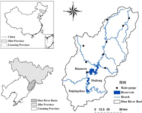
3.1. Hun River Cascade Hydropower Reservoirs

The Hun River cascaded hydropower reservoir system is used to test the newly developed methodology in this study. It is located in the lower reaches of the Hun River basin in the northeast of China. Figure 3 shows the location of the hydropower reservoirs and gauging stations. The basin covers 4040042150N and 124430126500E with an approximate area of 15,000 km2. Precipitation in dry and wet seasons varies sig-nificantly. The mean annual rainfall is about 860 mm, and about 70% to 80% of the precipitation occurs in the wet seasons (from May to September).

Three reservoirs, Huanren, Huilong and Taipingshao, constitute the Hun River cascaded hydropower system and their basic characteristics are listed in Table 1. The upstream reservoir, Huanren reservoir, is the main water source for hydroelectric production. The downstream reservoirs of Huilong and Taipingshao are daily regulation reservoirs. During operation, the Huilong reservoir is most prone to spillage due to its limited regulation ability and small installed capacity.

In the case study, the operator needs to plan the hydropower generation operation policies for the electrical power grid system for 5 days, 10 days, 20 days and a month ahead respectively. In order to guarantee the stability of the electrical power grid system, the operation policies can only be changed at least 5 days ahead, during the normal operating periods except flood periods.

3.2. Forecasted and Observed Data

The Global Forecast System (GFS) developed by the U.S. National Centers for Environmental Prediction, is a global Numerical Weather Prediction (NWP) computer model. The QPFs used in this study are derived from the precipitation forecasts over the entire East Asia region. For research purposes, the GRIB1 data sets are collected from the NOAA server from 2001 to 2010. The QPFs for the 10 days forecast made at the first data assimilation cycle of 0000 UTC every day have been extracted from the GRIB1 data sets for all gauging sta-tions of the Hun river basin shown in Figure 3, by a GRIB1 encoder/decoder program. Finally, the average forecasts of precipitation in the Hun river basin are estimated by the Thiessen polygon method [McCuen, 1998].

The observed precipitation data are available from 1968 to 2010 in the upstream of Huanren. The observed inflow data of each reservoir were obtained from 1968 to 2010. The observed data are used to calibrate and verify the inflow forecasting models.

3.3. Rainfall-Runoff Models

Many hydrological models can be used to predict reservoir inflows using QPFs, such as conceptual rainfall-runoff models and distributed hydrological models [Nijssem et al., 1997;Collischonn et al., 2005, 2007;Tang et al., 2007]. In the case study catchment, the inflow is low and stable during dry seasons (from October to April), however, it becomes high and unstable due to frequent, heavy rainfall during wet seasons (from May to September). Thus, the inflows in this case study are predicted using two models: a multiple linear regres-sion model for dry seasons and Xinan-jiang model for wet seasons, with the intent of improving predictive accuracy.

The multiple linear regression model is based on the correlation relationship between a number of important basin factors and inflow forecasts. Building on previous studies [Liang et al., 2009; Zhou et al., 2010;Tang et al., 2010; Wang et al., 2010], four factors, i.e.,

Figure 3.The Hun River cascade reservoirs system.

Table 1.Characteristics of Hun River Cascaded Hydropower Reservoirs

Characteristic Huanren Huilong Taipingshao

Basin area (km2 ) 10400 2100 528 Total storage (Mm3) 3460 123 182 Usable storage (Mm3 ) 2199 90 164 Dead storage (Mm3 ) 1380 72 145

Normal water level (m) 300 221 191.5

Dead water level (m) 290 219 190

Installed capacity (MW) 222 72 161

Firm output (MW) 33 18 25

Turbine capacity (m3

precipitation and soil moisture of the current period, average inflow of the previous period, and QPFs of the next period, are selected to forecast the inflow at the next period (forecast horizon). The data of soil mois-ture are obtained through continuous simulation using observed daily inflow and precipitation. The param-eters of the multiple linear regression model are determined using the least squares technique [Tang et al., 2010;Wang et al., 2010].

The Xinanjiang model is a conceptual rainfall-runoff model, which was developed byZhao[1992]. This model has been widely used in China, particularly in humid and semihumid regions [e.g.,Cheng et al., 2006]. The inputs to the model are daily precipitation from QPFs and soil moisture indices, and the model output is daily runoff. A Genetic Algorithm (GA) is used to calibrate the Xinanjiang model parameters [Cheng et al., 2006]. The Nash–Sutcliffe Efficiency (NSE) and Root Mean Square Error (RMSE) are used to assess pre-dictive accuracy of the two chosen models.

The inflow forecasting models introduced above were applied to estimate the average inflow for SF (days 1–5), MF (days 6–10) and FH (days 1–10). The respective parameters of the Xinanjiang model and regression model were calibrated against observed data from 1968 to 2000, and were verified with observed data from 2001 to 2010. Based on the calibrated models, the medium-range QPFs of GFS from 2001 to 2010 were applied to forecast the inflows, which were used to assess the performance of the newly developed TS-BSDP model against other SDP models described above. It should be noted that due to the availability of QPF forecasts the performance of the new model discussed above is calculated using the 10 year QPF data, which is used to derive the operational rules. Thus, its performance should be further tested on more hydro-power systems with different system characteristics and different sets of QPF data.

Figure 4 shows the simulated versus observed flows of Huanren reservoir during calibration, verification and forecasting periods. During the periods of calibration and verification, the flow forecasting models perform well, and the values of NSE equal to or greater than 0.9. During forecasting periods, the value of NSE is reduced to 0.77 for the 10 days forecasts. The accuracy for SF is high, with a NSE value of 0.87. But for MF the

value of NSE is only 0.56. The forecasts for high flows, larger than 1000 m3_{/s, are generally lower than the}

observed inflows mainly because high QPFs are generally underestimated, i.e., lower than observed precipita-tions. This clearly shows that the inflow forecasts of SF and MF have different degrees of uncertainty, and thus should have different strategies for use in reservoir operation.

4. Results and Discussion

4.1. Operation Policies

Operation policies from various models are derived using relevant backward recursive equations by iterat-ing until the enditerat-ing storage reaches a steady state [Su and Deininger, 1972;Serrat-Capdevila and valdes, 2007;Mujumdar and Nirmala, 2007], with inflow data from 1968 to 2010. The penalty factors ofaandbin the objective function are set to 1 and 2 respectively, according toTang et al. [2010]. The penalty factor ofg

in equation (3) is set to 5 from the interval [1, 10] through trial and error in terms of the performance of disaggregation.

In the optimization process, the aggregate inflows are discretized into 6 intervals (l56), representing 15%, 30%, 45%, 60%, 75% and 90% percentiles. In AF-SDP model, the storages of Huanren, Huilong and Taiping-shao are discretized into 25, 3 and 3 intervals respectively (b1525;b253;b353). The number of possible combinations of storage is 2533335225. In other models where an equivalent reservoir is constructed, the storage of the equivalent reservoir is discretized into 30 intervals (/530) with an increment of 30 Mm3, resulting in a total number of storage combinations 3033335270. It should be noted that a higher level of discretization can be used for reservoir inflow and storage; however, it might become impractical when coming to real time reservoir operations in practice, as it results in a large number of operating policies for a multireservoir system.

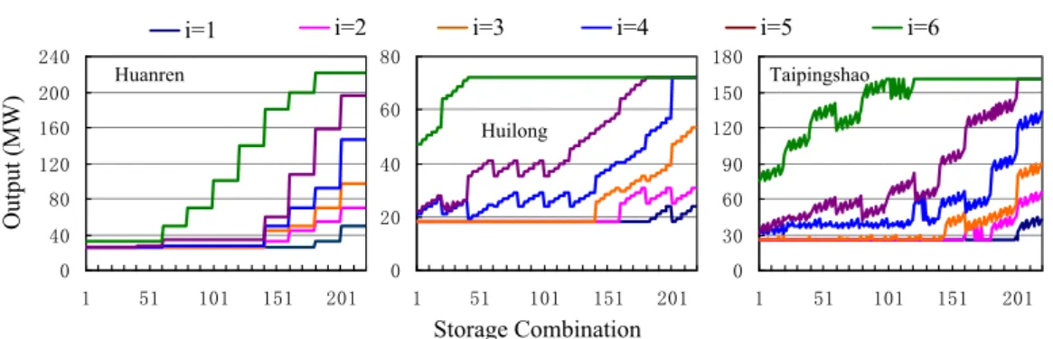
4.1.1. Operation Policies of AF-SDP

Figure 5 shows the operation policies for 10 days derived using the AF-SDP model at time step 22 (from 1 to 10 August). In order to simplify the operation policies, the combinations of individual storages are represented

by numbers, as shown in Table 2. Thus, thexaxis represents the number of storage combinations and yaxis represents the output of individual reservoirs. The different curves represent the results of different intervals (i) in which aggregate inflow forecast lies. The variable ofirepresents the forecasting aggre-gate inflow in current period.

Figure 5 can be interpreted using an operation con-dition as an example, where the storages of Huan-ren, Huilong and Taipingshao are 1380, 90 and 155 Mm3respectively and the aggregate inflow belongs to the 6th interval. The storage combina-tion (1380/90/155) is represented by the number of 8 as shown in Table 2. The outputs of Huanren,

Figure 5.The operation policies derived using AF-SDP.

Table 2.Order Numbers of the Combinations of Storage

Number Storage Combination (Mm3 ) (HR/HL/TPS)a 1 1380/72/145 2 1380/72/155 3 1380/72/164 4 1380/81/145 5 1380/81/155 6 1380/81/164 . . .. . . .. . . 223 2199/90/145 224 2199/90/155 225 2199/90/164 a

HR, HL, and TPS represent the storage of Huanren, Huilong and Taipingshao respectively.

Huilong and Taipingshao for the FH of 10 days are obtained directly from the individual operation poli-cies as 37 MW, 52 MW and 85 MW, respectively.

It can be noted that there are some fluctuations in the output curves of Huilong and Taipingshao, which are caused by the ordering of stor-age combination. As shown in Table 2, the order of reservoirs is Huanren, Huilong, and Taipingshao; this results in the highest level of fluctuation for the last reservoir— Taipingshao, followed by Huilong.

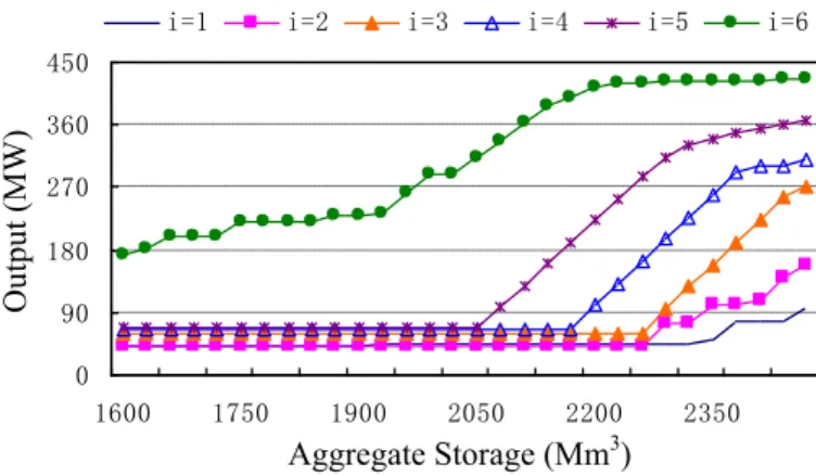
4.1.2. Operation Policies of AD-SDP

Figure 6 shows the operation policies from AD-SDP for 10 days from 1 to 10 August. Recall that the AD-SDP model uses the aggregated inflow and storage of the equivalent reservoir as state variables and the deci-sion variable is converted to the aggregate output of equivalent reservoir. Thus, thexaxis represents the storage of the equivalent reservoir, and theyaxis represents the aggregate output.

Taking the same example as in AF-SDP, the storages of Huanren, Huilong and Taipingshao are 1380, 90, and 155 Mm3respectively and the aggregate inflow belongs to the 6th interval. Recall that the outputs of individ-ual reservoirs, are 37 MW, 52 MW and 85 MW respectively, using the operation policies of AF-SDP in Figure 5. These outputs are expected values, which are the optimal policies for the entire planning horizon (T) under the conditional expectation of inflows instead of the optimal policies for every combination of inflows. Hui-long reservoir has the least regulation potential due to its design storage, so it is most prone to spillage. How-ever, in AF-SDP, the release of Huanren is not controlled to avoid or reduce the spillage at Huilong. While in AD-SDP, the outputs of individual reservoirs are obtained as 33 MW, 60 MW and 88 MW for Huanren, Huilong and Taipingshao, respectively, from the aggregate output of the equivalent reservoir (181 MW). It can be seen that the performances of Huilong and Taipingshao are improved while the performance of Huanren is reduced as a result of reduced release from Huanren. In this way, the performance of AD-SDP is better than that of AF-SDP by storing more water in Huanren reservoir for hydropower generation.

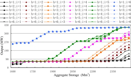
4.1.3. Operation Policies of AD-BSDP

Figure 7 shows the policies derived by AD-BSDP for 10 days from 1 to 10 August. Thexaxis andyaxis have the same meaning as those in Figure 6. In Figure 7,handirepresent the observed inflow (h) at the previous time step and the forecasting inflow (i) at the current time step. The operation policies of AD-BSDP include 36 inflow scenarios. In real-time operation at August 1, the aggregate output for the next 10 days can be obtained according to inflow information ofhandias well as the aggregate storage on 1 August. Comparing the policies in Figures 6 and 7, it can be seen that the operation policies derived by AD-BSDP are affected by observed inflows at the previous time step. For the same inflow forecast intervals in Figure 6, there are six different policy scenarios (represented byh) due to different inflows at the previous time step in Figure 7. The observed inflows at the previous time step are used to reduce the uncertainty of inflow forecast. It can be seen that with an increase in inflow forecast (fromi51 to 6), the influence of the

observed inflows is diminished, with no difference between the six policy scenarios (h51,. . ., 6) wheni56. The results also demonstrate that the observed inflows at the previous time step have a substantially more significant effect in the cases of high storage than low storage, as revealed by the different trajectories at the high storage end in each inflow forecast case in Figure 7.

In comparison with AD-SDP, AD-BSDP addresses the uncertainty of inflow forecast. When the inflow forecast at current time step is high or the reservoir storage is high, the reservoir is prone to spillage. This informa-tion is used for disaggregainforma-tion to avoid or reduce spillage. As a result, the aggregate output of AD-BSDP is larger than that of AD-SDP. Using the same operating example, i.e., when inflow forecasti56 and aggregate

storage is 1600 Mm3, the output from AD-BSDP is 250 MW, representing a significant increase compared to 181 MW from AD-SDP.

4.1.4. Operation Policies of TS-BSDP

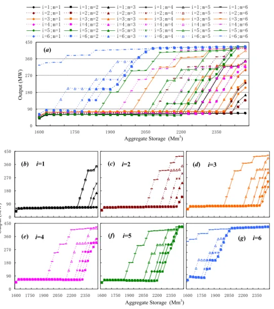
Figure 8ashows the complete operation policies derived by TS-BSDP using Strategy C for 10 days from 1 to 10 August and the operation policies of different inflow forecasts of SF froms51 tos56 are shown in Fig-ures 8b–8g. The variablessandmin Figure 8 represent inflow forecast of SF (1–5 days) and MF (6–10 days) respectively.

Figures 8b–8g represent the operation policies for one single inflow forecast interval of SF from 1 to 6, respectively. In each figure, there are six different policy scenarios due to different inflows of MF. The 10 day operation policies are obtained by weighting the operation policies of SF and MF based on the inflow intervals ofsandm. The operation policies of SF are determined byfSF

t ðÞ, in which inflow forecast (m) is

used to forecast the inflow interval (reflecting inflow trend during MF approximately) and the expected value of remaining time steps are affected bymthrough the posterior flow transition probability. The oper-ation policies of MF are determined byfMF

t ðÞ, in which the inflow forecast (s) is used to reduce the

uncer-tainty ofm.

While in AD-SDP and AD-BSDP, the 10 day inflow forecast at the current time step is only represented by a representative value of interval. Thus the variation of inflows is not reflected in the operation policies. For example, assuming that the 10 day inflow forecast is 500 m3/s, it belongs to interval 3 in AD-BSDP. Dividing the 10 days inflow into SF and MF, there are several possible combinations such as SF5300 m3/s (s52) and MF5700 m3/s (m54) or SF5700 m3/s (s54) and MF5300 m3/s (m52). These two combinations have differ-ent operation policies under the same water storage as shown in Figures 8c and 8e, respectively.

Similar to Figure 8a, Figure 9a shows the complete operation policies derived by TS-BSDP using Strategy B for 5 days from 1 to 5 August. The operation policies of the inflow forecast interval of SF froms51 tos56 are shown in Figures 9b–9g respectively.

The operation policies in Figures 8a and 9a have different meanings in terms of decision horizon. In real-time operation, the operation policies in Figure 8a represent the 10 days operation decision in future according to the scenarios ofsandm. The operation policies in Figure 9a determine the first 5 days opera-tion using the inflow forecasts ofsandm. The operation policies in Figure 9a are more effective in terms of hydropower generation, and are able to adapt to varying conditions for the next 5 days’ operation decision by updating the inflow forecasts ofsandm.

In Figures 9b–9g, the aggregate outputs, in the case of the same inflow forecasts of SF, fluctuate with vary-ing inflow forecasts of SM. Because in the recursive equationfSF

t ðÞ, the operation policies during SF are

affected by the inflow forecastssandm. The inflow forecasts (m) only affect the expected value of remain-ing time steps through the posterior flow transition probability.

While in Figures 8b–8g, the operation policies are obtained by weighting the operation policies of SF and MF based on the inflow forecast intervals (sandm). The operation policies during SF are affected not only by the expected value of remaining time steps but also by the operation policies of MF based on the weight ofsand m. Comparing with 5 day policies derived from AF-SDP, AD-SDP, and AD-BSDP, the policies in Figure 9a can make the best use of the forecast information to improve the efficiency and reliability as discussed below.

4.2. Performance Evaluation With Observed Data

The Annual Hydropower Generation and reliability are chosen as metrics to compare the performance of the operation policies derived from AF-SDP, AD-SDP, AD-BSDP, and TS-BSDP. Annual Hydropower Genera-tion is an important indicator of the hydropower system in terms of use of water resources. System reliabil-ity is defined as the probabilreliabil-ity that the system output is not lower than the minimum demand, i.e., the required firm output in this study [Hashimoto et al. 1982]. Note that reliability measures the frequency of failures only and in some cases the magnitude of failures needs to be considered particularly when the defi-cit situations for hydropower generation become severe [Raje and Mujumdar, 2010].

The performance metrics were calculated using the observed inflows from 2001 to 2010, which implies that forecast inflows are assumed to be known perfectly at the time of operation. It is expected that the results can reveal the maximum efficiency and reliability that could be achieved based on accurate information, and also show TS-BSDP can handle the different degrees of forecast uncertainty. The performance of AF-SDP,

(a)

(b) i=1 (c) i=2 (d) i=3

(e) i=4 (f) i=5 _(g) i=6

AD-SDP, and AD-BSDP is simulated using Strategy A with two decision horizons of 5 and 10 days, while the TS-BSDP model is assessed using Strategy B with a decision horizon of 5 days and Strategy C with a decision horizon of 10 days, as shown in Figure 1.

It can be seen from Table 3 that the performance indicators from the 10 days decision horizon are better than those from 5 days using observed inflows. The results confirm that use of longer-range inflows improves system performance when the inflows are accurate (in the case of observed inflows). Comparing the results from AD-SDP and AF-SDP confirms the effectiveness of the Aggregation-Disaggregation method [Mujumdar and Nirmala2007]. With both decision horizons, the Annual Hydro-power Generation values of Huilong and Taipingshao are improved significantly with AD-SDP, resulting in a greater Annual Hydropower Generation value from the hydropower system, although Huanren’s perform-ance is reduced slightly. This is because the discharges of the three reservoirs are optimized to produce a maximum amount of water at the end of a decision horizon.

In the case study, about 70% to 80% of the annual precipitation occurs in wet seasons. Thus the indicator of Annual Hydropower Generation is mainly affected by the operation in wet seasons. The results obtained in Table 3 show that AD-BSDP performs better than AD-SDP in terms of Annual Hydropower Generation. Con-versely, the system reliability indicator is mainly affected by the operation in dry seasons due to low inflows. It can be noted that the system reliability of AD-BSDP with the 5 day decision horizon is reduced when

(a) (d) (e) (f) _(g) i=3 i=4 i=5 i=6 (b) i=1 (c) i=2

compared to the 10 day horizon. Through the analysis, the posterior flow transition probability (Pt hik) is

mainly affected by observed inflow (h) at the previous time step with a shorter decision horizon. In AD-BSDP model,his used to reduce the uncertainty of inflow forecast (i). With a shortened forecast horizon, the relationship betweenhandkis enhanced, in a sense thatkis forecasted byh, instead ofi. When the forecast horizon is 10 days, the relationship is weakened by the uncertainty in inflow forecast (i).

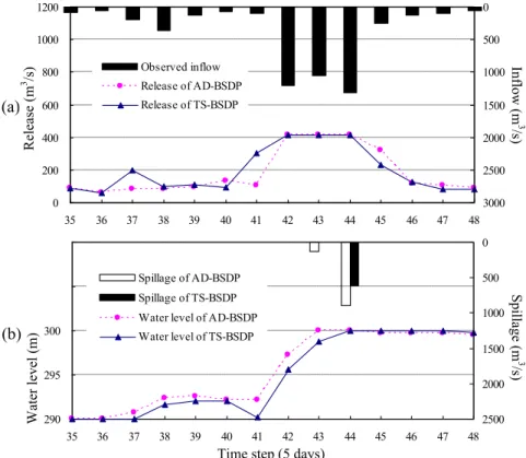
The overall performance of TS-BSDP is better than that of AD-BSDP. With the decision Strategy B, TS-BSDP uses the inflow of 10 days to determine the operation policy of the SF, while AD-BSDP uses only the inflow of SF. In order to illustrate the influence of considering the MF, the operation processes from time step 35 to 48 in the wet season of 2001 are shown as an example in Figure 10. Figure 10a shows the inflows and the releases for hydroelectric generation and Figure 10b shows the water levels and spillages of Huanren. There is a significant difference in the release at time step 41 between AD-BSDP and TS-BSDP. TS-BSDP model increases the release to reduce the storage to the dead storage volume due to the high inflow fore-casted at time step 42. Similarly, the release is reduced at time step 45 to store water for a low inflow

Table 3.System Performance From Various Optimization Models Using Observed Inflow Informationa

Models DH (days) Annual Hydropower Generation (MWH) System AHG Reliability (%) System Reliability

Huanren Huilong Taipingshao Huanren Huilong Taipingshao

AF-SDP 5 420.96 235.12 378.45 1034.53 82.36 86.53 86.67 85.19 AD-SDP 5 417.65 249.98 407.43 1075.06 84.03 87 89 93.47 AD-BSDP 5 426.86 253.56 414.15 1094.56 86.53 88.47 88.61 87.36 TS-BSDPSB 5 434.45 258.29 422.33 1115.06 85.28 92.42 84.17 94.02 AF-SDP 10 428.93 231.78 382.85 1043.56 84.44 83.83 86.39 88.89 AD-SDP 10 423.03 247.19 408.19 1078.41 85 86.44 89.17 93.61 AD-BSDP 10 429.12 252.04 418.6 1099.76 85.56 87.17 88.61 92.78 TS-BSDPSC 10 434.74 258.97 429.96 1123.68 87.5 91.17 86.67 93.05 aSB

represents Strategy B andSC

Strategy C.

forecasted at the next time step. During the operation from time step 35 to 48, the hydropower genera-tion based on the decision Strategy B of TS-BSDP is increased by 4.53 MWH compared to that from the AD-BSDP.

In Table 3, the decision Strategy C performs better than Strategy B and Strategy A of other models using observed inflows. Using observed inflows, the flow increases in wet seasons can always be identified and represented by MF. This information is used in Strategy C, as a result, the outputs of decision Strategy C are better than those of decision Strategy A. Take an example of the 10 days inflow forecast being 500 m3/s, which belongs to interval 3 in AD-BSDP. The output of AD-BSDP is 80MW with Strategy B. Dividing the 10 days inflow into SF and MF, assuming that the inflow SF and MF are in the intervalss52 andm54, the aver-age output of FH generated from Straver-agety C is 100 MW (52

63601

4

63120) using the aggregate outputs of

SF (60 MW) and MF (120 MW) with inflow intervalss52 andm54 respectively.

4.3. Performance Evaluation by Forecasts

The performance of TS-BSDP is further tested under real time operation situations. In this case, the three reservoirs are operated under the operation policies developed from various models, using the forecasted inflows from 2001 to 2010 with the QPFs. The system performances of various models are provided in Table 4.

In general, the indicator values in Table 4 are reduced compared with those in Table 3, implying that the system performance is reduced with inflow forecasts in comparison to observed data. This is due to the uncertainties in inflow forecasts. Different from the results in Table 3, the values of Annual Hydropower Generation for 5 days are better than those of 10 days. This confirms the finding that use of longer-term inflow forecasts improves system performance when the forecasts are relatively accurate (in the case of observed inflows), however the improvement is diminished as inflow forecast uncertainty increases with decision horizon extending [Simonovic and Burn, 1989;Maurer and Lettenmaier, 2003, 2004,Zhao et al., 2012].

With the decision Strategy C, TS-BSDP generates more power by 23.92 MWH than AD-BSDP using observed data as shown in Table 3. When inflow forecasts are used, however, the performance of TS-BSDP is only slightly better than that of AD-BSDP (Table 4). With a decision strategy of 10 days, the operation policies are determined by balancing the inflow information of SF and MF. The inflow forecasts over 10 days are of high uncertainty (NSE50.77), especially the inflow forecasts of MF (NSE50.56). When the decision horizon increases to 10 days, the system performance is reduced.

With the decision Strategy B, the decision horizon is 5 days. The uncertainty of MF is incorporated in deci-sion Strategy B through the posterior flow transition probabilities. While the operation policies of Strategy C are affected by not only the posterior flow transition probabilities, but also the operation policies of MF. Thus the uncertainty of MF affects the performance of Strategy C during SF more than that of Strategy B. In real-time operation, the decision horizon of Strategy B is rolled forward by 5 days, even if inflow forecasts at MF have a low accuracy, the decision Strategy B can correct the next operation decision by updating fore-cast information. The simulation results in Table 4 demonstrate that the decision Strategy B of TS-BSDP per-forms better than the others.

Table 4.System Performance From Various Optimization Models Using Inflow Forecastsa

Models DH (days) Annual Hydropower Generation (MWH) System AHG Reliability (%) System Reliability

Huanren Huilong Taipingshao Huanren Huilong Taipingshao

AF-SDP 5 414.92 233.2 375.5 1023.62 80.42 85.14 84.72 83.47 AD-SDP 5 407.61 249.92 404.6 1062.14 82 86 85 93.05 AD-BSDP 5 421.52 252.51 411.7 1085.73 85.14 87.08 87.5 85.97 TS-BSDPSB 5 421.06 258.07 416.95 1096.08 85.28 89.61 88.72 93.75 AF-SDP 10 411.78 229.13 372.74 1013.65 81.94 82.17 81.94 86.67 AD-SDP 10 404.07 240.33 401.69 1046.09 79.17 85.61 84.21 92.25 AD-BSDP 10 419.58 248.87 413.79 1082.24 83.33 87.17 87.78 92.77 TS-BSDPSC 10 419.75 254.15 414.37 1088.26 83.89 89.46 86.94 92.25 aSB

represents Strategy B andSC

4.4. Performance With Different Decision Horizons

The impact of different decision horizons on the performance of TS-BSDP is evaluated under different strat-egies. Under Strategy B, decision horizons arranging from 1 to 5 days are used to evaluate the system per-formance using both forecasted and observed data. Under Strategy C, decision horizons from 2 to 10 days are used. Figure 11 shows the Annual Hydropower Generation and reliability of TS-BSDP compared to those from BSDP under Strategy A.

With an increase in decision horizon from 1 to 5 days, the performance in Annual Hydropower Generation is generally reduced as shown in Figure 11a. Autocorrelation is used to represent a relation between the inflow in 1 day and the inflows in the preceding days. It is relatively strong in the first 5 days in the case study and can be sufficiently addressed using Markov process; thus considering a longer decision horizon (up to 5 days) does not provide valuable information for operation. However, it can be seen that the per-formance in Annual Hydropower Generation can be maintained or even improved when the decision hori-zon is greater than 5 days. This is due to the use of the flow forecasts from a longer horihori-zon which reduces unnecessary spillage. Different from Annual Hydropower Generation, the results show that the reliability increases with a longer horizon from 1 to 10 days.

The above analyses confirm the previous finding that increasing FH may generate more hydropower; how-ever, the benefits gained from a longer horizon may be offset by increasing forecast uncertainty [You and Cai, 2008;Zhao et al., 2012]. The results also reveal that it is more beneficial for system reliability to increase the inflow forecast horizon in comparison to hydropower generation. The above findings are supported with the results from all the models including TS-BSDP, which confirms the good agreement of TS-BSDP with previous models. Under both Strategies B and C, however, TS-BSDP outperforms BSDP at every horizon in terms of Annual Hydropower Generation whenever forecasted or observed data are used (Figures 11a and 11c). Similarly TS-BSDP generally outperforms BSDP in terms of reliability. It is expected that similar results could be obtained from other hydropower systems but TS-BSDP should be further tested on more complex hydropower systems and longer forecast (decision) horizons.

a _b

c d

5. Conclusions

This paper investigates the use of QPFs to improve the overall system performance of cascaded hydro-power systems in terms of hydrohydro-power generation and reliability. A new two-stage Bayesian model has been developed to quantify the uncertainties of inflow forecasts, which are considered as increasing with extending lead time, and two operation strategies have been developed to address the impact of the vary-ing magnitudes of uncertainty. The newly developed TS-BSDP is tested on the Hun River cascade hydro-power reservoirs system in China and is compared with three Stochastic Dynamic Programming models. Specifically, the findings obtained are summarized below.

1. The TS-BSDP model can effectively utilize inflow forecasts of varying uncertainty to improve system per-formance compared to three previously developed stochastic dynamic programming methods. Its com-putational efficiency is significantly improved using the virtual equivalent reservoir approach, although dividing the forecast into two periods (SF and MF) in TS-BSDP increases the complexity of the optimiza-tion problem by one dimension (which has the same dimensional complexity as AD-BSDP).

2. Splitting the forecast horizon into two periods in which inflow uncertainties are handled differently in response to the varying magnitudes of inflow forecast uncertainty is demonstrated to be an effective means of using the forecast information while addressing the uncertainty. The decision strategies based on the inflow forecast information can substantially influence the system performance. In particular, for the TS-BSDP model, the decision Strategy C performs better with observed inflows, and the decision Strategy B performs better with forecasted inflows. Further, the performance of decision Strategy C is strongly affected by inflow forecast uncertainty, and a shorter decision horizon is proven to be more effective in improving hydropower generation under this strategy.

3. This study shows that the benefit regarding hydropower generation gained from a longer horizon of inflow forecasts is diminished but the benefit reduction can be substantially mitigated through the explicit consideration of varying magnitudes of forecast uncertainties in the decision-making process. It also reveals that it is more beneficial for system reliability to increase the inflow forecast horizon in com-parison to hydropower generation.

Overall, the newly developed two-stage Bayesian model is shown to have a clear advantage in quantifying the uncertainties of inflow forecasts to improve the overall system performance of cascaded hydropower systems. It should be noted that due to the availability of QPF forecasts the performance of the new model discussed above is calculated using the 10 year QPF data, which is used to derive the operational rules. Thus, its performance should be further tested on more hydropower systems with different system charac-teristics and different sets of QPF data. In particular, the assumption that inflow forecast in SF is accurate will be further investigated with different case studies and QPFs from different numerical weather predic-tion models; although it has little impact on the performance metrics in the case study according to some preliminary investigates. In the meantime, this model addresses only the uncertainty in inflow forecasts; hence, the impacts of other uncertainty sources such as QPFs and models need to be investigated in the future work.

References

Archibald, T. W., K. I. M. McKinnon, and L. C. Thomas (1997), An aggregate stochastic dynamic programming model of multiple reservoir systems,Water Resour. Res.,33, 333–340, doi:10.1029/96WR02859.

Archibald, T. W., K. I. M. McKinnon, and L. C. Thomas (2006), Modeling the operation of multi-reservoir systems using decomposition and stochastic dynamic programming,Nav. Res. Logistics,53(3), 217–225, doi:10.1002/nav.20134.

Bartholmes, J., and E. Todini (2005), Coupling meteorological and hydrological models for flood forecasting,Hydrol. Earth Syst. Sci.,9(4), 333–346.

Bravo, J. M., A. R. Paz, W. Collischonn, C. B. Uvo, O. C. Pedrollo, and S. C. Chou (2009), Incorporating forecasts of rainfall in two hydrologic models used for medium-range streamflow forecasting,J. Hydrol. Eng.,14(5), 435–445, doi:10.1061/(ASCE)HE.1943-5584.0000014. Chang, Y. T., L. C. Chang, and F. J. Chang (2005), Intelligent control for modeling of real-time reservoir operation, part II: Artificial neural

net-work with operating rule curves,Hydrol. Processes,19(7), 1431–1444, doi:10.1002/hyp.5582.

Cheng, C. T., M. Y. Zhao, K. W. Chau, and X. Y. Wu (2006), Using genetic algorithm and TOPSIS for Xinanjiang model calibration with a single procedure,J. Hydrol.,316, 129–140, doi:10.1016/j.jhydrol.2005.04.022.

Chu, J., H. Zhou, and P. Zhang (2010), Usability analysis of classified forecast information for medium-term precipitation [in Chinese],Water Resour. Power,28(2), 4–6.

Collischonn, W., R. Haas, I. Andreolli, and C. Tucci (2005), Forecasting River Uruguay flow using rainfall forecasts from a regional weather-prediction model,J. Hydrol.,305, 87–98, doi:10.1016/j.jhydrol.2004.08.028.

Acknowledgments

This research was supported by the National Natural Science Foundation of China grants 51320105010 and 51279021, and the Hun River cascade hydropower reservoirs development company, Ltd. Fu was partially supported by the UK Royal Academy of Engineering under the Research Exchanges with China and India Scheme. Rain forecast data are downloaded from www.t7online.com.

Collischonn, W., C. E. Tucci, R. T. Clarke, S. C. Chou, L. G. Guilhon, M. Cataldi, and D. Allasia (2007), Medium-range reservoir inflow predic-tions based on quantitative precipitation forecasts,J. Hydrol.,344, 112–122, doi:10.1016/j.jhydrol.2007.06.025.

Cui, B., Z. Toth, Y. J. Zhu, and D. C. Hou (2011), Bias correction for global ensemble forecast,Weather Forecasting,27, 396–410, doi:10.1175/ WAF-D-11-00011.1.

Dutta, B., and S. J. Burges (1984), Short-term, single, multiple purpose reservoir operation: Importance of loss function and forecast errors, Water Resour. Res.,20, 1167–1176, doi:10.1029/WR020i009p01167.

Dutta, B., and M. H. Houck (1984), A stochastic optimization model for real-time operation of reservoirs using uncertain forecasts,Water Resour. Res.,20, 1039–1046, doi:10.1029/WR020i008p01039.

Fan, Y., and H. van den Dool (2011), Bias correction and forecast skill of NCEP GFS ensemble week-1 and week-2 precipitation, 2-m surface air temperature, and soil moisture forecasts,Weather Forecasting,26, 355–370, doi:10.1175/WAF-D-10-05028.1.

Hall, W. A., and J. A. Dracup (1970),Water Resources Systems Engineering, McGraw-Hill, N. Y.

Hashimoto, T., J. R. Stedinger, and D. P. Loucks (1982), Reliability, resiliency and vulnerability criteria for water resources system perform-ance evaluation,Water Resour. Res.,18, 14–20, doi:10.1029/WR018i001p00014.

Hsu, N. S., and C. C. Wei (2007), A multipurpose reservoir real-time operation model for flood control during typhoon invasion,J. Hydrol., 336, 282–293, doi:10.1016/j.jhydrol.2007.01.001.

Karamouz, M. (1990), Bayesian decision theory and fuzzy sets theory in systems operation, paper presented at the 17th Annual Water Resources Conference on Optimizing the Resources for Water Management, Am. Soc. of Civ. Eng., N. Y.

Karamouz, M., and H. V. Vasiliadis (1992), Bayesian stochastic optimization of reservoir operation using uncertain forecasts,Water Resour. Res.,28, 1221–1232, doi:10.1029/92WR00103.

Kim, Y. O., and R. N. Palmer (1997), Value of seasonal flow forecasts in bayesian stochastic programming,J. Water Resour. Plann. Manage., 123(6), 327–335, doi:10.1061/(ASCE)0733-9496(1997)123:6(327).

Liang, G. H., S. F. Xi, and B. D. Wang (2009), Ten-day Correlation Forecast Model of rainfall and runoff based on BP neural network [in Chi-nese],Water Power,35(8), 10–12.

Liu, P., S. Guo, X. Xu, and J. Chen (2011), Derivation of aggregation-based joint operating rule curves for cascade hydropower reservoirs, Water Resour. Manage.,25, 3177–3200, doi:10.1007/s11269-011-9851-9.

Liu, X. Y., S. L. Guo, P. Liu, and F. Q. Guo (2009), Study on the optimal operating rules for cascade hydropower stations based on output allo-cation model,J. Hydroelectric Eng.,28(3), 27–31 [in Chinese].

Loucks, D. P., J. R. Stedinger, and D. H. Haith (1981),Water Resources Systems Planning and Analysis, Prentice Hall, Eaglewood Cliffs, N. J. Mascaro, G., E. Vivoni, and R. Deidda (2010), Implications of ensemble quantitative precipitation forecast errors on distributed streamflow

forecasting,J. Hydrometeorol.,11(1), 69–86, doi:10.1175/2009JHM 1144.1.

Maurer, E. P., and D. P. Lettenmaier (2003), Predictability of seasonal runoff in the Mississippi River basin,J. Geophys. Res.,108(D16), 8607, doi:10.1029/2002JD002555.

Maurer, E. P., and D. P. Lettenmaier (2004), Potential effects of long-lead hydrologic predictability on Missouri River main-stem reservoirs,J. Clim.,17(1), 174–186.

McCuen, R. H. (1998),Hydrologic Analysis and Design, 2nd ed., Prentice-Hall, Englewood Cliffs, N. J.

Meneguzzo, F., M. Pasqui, G. Menduni, G. Messeri, B. Gozzini, D. Grifoni, M. Rossi, and G. Maracchi (2004), Sensitivity of meteorological high-resolution numerical simulations of the biggest floods occurred over the Arno river basin, Italy, in the 20th century,J. Hydrol.,288, 37–56, doi:10.1016/j.jhydrol.2003.11.032.

Mujumdar, P. P., and B. Nirmala (2007), A Bayesian stochastic optimization model for a multi-reservoir hydropower system,Water Resour. Manage.,21, 1465–1485, doi:10.1007/s11269-006-9094-3.

Niewiadomska-Szynkiewicz, E., K. Malinowski, and A. Karbowski (1996), Predictive methods for real-time control of flood operation of a multireservoir system: Methodology and comparative study,Water Resour. Res.,32, 2885–2895, doi:10.1029/96WR01443.

Nijssem, B., D. P. Lettenmaier, X. Liang, S. W. Wetzel, and E. F. Wood (1997), Streamflow simulation for continental-scale river basins,Water Resour. Res.,33, 711–724, doi:10.1029/96WR03517.

Ngo, L. L., H. Madsen, and D. Rosbjerg (2007), Simulation and optimization modelling approach for operation of the Hoa Binh reservoir, Vietnam,J. Hydrol.,336, 269–281, doi:10.1016/j.jhydrol.2007.01.003.

Ponnambalam, C., and B. Adams (1996), Stochastic optimization of multi-reservoir systems using a heuristic algorithm: Case study from India,Water Resour. Res.,32(3), 733–741, doi:10.1029/95WR03484.

Raje, D., and Mujumdar, P. P (2010), Reservoir performance under uncertainty in hydrologic impacts of climate change,Adv. Water Resour., 33, 312–326, doi:10.1016/j.advwatres.2009.12.008.

Roulin, E., and S. Vannitsem (2005), Skill of medium-range hydrological ensemble predictions,J. Hydrometeorol.,6, 729–744, doi:10.1175/ JHM436.1.

Saad, M., A. Turgeon, P. Bigras, and R. Duquette (1994), Learning-disaggregation technique for the operation of long-term hydroelectric power system,Water Resour. Res.,30, 3195–3202, doi:10.1029/94WR01731.

Saavedra Valeriano, O. C., T. Koike, K. Yang, T. Graf, X. Li, L. Wang, and X. Han (2010a), Decision support for dam release during floods using a distributed biosphere hydrological model driven by quantitative precipitation forecasts,Water Resour. Res.,46, W10544, doi:10.1029/ 2010WR009502.

Saavedra Valeriano, O. C., T. Koike, K. Yang, and D. W. Yang (2010b), Optimal dam operation during flood season using a distributed hydro-logical model and a heuristic algorithm,J. Hydrol. Eng.,15(7), 580–586, doi:10.1061/(ASCE)HE.1943-5584.0000212.

Serrat-Capdevila, A., and J. Valdes (2007), An alternative approach to the operation of multinational reservoir systems: Application to the Amistad & Falcon system (Lower Rio Grande/Rio Bravo),Water Resour. Manage.,21(4), 677–698, doi:10.1007/s11269-006-9035-1. Simonovic, S. P., and D. H. Burn (1989), An improved methodology for short-term operation of a single multipurpose reservoir,Water

Resour. Res.,25, 1–8, doi:10.1029/WR025i001p00001.

Stedinger, J. R, B. F. Sule, and D. P. Loucks (1984), Stochastic dynamic programming models for reservoir operation optimization,Water Resour. Res.,20, 1499–1505, doi:10.1029/WR020i011p01499.

Su, S. Y., and R. A. Deininger (1972), Generalization of white’s method of successive approximations to periodic Markovian processes,Oper. Res.,20(2), 318–326.

Tang, G. L., H. C. Zhou, N. Li, F. Wang, Y. Wang, and D. Jian (2010), Value of medium-range precipitation forecasts in inflow prediction and hydropower optimization,Water Resour. Manage.,24, 2721–2742. doi:10.1007/s11269-010-9576-1.

Tang, Y., P. M. Reed, K. van Werkhoven, and T. Wagener (2007), Advancing the identification and evaluation of distributed rainfall-runoff models using global sensitivity analysis,Water Resour. Res.,43, W06415, doi:10.1029/2006WR005813.