A large stellar evolution database for population synthesis studies. I. Scaled solar models and isochrones

Adriano Pietrinferni1

INAF - Osservatorio Astronomico di Teramo, Via M. Maggini, 64100 Teramo, Italy; [email protected]

Santi Cassisi2

INAF - Osservatorio Astronomico di Teramo, Via M. Maggini, 64100 Teramo, Italy; [email protected]

Maurizio Salaris

Astrophysics Research Institute, Liverpool John Moores University, Twelve Quays House, Birkenhead, CH41 1LD, UK; [email protected]

and Fiorella Castelli3

Istituto di Astrofisica Spaziale e Fisica Cosmica, CNR, Via del Fosso del Cavaliere, 00133, Roma, Italy; [email protected]

ABSTRACT

We present a large and updated stellar evolution database for low-, intermediate-and high-mass stars in a wide metallicity range, suitable for studying Galactic intermediate-and extragalactic simple and composite stellar populations using population synthesis techniques. The stellar mass range is between ∼ 0.5M and 10M with a fine mass spacing. The metallicity [Fe/H] comprises 10 values ranging from−2.27 to 0.40, with a scaled solar metal distribution. The initial He mass fraction ranges from Y=0.245, for the more metal-poor composition, up to 0.303 for the more metal-rich one, with ∆Y /∆Z ∼1.4. For each adopted chemical composition, the

1_{Dipartimento di Statistica, Universit`a di Teramo, Loc. Coste S. Agostino, 64100 Teramo, Italy} 2

Instituto de Astrof´isica de Canarias, 38200 La Laguna, Tenerife, Canary Islands, Spain

3

evolutionary models have been computed without (canonical models) and with overshooting from the Schwarzschild boundary of the convective cores during the central H-burning phase. Semiconvection is included in the treatment of core convection during the He-burning phase.

The whole set of evolutionary models can be used to compute isochrones in a wide age range, from ∼ 30 Myr to ∼ 15Gyr. Both evolutionary models and isochrones are available in several observational planes, employing updated set of bolometric corrections and color-Tef f relations computed for this project. The

number of points along the models and the resulting isochrones is selected in such a way that interpolation for intermediate metallicities not contained in the grid is straightforward; a simple quadratic interpolation produces results of sufficient accuracy for population synthesis applications.

We compare our isochrones with results from a series of widely used stellar evolution databases and perform some empirical tests for the reliability of our models. Since this work is devoted to scaled solar chemical compositions, we fo-cus our attention on the Galactic disk stellar populations, employing multicolor photometry of unevolved field main sequence stars with precise Hipparcos par-allaxes, well-studied open clusters and one eclipsing binary system with precise measurements of masses, radii and [Fe/H] of both components. We find that the predicted metallicity dependence of the location of the lower, unevolved main sequence in the Color Magnitude Diagram (CMD) appears in satisfactory agree-ment with empirical data. When comparing our models with CMDs of selected, well-studied, open clusters, once again we were able to properly match the whole observed evolutionary sequences by assuming cluster distance and reddening es-timates in satisfactory agreement with empirical evaluations of these quantities. In general, models including overshooting during the H-burning phase provide a better match to the observations, at least for ages below ∼4 Gyr. At [Fe/H] around solar and higher ages (i.e. smaller convective cores) before the onset of radiative cores, the selected efficiency of core overshooting may be too high in our as well as in various other models in the literature. Since we provide also canonical models, the reader is strongly encouraged to always compare the results from both sets in this critical age range.

Subject headings: Galaxy: disk — open clusters and associations: general —

1. Introduction

The availability of large sets of stellar evolution models spanning a wide range of stellar masses and initial chemical compositions is a necessary prerequisite for any investigation aimed at interpreting observations of Galactic and extragalactic, resolved and unresolved stellar populations.

A reliable library of stellar evolution models used to study stellar populations in various environments has to satisfy at least three main criteria: 1) the input physics has to be up to date and the treatment of physical processes has to be adequate and as much accurate as possible; 2) the set of models has to be homogeneous, in the sense that all evolutionary phases and initial chemical compositions have to be computed with the same evolutionary code and the same physical framework; 3) the models have to reproduce as many empirical constraints as possible.

The accuracy of the results obtained from methods based on stellar evolution models is strongly dependent on the reliability of the physical framework adopted in the compu-tations. In this respect, it is very interesting to notice that only about a decade ago the available stellar models were already producing models that matched reasonably well sev-eral observational constraints. However, new results from helioseismology came to show that solar models available at that time were seriously challenged by these new empirical results. This stimulated a large effort toward improving our knowledge of the physics of stellar matter, and as a consequence, in these last years, several aspects of stellar physics (e.g., radiative opacities, equation of state) have been largely improved. This process has produced a continuous improvement in solar models as well as in the whole stellar evolution field, with non-negligible variations in quantitative predictions, as in the case of the Galactic globular cluster ages (e.g. Chaboyer et al. 1995; Mazzitelli, D’Antona & Caloi 1995; Salaris, Degl’Innocenti & Weiss 1997). A detailed discussion of the effect of recent improvements in the input physics on the stellar evolution results can be found in Cassisi et al. (1998). This evidence provides a clear support for the need of a continuos improvement and update of stellar model databases.

The homogeneity of the adopted model library is also extremely important, because the use of different sets of models (computed by different authors with different input ph-syics) for different evolutionary phases and/or chemical compositions and/or mass ranges can introduce subtle inconsistencies in the interpretation of observations, and can affect the predictive power of stellar population synthesis techniques.

As for the comparison with empirical constraints, it goes without saying that this is the best way to assess the reliability of the chosen evolutionary scenario. In particular, it is very

important to compare theoretical models with empirical constraints from resolved stellar populations, such as Galactic field stars and Galactic stellar clusters. This is a fundamental step in order to be able to estimate the level of accuracy of the models, as well as for evaluating the uncertainties which could affect the population synthesis analysis based on the same models.

The need of continuously improved stellar evolution databases (in spite of the already existing large number of stellar models and isochrone sets) incorporating the latest advances in modeling the stellar physics cannot be more emphasized by the fact that existing dif-ferences among stellar model libraries translate into large uncertainties in, just to give an example, the ages of external galaxies; this is well illustrated by, e.g., the large differences obtained by Spinrad et al. (1997) and Yi et al. (2000), regarding the age (at least 3.5 Gyr vs. 1.4–1.8 Gyr, respectively) of an unresolved high-redshift galaxy (LBDS 53W091), due mainly to large differences in the colors (and spectra) predicted by the two different sets of isochrones used in the two mentioned papers. Such large differences due only to uncertainties in the modeling of stellar populations have important consequences for our interpretation of the epoch and mechanisms of galaxy formation.

Only by employing independent sets of stellar model databases one can assess the real uncertainties in the inferred parameters for resolved and unresolved stellar populations. In case of some key stellar input physics, like, i.e., boundary conditions, overshooting, atomic diffusion efficiency, mass loss, it is not yet clear what the best prescription is; to this one has to add current uncertainties on the synthetic spectra used to transform the output of theoretical stellar models into observed quantities like colors, magnitudes, line strengths. It is therefore necessary the availability of independent sets of models, computed with the best possible choices of the well established physics, and with various choices for the parameters describing the physical processes not yet well understood. It is therefore important that several sets of models are available, computed with the best possible inputs for the well established physics (e.g., equation of state, opacities), and with various choices of the parameters describing the physical processes not yet well understood (e.g., mixing, convection, mass loss).

The recent literature is rich of updates of stellar model libraries, see, e.g., Bono et al. (2000), Girardi et al. (2000), VandenBerg et al. (2000), Lejeune & Schaerer (2001), Yi et al. (2001) and Castellani et al. (2003); however not all of them cover homogeneously a large range of ages and chemical compositions. Over the years, we have published a lot of specialized papers with a series of specific goals, other than addressing the issue of population synthesis techniques. We have investigated the effects of improvements in the adopted physical inputs on stellar models (Salaris & Cassisi 1996; Brocato, Cassisi & Castellani 1998; Cassisi et al. 1998, 1999 and references therein); we have compared our

low mass isochrones with selected observational constraints from old stars (e.g., Cassisi & Salaris 1997; Salaris & Cassisi 1998; Riello et al. 2003) and obtained estimates of Galactic globular cluster ages (e.g., Salaris, Degl’Innocenti & Weiss 1997; Salaris & Weiss 1998, 1999, 2002), initial He abundance of globular cluster stars (Cassisi, Salaris & Irwin 2003; Salaris et al. 2004), pulsational properties of variable stars (De Santis & Cassisi 1999; Bono et al. 1997). This notwithstanding, we have never published an extended and homogeneous set of stellar models covering a large range of stellar masses, chemical compositions and evolutionary phases, suitable for population synthesis analysis as well as for any other kind of investigation making extensive use of stellar evolution models.

The main purpose of this work is to fill this gap, by providing an up-to-date and complete set of stellar models for both low-and intermediate mass, and high mass stars up to 10M, spanning a large metallicity regime from metal-poor star systems to super-metal-rich popula-tions. Our updated theoretical models are then coupled to a new set of color-transformation and bolometric corrections. In this paper, all theoretical results are based on a scaled solar metal distribution. The case of an α−element enhanced metal mixture will be the subject of a forthcoming paper.

The paper is organized as follows: § 2 summarizes the improvements made to our evolutionary code, while§3 deals specifically with the difficult problem of the core convection treatment. Our standard solar model is briefly discussed in § 4, and the model library is presented in § 5. Comparisons with the most used existing isochrone databases, and with selected empirical constraints are discussed in § 6, and § 7, respectively. A summary and conclusions follow in § 8.

2. The stellar evolution code and input physics

The stellar evolution code adopted in this work is the same used by Cassisi & Salaris (1997) and Salaris & Cassisi (1998), with various updates. We have added the nuclear burning of light elements as Li, B and Be, improved the numerical procedures that optimize the choice of both the number of mesh points within a model, and the evolutionary time steps, and updated the model input physics. In the following we summarize our choice of the most relevant input physics, and – in case of differences with our previous Cassisi & Salaris (1997) models – we discuss its impact on relevant model parameters.

• The radiative opacities are from the OPAL tables (Iglesias & Rogers 1996) for temper-atures larger than 104 K, whereas the opacities by Alexander & Ferguson (1994) which include the contribution from molecules and grain have been adopted for lower

tem-peratures. Both high and low temperature opacity tables assume a scaled solar heavy element distribution (Grevesse & Noels 1993). As for the electron conduction opacities we use the recent results by Potekhin et al. (1999) and Potekhin (1999, hereinafter P99). These computations cover also the physical conditions typical of degenerate He cores in Red Giant Branch stars; this avoids the extrapolation one had to perform with our previous choice of the Itoh et al. (1983, 1993, hereinafter - I93) conductive opacities since, as first shown by Catelan, de Freitas Pacheco & Horwath (1996), the I93 opac-ities did not cover the degenerate He cores in low mass stars. Before computing the whole set of evolutionary models presented in this work, we have tested the effect of the P99 opacity on the size of electron degenerate He cores at the He flash ignition: at a metallicity Z=0.002 the change of the He core mass at the He flash in a 0.8M model is equal to 6×10−4_M

, in the sense that the P99 opacities produce a less massive

He core with respect the I93, but at solar composition the trend reverses, the He core mass being≈7×10−4_M

larger when using the P99 opacity. It is clear that the effect

related to the use of the P99 data is not large. This notwithstanding we decided to update our code by using the P99 opacities, in order to avoid any extrapolation.

• We updated the energy loss rates for plasma-neutrino processes (relevant in the He degenerate cores) using the most recent and accurate results provided by Haft, Raffelt & Weiss (1994). For all other processes we still rely on the same prescriptions adopted by Cassisi & Salaris (1997). In case of a 1M star with Z=0.002, these new neutrino rates produce a He core mass at the He flash∼0.005M larger (and the corresponding

log(L/L is increased by ∼0.025) than our previous results based on the Munakata, Kohyama & Itoh (1985) rates. However, the same 1M star at solar metallicity (see

§4) shows an He core mass at the He flash decreased by 0.003 M (the corresponding

log(L/L is decreased by ∼0.015) with respect to our previous models.

• The nuclear reaction rates have been updated by using values from the NACRE database (Angulo et al. 1999), with the exception of the 12C(α, γ)16O reaction. For this reaction we employ the more accurate recent determination by Kunz et al. (2002). Electron screening is treated according to Graboske et al. (1973). We have tested the effect on the main sequence turn off luminosity when passing from our previously adopted rates (Caughlan & Fowler 1988) to the NACRE ones. We found that for a 1Mstar of solar composition the age at the turn off increases by 0.6 %, and log(L/L) at the turn off increases by∼ 3.5%.

The new 12C(α, γ)16O rate by Kunz et al. (2002) reduces the He burning evolutionary lifetimes (at a fixed He core core mass and envelope composition) by approximately 7-8 %, with respect to the results obtained with our previously adopted Caughlan et al. (1985) rate.

• The detailed Equation of State (EOS) by A. Irwin1 _{has been used. A full description}

of this EOS is still in preparation (Irwin et al. 2004) but a brief discussion of its main characteristics can be found in Cassisi, Salaris & Irwin (2003). This EOS can cover the entire stellar structure along all the main evolutionary phases of stars in a large mass range (including the full mass range spanned by our present models); the accuracy of this EOS is similar to the case of the OPAL EOS (Rogers, Swenson & Iglesias 1996) – and recently updated in the treatment of some physical inputs (Rogers & Nayfonov 2002) – that however does not allow the full coverage of the stellar models presented in this work. In fact, e.g., the new OPAL EOS has still an upper limit to the temperature of 108 K, and this prevents any evolutionary computation beyond the approach to the He burning ignition.

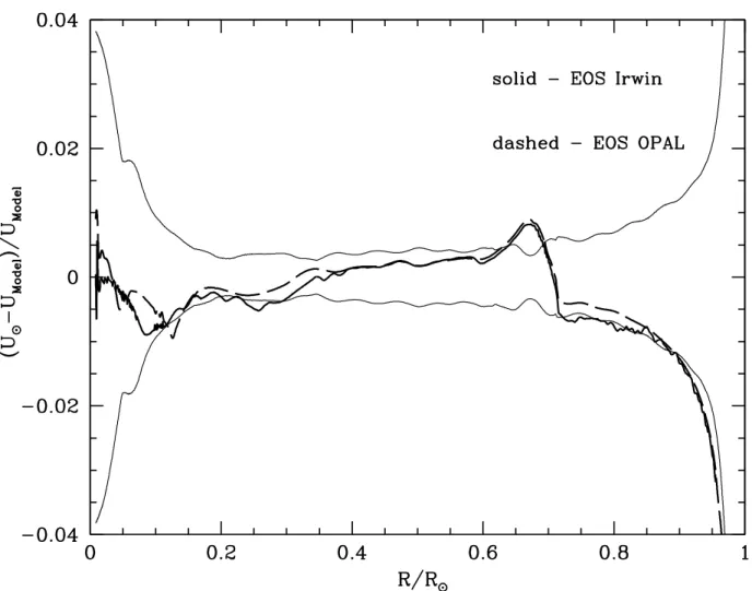
To give an idea of the differences between our adopted EOS and the OPAL one in the common range of validity, we show in Fig. 1 a comparison of the run of the ratio U=P/ρ

as a function of the distance from the star center, obtained from our calibrated solar model (see§4), and a solar model calibrated using the OPAL EOS. In both calibrated models the surface Z/X ratio, envelope He abundance and depth of the convective envelope match the empirical determinations (see below and § 4). Besides the com-parison with the values of U inferred from helioseismology (data from Degl’Innocenti et al. 1997) it is important to notice how our adopted EOS closely matches the results obtained with the OPAL one.

As for the effect of passing from the EOS used in Cassisi & Salaris (1997) to the actual one, we performed a test by computing the evolution of a 1M star of solar metallicity up to the He flash, using both EOSs and keeping everything else fixed. With the new Irwin EOS the zero age main sequence logL/L is ∼25 % brighter, and its effective temperature ∼250 K hotter; the turn off logL/L is ∼10 % brighter, its effective temperature ∼190 K higher and its age is 1.6 Gyr younger (∼16 % younger). At the He flash this age difference is preserved, whereas the He core mass is 0.01M smaller.

• Our stellar evolution code can account for the atomic diffusion of both Helium and heavy elements. The diffusion coefficients are calculated by means of a routine provided by A. Thoul (1995, private communication), which solves Burgers’s equation for a multicomponent fluid (Thoul, Bahcall & Loeb 1994, see also the in depth discussion by Schlattl & Salaris 2003). At variance with canonical computations in which the total metallicity does not change within the star, when diffusion occurs the metal abundances display a gradient across the stellar structure. However, being all elements heavier than

1

The EOS code is made publicly available at ftp://astroftp.phys.uvic.ca under the GNU General Public License (GPL)

carbon more or less equally diffused, the abundance ratios are not significantly affected by atomic diffusion, and this allows to account for the effects of diffusion on the stellar opacity simply by interpolating among scaled-solar opacity tables of different Z. We have properly accounted for atomic diffusion only when computing the standard solar models (see§4). The whole set of evolutionary models presented in this paper has been computed without including atomic diffusion. In fact, although in the Sun atomic diffusion is basically fully efficient, spectroscopic observations of, e.g., stars in Galactic globular clusters or field halo stars (see, e.g., Gratton et al. 2001; Bonifacio et al. 2002 and references therein) point to a drastically reduced efficiency of diffusion, maybe due to the counteracting effect of some sort of rotational mixing processes. This raises the possibility that the almost uninhibited efficiency of diffusion found in the Sun might not be a common occurrence. In view of this uncertainty we decided, conservatively, to not include in our model grid computation the effect of atomic diffusion.

• The outer boundary conditions have been computed integrating the atmospheric layers with theT(τ) relation provided by Krishna-Swamy (1966). Superadiabatic convection is treated according to the Cox & Giuli (1968) formalism of the mixing length the-ory (B¨ohm-Vitense 1958). The mixing length parameter has been fixed by the solar calibration and kept constant for all masses during all evolutionary phases (see, e.g., Freytag & Salaris 1999).

• All models include mass loss using the Reimers formula (Reimers 1975) with the free parameterη set to 0.4. This value of ηis commonly assumed (e.g. Girardi et al. 2000) because it allows to broadly reproduce the mean colors of horizontal branches in Galac-tic globular clusters. We are in the process of computing an additional set of models (for all metallicities in our grid) that employs η=0.2, in order to provide a tool to assess the impact of different efficiency of mass loss on various properties of simple and composite stellar populations (e.g., their integrated colors).

3. The treatment of convection at the border of convective core.

Stars with masses larger than ∼ 1.1M (the exact value depends on the initial chemical composition) during the central H-burning phase develop a convective core, due to the de-pendence of the CNO-cycle efficiency on temperature. The instability against turbulent convection is classically handled by means of the Schwarzschild criterion for a chemically ho-mogeneous fluid. This well known criterion is based on the comparison between the expected temperature gradient produced by the radiative transport of energy, and the adiabatic one. It is worth noticing that the proper estimate of the size of the convective region is then

primarily dependent on the accuracy of the input physics. Any improvement of the adopted physics may produce a change in the temperature gradients and, in turn modify the location of the boundaries of the convective regions.

A second important point concerns the possibility that the motion of the convective fluid elements is not halted at the boundary with the stable region beyond the formal convective core. Although beyond the Schwarzschild boundary a moving fluid element is subject to a strong deceleration, it might be possible that a nonzero velocity is mantained along a certain length. This mechanical overshoot may induce a significant amount of mixing in a region formally stable against convection (see Cordier et al. 2002, and references therein).

Finally, another important point which has to be taken into account is that a sizeable increase in the internal mixed region, hence larger convective cores, could be obtained as a consequence of rotationally induced mixing (Meynet & Maeder 2000).

There are therefore at least three different reasons (inadequate input physics, overshoot-ing from the convective boundary, additional mixovershoot-ing due to rotation) why the size of the ’real’ stellar convective cores might be different from the one predicted by ‘canonical’ models, that is, models computed neglecting rotation, and overshooting from the Schwarzschild convective boundary. This evidence raises the question if the size of the convective core, as determined by the (classical) Schwarzschild criterion is able to properly match the observations, or it has to be ‘artificially’ increased.

Discrepancies with observations have been usually interpreted in terms of the efficiency of anovershootingmechanism; the extension of this additional mixed region is usually defined in terms of a parameter λOV which gives the length – expressed as a fraction of the local

pressure scale height HP – crossed by the convective cells in the convectively stable region

outside the Schwarschild convective boundary.

The case for a significant amount of overshooting has been presented many times both theoretically and observationally, although in some cases the results have been contradictory (see, e.g., Testa et al. 1999; Barmina, Girardi & Chiosi 2002; Brocato et al. 2003). What is well known is the effect of including overshooting in the stellar models: during the core H-burning phase the star has a larger He core, a brighter luminosity and a longer lifetime. During the following core He-burning phase, the luminosity is brighter, the lifetime is short-er and the blue loops in the Color Magnitude Diagram (CMD) are less extended than in the absence of overshooting. Theory therefore predicts that the mass-luminosity (M-L) re-lationship for stars crossing the Cepheid instability strip is largely affected by the amount of overshooting accounted for in the stellar evolution computations. The comparison of the theoretical M-L relationship with empirical data could, in principle, put tight constraints

on the efficiency of this process. This approach has been recently adopted by Keller & Wood (2002) by adopting a large database of empirical data for Bump Cepheids and, the obtained results seem to support the occurrence of a large overshooting efficiency. Although the method is sound, the results have to be cautiously treated, as clearly shown by Cassisi (2004).

Due to the lack of a general consensus about the convective core overshooting efficiency our stellar models are computed both without overshooting and with a significant efficiency of this process. In the latter case, we adoptλOV = 0.20×HP. This value allows a good match

between to the CMD of Galactic open clusters of different ages, and allows us a comparison with the evolutionary models recently presented by other groups, all using a similar value of the overshooting parameter. The overshooting region is fully mixed as far as the chemical elements are concerned, and the temperature gradient is kept at its radiative value.

Another important issue to be addressed is the value of λOV when stars have small

convective cores. It is well known that the Turn Off (TO) morphology of the evolutionary tracks and, in turn, of the isochrones, does depend on how the extent of the convective core decreases with decreasing mass. When moving deeper and deeper inside the star, the pressure scale height steadily increases; this causes a large increase of the size of convective cores in stars whose Schwarzschild convective boundary is fast shrinking, (e.g., for masses below ≈1.5M) if the overshooting efficiency is kept fixed at a constant fraction of HP. It

is clear the need to decrease λOV to zero for stars with small convective cores, a problem

addressed theoretically by, e.g., Roxburgh (1992) and Woo & Demarque (2001).

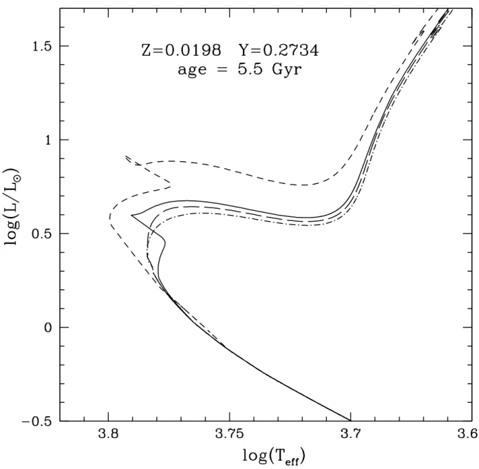
In order to show how critical this issue is, we show in Fig. 2 two isochrones of the same chemical composition and age, obtained using different assumptions about the trend of λOV

with mass. The change in the isochrone morphology is quite significant and different choices concerning the core overshoot efficiency in the critical mass range 1.0 ≥ M/M ≤ 1.52

mimic different isochrone ages. It is also worthwhile to notice the significant change in the shape of the TO region. This means that the trend ofλOV with mass, for masses with small

convective cores, potentially introduces an additional degree of freedom in stellar evolution models. Even if this problem affects only a restricted range of cluster ages, it has to be taken into account when discussing the uncertainties affecting stellar models.

In our models with core overshooting, regardless of the initial metallicity, we have chosen the following algorithm for varying the overshoot efficiency with mass: for masses larger or equal to 1.7Mwe fixedλOV at 0.20HP; for stars less massive than 1.1Mwe useλOV = 0 (we

2_{It is worth noticing that the finer details of the isochrone morphology do depend not only on the adopted}

checked that all our models of at least 1.1Mshow a central convective core during the MS), while in the intermediate range λOV varies according to the relation λOV=(M/M−0.9)/4.

We have verified by performing several numerical experiments, that this choice allows a smooth variation of the isochrone TO morphology, and a smooth decrease to zero of the convective cores for stars in this mass range.

Moreover, this choice for the overshooting extension does provide a good fit to the TO morphology of a sample of clusters of various ages, as discussed later. In particular, our overshooting isochrones fit extremely well the TO morphology of clusters like NGC 2420 and NGC 6819 where the typical TO mass is ∼ 1.3M (for [Fe/H]=−0.44) and ∼ 1.4M (for [Fe/H]=0.06), respectively, i.e. in a mass range where theλOV is decreasing according to our

prescription. The case of M 67 (Sandquist 2004, see also below) and the eclipsing binary AI Phoenicis (see below) seem however to indicate that λOV ∼0 when the stellar mass is equal

to ∼1.2M. Since we provide both overshooting and canonical models, the user can freely choose to use a criterion based on age for the switch to λOV=0 models and isochrones.

As for the convective cores during the He-burning phase, we account for semiconvection (which is driven by mechanical overshooting from the boundary of the Schwarzschild core) at the border of the canonical convective core by using the numerical scheme described by Castellani et al. (1985). Near the core Helium exhaustion we inhibited the breathing pulses (Castellani et al. 1985; Dorman & Rood 1993), following the results by Cassisi et al. (2003). The breathing pulses are suppressed adopting the procedure suggested by Caputo et al. (1989), i.e., by limiting the extent of the convective core so that the central Helium abundance cannot increase between consecutive models.

We neglect the possible occurrence of overshooting from the bottom of the convective envelopes. This choice has been made in order to reduce as much as possible the number of free parameters in the stellar computations, and also in light of the fact that there is no clear-cut empirical evidence for a sizable efficiency of this phenomenon. A critical test for this phenomenon is the comparison between the position of the RGB bump in Galactic globular clusters with the theoretical counterpart. A non negligible amount of overshooting from the bottom of the convective envelope does shift the bump to lower luminosities. This kind of test does not provide a definitive answer (e.g. Riello et al. 2003), mainly because of the uncertainty on the metallicity scale of globular clusters (the bump position is also strongly affected by the initial stellar metallicity). It is however important to remark that convective envelope overshooting can affect the morphology of blue loops during the core He-burning phase (Alongi et al. 1991; Renzini et al. 1992; Renzini & Ritossa 1994). A detailed investigation of the dependence of blue loops on the physical assumptions adopted in stellar computations and a comparison with Cepheid data will be the subject of a forthcoming

paper.

4. The standard solar model

The calibration of the standard solar model allows one to fix the value of the mixing length, as well as the solar initial He and metal fractions. In practice, one finds the combination of initial He (Y) and metal (Z) mass fractions, and the value of the mixing length parameter that reproduce the solar radius (R = 6.960×1010cm), luminosity (L = 3.842×1033ergs s−1, Bahcall & Pinsonneault 1995) and ratio (Z/X) = 0.0245±0.005 (Grevesse & Noels 1993), at an age of t = 4.57 Gyr.

The accuracy of the theoretical solar model can be then tested by comparing the depth of the outer convective layers and the surface Y value with the values 0.710 – 0.716R

(Castellani et al. 1997), and 0.2438 and 0.2443 (Dziembowski et al. 1995), respectively, as obtained from helioseismological studies.

It is well known (see, e.g., Bahcall & Pinsonneault 1992, 1995; Basu et al. 1996; Bahcall, Pinsonneault & Basu 2001 and references therein) that solar models without microscopic diffusion cannot properly account for some features of the seismic Sun. For this reason, we decided to account for atomic diffusion of both Helium and metals when computing solar models, as described in section 2.

We have computed several models with mass equal to 1M starting from the pre-MS phase, under different assumptions about the initial He and metal abundances, and mixing length parameter. The ‘best’ solar model which fulfills the quoted requirements has been obtained for an initial Y=0.2734, an initial Z = 0.0198, and a mixing length value equal to 1.913. This standard solar model is in agreement with the results from helioseismology concerning the depth of the convective envelope (0.716R) and the present surface He abundance (Y = 0.244), and with the actual (Z/X) ratio ((Z/X)=0.0244). The value of the mixing length obtained from the calibration of the solar standard model is then adopted for the whole set of models presented in this work. We will show later that this choice of the mixing length coupled with the color-effective temperature transformations used in this work allows a fine match to several observational constraints. The initial solar He abundance and metallicity (Y = 0.2734−Z = 0.0198) are the values adopted when computing the so called ’solar metallicity’ model set.

5. The stellar model library

5.1. The initial chemical composition of the model grid

As already stated, this work does provide an homogeneous and self-consistent database of theoretical stellar models and isochrones, based on the scaled solar heavy element distribution by Grevesse & Noels (1993). The extension to models accounting for a suitable enhancement of α-elements will be the subject of a forthcoming paper.

In order to cover a wide range of chemical compositions, we provide models computed for 10 different metallicities, namely Z = 0.0001, 0.0003, 0.001, 0.002, 0.004, 0.008, 0.01, 0.0198, 0.03 and 0.04.

As far as the initial He-abundances are concerned, we adopt for the lowest metallicity the estimate recently provided by Cassisi et al. (2003, see also Salaris et al. 2004) based on new measurements of the R parameter in a large sample of Galactic globular clusters. They found an initial He-abundance for globular cluster stars of the order of Y = 0.245, which is in satisfactory agreement with the recent determination of the cosmological baryon density provided by WMAP observations of the power spectrum of the Cosmic Microwave Background (CMB) radiation (Spergel et al. 2003). It is worth noticing that the theoretical

R parameter calibration used by Cassisi et al. (2003) is based on a small set of low mass

α-enhanced stellar models computed with exactly the same code and input physics of the models presented here. In order to reproduce our initial Y (see previous section) we adopt

dY /dZ ∼1.4.

In Table 1 we summarize the initial chemical composition of our model grid, and provide also the corresponding [Fe/H] value (determined assuming the observed solar (Z/X) ratio by Grevesse & Noels 1993), a quantity directly comparable to spectroscopic observations. It is important to notice that the ’solar metallicity’ models provide [Fe/H]=0.06, instead of 0. The reason is that the model grid does not include diffusion (which we know is active in the Sun, but, as discussed before, possibly inhibited at least at the surface of other low mass stars); when diffusion is included the ’solar metallicity’ composition would provide [Fe/H]=0 only at the solar age for solar-like models. This also means that our model and isochrone grid computed with the solar initial chemical composition will be unable to match the properties of the Sun, e.g., the helioseismologically determined depth of the convective envelope and the envelope He abundance, the surface Z/X ratio and in general the inner sound speed profile. This is common to all databases computed without diffusion, but on the other hand our same solar isochrones are able to fit – as we will show later – the main sequence (and the rest of the observed CMD) of the open cluster M 67, whose stars display a well established solar photospheric [Fe/H], has an age close to the solar value, and its reddening and distance

are well determined empirically.

5.2. The evolutionary tracks and isochrones

For each chemical composition, we have computed the evolution of up to 41 different stellar masses. The minimum mass is around 0.50M (slightly varying with metallicity), whilst the maximum one is always equal to 10M. In the near future we will extend the computations to both Very Low Mass stars3 and more massive stars.

In order to increase the accuracy of the numerical interpolations among different evolu-tionary tracks, needed for computing isochrones and for population synthesis studies, and to allow a detailed analysis of specific evolutionary properties, such as the Red Giant Branch transition (Sweigart, Greggio, & Renzini 1990), we adopted a mass step of 0.1M (or lower) for masses below 2.5M, 0.2M for masses in the range 2.5≤M/M ≤3.0, and 0.5M for more massive models4_.

Models less massive than ∼3M have been computed starting from the pre-MS phase, whereas the more massive ones have been computed starting from a chemically homogeneous configuration on the MS. All models, apart from the less massive ones whose central H-burning evolutionary times are longer than the Hubble time, have been evolved until the C ignition or after the first few thermal pulses along the Asymptotic Giant Branch (AGB) phase. We plan in the near future to extend the evolution of low- and intermediate-mass stars up to the end of the thermal pulses along the AGB, using the synthetic AGB technique (see, e.g., Marigo, Bressan, & Chiosi 1996 and reference therein).

In case of models undergoing a violent He flash at the RGB tip, we do not perform a detailed numerical computation of this phase; instead, we consider the evolutionary values of both the He core mass (McHe), and the surface He abundance (HeS) at the RGB tip, and

accrete the envelope with the evolutionary chemical composition until the appropriate total mass is obtained. After waiting for the thermal relaxation of the structure, the resulting Zero Age Horizontal Branch (ZAHB) model has the same luminosity of the corresponding model evolved through the He flash, as demonstrated by Vandenberg et al. (2000).

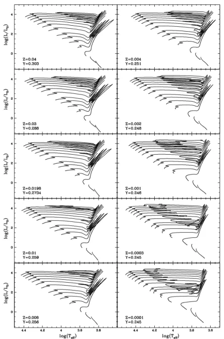
A subsample of the evolutionary tracks (canonical models) is shown in Fig. 3 for all our adopted chemical compositions. It is evident that all relevant evolutionary phases are

3_{This work will be done in collaboration with A.W. Irvin and D. Vandenberg.}

properly sampled by the different tracks.

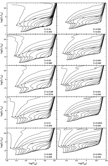
For each chemical composition we have computed additional He burning models (that is, HB models in addition to the ones obtained with our chosen mass loss law) with various different values of the total stellar mass after the RGB phase, using a fixed core mass and envelope chemical profile, as given by a RGB progenitor having an age (at the RGB tip) of ∼ 13Gyr (see Fig. 4). These models allow one to compute the CMD of synthetic HB populations, where there is a spread in the amount of mass lost along the RGB phase (like the case of Galactic globular clusters).

The RGB progenitor of these additional HB models has a mass typically equal to 0.8M

at the lowest metallicities, and increasing up to 1.0Mfor the more metal-rich compositions. For these additional computations we have adopted a very fine mass spacing, i.e. more than 30 HB models have been computed for each chemical composition. A subset of these models in displayed in Fig. 4. The very fine mass spacing provides a suitable tool for investigating the pulsational properties of RR Lyrae stars and Pop.II Cepheids as a function of the cluster metallicity and HB morphology.

All our post-ZAHB computations have been extended either to the onset of thermal pulses for more massive models, or until the luminosity along the cooling sequence of white dwarfs decreases down to log(L/L)∼ −2.5, for less massive models. They allow a detailed investigation of the various evolutionary paths following the exhaustion of the central He burning, i.e.: i) Extremely Hot Horizontal Branch stars that do not reach the AGB and evolve as AGB-manqu´e stars; ii) Post Early AGB stars, which leave the AGB before the onset of thermal pulses, and iii)bona fide AGB stars, i.e. stars massive enough to experience the AGB thermal pulses.

In order to produce isochrones for a given initial chemical composition, the individual evolutionary tracks have been reduced to the same number of points, according to a well established procedure (see, e.g., Prather 1976; Bergbusch & Vandenberg 1992). Along each evolutionary track some characteristic homologous points (key points – KPs) corresponding to well-defined evolutionary phases have been identified. The choice and number of KPs had to fulfill two conditions: 1) all main evolutionary phases have to be properly accounted for; 2) the number of KPs has to be large enough to allow a suitable sampling of the track morphology, even for faster evolutionary phases. The second condition requires also that the number of points between two consecutive KPs has to be properly chosen.

As it is well known, when passing from stars with a radiative core during the central H-burning phase to more massive stars with convective cores, the track morphology changes significantly. Therefore the KPs in this phase are different for stars with radiative or

convec-tive cores. The adopted KPs and the number of points between consecuconvec-tive KPs are listed in Table 2, whilst in Fig. 5 we show the location of the key points along a typical intermediate mass star and a low-mass He burning structure. This choice allows an adequate sampling of the track morphology for the whole evolutionary database and it guarantees accurate interpolations when using this database in population synthesis codes.

Since we have exactly the same KPs at all metallicities and the same number of points distributed between consecutive KPs, all isochrones at any age and metallicity will have the same number of points distributed consistently between corresponding evolutionary phases. This allows one to easily produce isochrones of intermediate metallicities by simply inter-polating on a point-by-point basis among the available isochrones. In this way the use of our database in a stellar population synthesis algorithm is straightforward and simple. To this purpose, we have performed a numerical test as follows. Isochrones for various ages and

Z=0.008 ([Fe/H]= −0.35) have been computed by interpolating (on a point by point basis) quadratically among the chemical compositions corresponding to Z=0.004 ([Fe/H]=−0.66),

Z=0.01 ([Fe/H]=−0.25) and Z=0.0198 ([Fe/H]=0.06). These isochrones have been com-pared to the actual isochrones of the same metallicity (Z=0.008, i.e. [Fe/H]=−0.35), com-puted from the appropriate evolutionary tracks. We found that a simple quadratic interpo-lation scheme is sufficient to reproduce the evolving masses to within a few thousandth of solar masses, colors and magnitudes within 0.02 mag or better along most of the evolution-ary phases spanned by the isochrones, log(L/L) and log(Tef f) within a few thousandth dex

along the isochrones.

The whole set of evolutionary computations (but the additional HB models discussed above) have been used to compute isochrones for a large age range, namely, from 40 Myr up to 12.5 Gyr (older isochrones can also be computed), from the Zero Age Main Sequence up to the first thermal pulse on the AGB or to the C ignition. The entire library of evolutionary tracks and isochrones are available upon request to one of the authors or can be retrieved at the URL site http://www.te.astro.it/BASTI/index.php. In the near future, we will make available at this URL site a WEB interface which will allow to any user to compute isochrones, evolutionary tracks and synthetic Color-Magnitude diagram (see below) for any specified age, stellar mass, star formation history and so on (Cordier et al. 2004).

Detailed tables displaying the relevant evolutionary features for all computed tracks are also available by ftp and at the WEB page5. We display in Tables 3 and 4 a summary of the basic information about the [Fe/H]=0.06 canonical models in selected evolutionary phases;

5

Those interested in obtaining more information, specific evolutionary results as well as additional set of models can contact directly one of the authors or use the ‘request form’ available at the quoted WEB site.

tables like these ones, for all metallicities and both canonical and overshooting models, are available at the mentioned WEB address.

The files containing the isochrones provide at each point (2000 points in total) the initial value of the evolving mass and the actual one (in principle different, due to the effect of mass loss), log(L/L), log(Tef f), MV, (U −B), (B −V), (V −I), (V −R), (V −J), (V −K),

(V −L), (H−K), on the Johnson-Cousins system. The transformation from log(L/L) and log(Tef f) to magnitudes and colors have been performed adopting a new set of bolometric

corrections and color - Tef f transformations specifically computed for this work (see the

following section for more details).

These isochrones can be used as input data for the fortran codeSY N T HET IC M AN(ager), that we have written in order to compute synthetic CMDs, integrated colors and integrated magnitudes of a generic stellar population with an arbitrarily chosen Star Formation Rate (SFR) and Age Metallicity Relation (AMR). The program reads a grid of isochrones for ages between log(t)=7.6 and 10.10 (age t in years), in steps of 0.05 dex, and a file specifying a SFR and AMR. For each time step set by the ages of the input isochrones, the program deter-mines from the SFR and AMR the number of stars formed at that age, and their metallicity. Once these quantities are computed, the program selects values for the masses of the stars formed, according to a prescribed Initial Mass Function (IMF), and interpolates among the isochrones in the grid (linear interpolation in mass, quadratic interpolation in metallicity) in order to determine the photometric properties for these objects.

The program can also account for a spread in the AMR, photometric errors, depth effects, reddening, unresolved binaries. In Fig. 6 we show an example of CMD for a synthetic population produced by this program. The simulation contains ∼90000 stars, for a Star Formation Hystory typical of the solar neighborhood (Rocha-Pinto et al. 2000a,b), using a Salpeter initial mass function, a 1σ photometric error of 0.03 mag and a 20% fraction of unresolved binaries (the mass of the secondary stars in these systems is determined following Woo et al. 2003) 6.

5.3. Color transformations and bolometric corrections

The U BV RIJ HKL synthetic photometry was computed with passbands, zero-points, and bolometric corrections as described in Castelli ((1998)), Castelli ((1999)), and Bessell,

Castel-6

In the near future, any user will be enable to run this program for generating synthetic CMDs by using a WEB interface at our URL site.

li & Plez ((1998)). Updated grids of ATLAS9 model atmospheres and fluxes (Castelli & Kurucz (2002)) were used to generate synthetic colors and bolometric corrections needed to transform from the theoretical to the observational planes.

5.3.1. The model atmospheres

New grids of ATLAS9 model atmospheres were computed for solar and several scaled solar metallicities. For this paper we used grids with metallicities [M/H] equal to +0.5, +0.2, 0.0, −0.5, −1.0, −1.5, −2.0, and −2.57. For all the models the microturbulent velocity is

ξ=2 km s−1_{. The new grids, called ODFNEW, differ from the previous ones quoted as K95}

and C97 in Castelli ((1999)) in that:

• The number of models is 476 in all the grids. They range from 3500 K to 50000 K in

Teff and from 0.0 to 5.0 in log g;

• All the models have the same number of 72 plane parallel layers from logτRoss=−6.875

to +2.00 at steps of ∆logτRoss=0.125;

• All the models are computed with the updated solar abundances from Grevesse & Sauval ((1998))8 _{and therefore with updated opacity distribution functions (ODFs),}

which now include also H2O lines;

• All the models are computed with the convection option switched on and with the overshooting option switched off. Mixing-length convection with l/HP=1.25 is assumed

for all the models. The convective flux decreases with increasing Teff and it naturally

becomes negligible for Teff of the order of 9000 K;

• The quasi-molecular absorption H-H+ _{was added to the opacity. It affects the}

ultravi-olet flux of metal-poor A-type stars (Castelli & Cacciari, 2001).

The largest differences between these models and the previous ones occur for Teff≤ 4500 K

mostly owing to the addition of the H2O contribution to the line opacity.

7

[M/H] denotes the difference in log(Z/H) with respect to the solar value; for a scaled solar metal distri-bution [M/H]=[Fe/H].

8

This metal distribution is slightly different from the one adopted for the stellar evolution computation; however the difference between the two distributions is small and does not cause any appreciable inconsis-tency.

5.3.2. The colors

The U passband is from Buser ((1978)), while theB and V passbands are from Azusienis & Straiˇzys ((1969)). The R and I Cousins colors have passbands from Bessell ((1990)). The

J KL colors were computed with passbands from Johnson ((1965)) reported also by Lamla ((1982)). For the H color the passband from Bessell & Brett ((1988)) was adopted.

Zero-points for theV magnitude and for (U−B),(B−V),(V−I),(V−R),(V −J),(V− K),(V −L) color indices were set by normalizing the computed colors for Vega to the ob-served colors. The Vega model atmosphere is from Castelli & Kurucz ((1994)) (Teff=9550 K,

log g=3.95, [M/H]=−0.5, ξ=2.0 km s−1); the Vega observed V magnitude and colors are

V=0.03, (U−B)=0.0, (B−V)=0.0 (Johnson et al. (1996)), (V−I)=−0.005, (V−R)=−0.009 (Bessell, 1983), (V −J)=0.0, (V −K)=0.0, (V −L)=0.0. For (H−K) the computed index of Sirius was normalized to the observed one (H−K)=−0.009 (Glass 1997). The Sirius model is from Kurucz (1997) (Teff=9850 K, log g=4.30, [M/H]=+0.4,ξ=0.0 km s−1, He/H=+0.5).

After some preliminary comparisons with open cluster MS loci, we have decided to use only for MS stars with Teff≤4750 K, and only for (B−V), (V −I) and (V −R) colors, the

empirical color-Teffrelationships provided by Houdashelt, Bell & Sweigart (2000).

The bolometric correction BCV is given by:

BCV =−2.5[log(σTef f4 /π)−log( Z β

α

SV(λ)F(λ)dλ)] +K

where SV(λ) is the V passband and F(λ) is the computed flux. The constant K was defined

by normalizing to zero the smallest bolometric correction (in absolute value) of the whole synthetic grid computed for [M/H]=0.0 and microturbulent velocityξ=2.0 km s−1_{. It occurs}

for the model withTeff= 7250 K, log g=0.5. With this normalization, positive values for BCV

are avoided. The value of BCV is −0.203 for a solar model with parameters Teff=5777 K,

log g=4.4377,ξ=1.0 km s−1_.

By assuming V=−26.75 (Hayes,1985), the solar absolute magnitude is MV=4.82.

Therefore, for the adopted normalization, Mbol is given by MV+BCV=4.62.

All the ODFNEW grids of models and colors are available at the URL sites

http://kurucz.harvard.edu/grids.html and http://wwwuser.oat.ts.astro.it/castelli/grids.html. In Fig. 7 we display a comparison of our 500 Myr (including overshooting) and 10 Gyr [Fe/H]=0.06 isochrones, transformed to the MV −(V −I) CMD by using our adopted

trans-formations discussed before, plus the Yale (Green 1988), NEXTGEN (Allard et al. 1997) and older ATLAS 9 (Castelli 1999) ones. This comparison is representative of the general

differences in the various color planes covered by our isochrones. The Yale transformations tend to produce a bluer lower MS, RGB and He-burning phase, whereas the cooler and brighter part of the RGB tends to agree with our results. Color differences can be as high as ∼0.2 mag. The NEXTGEN transformations are available for surface gravities higher or equal to log(g)=3.5 (in cgs units), and are different (bluer) only on the lower MS. The earlier ATLAS 9 transformations are very similar apart from the lower MS and cooler RGB, where color differences of∼0.2 mag or more are reached.

6. Comparison with existing databases

In this section we compare the H-R diagram of selected isochrones with the counterparts from the publicly available databases by Girardi et al. (2000), Castellani et al. (2003), Lejeune & Schaerer (2001) and Yi et al. (2001). In addition, we add a comparison with Bergsbusch & Vandenberg (2001) isochrones kindly provided by the authors (D.A. VandenBerg 2003, private communication).

These various grids of models are computed employing some different choices of the physical inputs (opacities are usually the same, but EOS, nuclear reaction rates, boundary conditions and neutrino energy loss rates are often different), and also the chemical compo-sitions are generally different. We perform the comparison on the theoretical H-R diagram, thus bypassing the additional degree of freedom introduced by the choice of the colour trans-formations. We employed our isochrones including overshooting (unless otherwise stated), since all these sets of isochrones are computed including overshooting from the convective cores, albeit often with different prescriptions about its extension and the decrease to zero for decreasing stellar mass.

We have selected isochrone ages that span all the relevant age range, and chemical compositions as close as possible to our choices. It is important to notice that Castellani et al. (2003) and Yi et al. (2001) models do include atomic diffusion (He and metals for Castellani et al. models, only He for Yi et al. models), and therefore their isochrones for old ages (above a few Gyr) are affected by the efficiency of this process.

Figure 8 shows a comparison with the Girardi et al. (2000) isochrones; the chemical composition of our isochrones is as labeled, very close to theZ=0.019,Y=0.273 composition of Girardi et al. (2000) isochrones. The selected ages are 100 Myr, 500 Myr, 1.8 Gyr and 10 Gyr, respectively. The MS loci do agree reasonably well, whereas our RGBs are sys-tematically hotter, apart from the youngest isochrone. Our He-burning models are slightly brighter, especially for the 500 Myr isochrone, but become fainter at 100 Myr. The TO

regions are in good agreement at 10 Gyr; our TO models become brighter at 1.8 Gyr, have the same luminosity as Girardi et al. (2000) but are hotter at 500 Myr, and are fainter at 100 Myr. At 1.8 Gyr the TO region of Girardi et al. (2000) isochrones is reproduced if we select an age higher by 0.7 Gyr (e.g., the mass evolving at the TO of our isochrone is higher than the Girardi et al. 2000 counterpart); at 100 Myr we need to choose an age 10 Myr younger to reproduce the TO of Girardi et al. (2000) isochrones. Since Girardi et al. (2000) computed also a set of canonical isochrones for this metallicity, we have investigated in more detail the reason for the relatively large difference at 1.8 Gyr. We discovered that the differ-ence between the 1.8 Gyr old canonical isochrones – which are only due to the differdiffer-ence in the model input physics – accounts for about 40% of the discrepancy between the overshoot-ing models. The remainovershoot-ing fraction of the discrepancy has to be ascribed to the interplay between the overshooting treatment and the different input physics.

In Fig. 9 we display a comparison with selected isochrones without overshooting and initialZ=0.008 andY=0.250, from the database by Castellani et al. (2003). The agreement with our canonical models is quite good all along the MS, TO region and RGB. Our He-burning luminosities are slightly lower, and at 10 Gyr there is a larger difference at the TO region due to the effect of atomic diffusion included by Castellani et al. (2003). We do not find a substantial discrepancy in the TO brightness at 1.8 Gyr, as in case of the comparison with the canonical models by Girardi et al. (2000).

The comparison with Lejeune & Schaerer (2001) models with initial Z=0.004 and

Y=0.252 is displayed in Fig. 10. Ages are the same as in the previous comparison. The isochrone MSs of the two sets look in reasonable agreement, and the TO region of the oldest and youngest isochrones are practically identical. However for the 500 Myr and 1.8 Gyr the TO of our isochrones is clearly brighter. At 1.8 Gyr we should employ an isochrone about 1 Gyr older in order to match the Lejeune & Schaerer (2001) one. Our RGBs are much hotter and the He-burning phase (when available in Lejeune & Schaerer 2001 isochrones) is brighter at 500 Myr and fainter at 100 Myr.

In case of the Yi et al. (2001) database, we compared with the Z=0.02, Y=0.27 isochrones, for ages of 100 Myr, 600 Myr, 1.8 Gyr and 10 Gyr (see Fig. 11). Also in this case the MS loci appear to be in good agreement, apart from the lower luminosities, where Yi et al. (2001) models show a different slope. The TO of their 10 Gyr isochrone is affected by diffusion, and behaves accordingly when compared with our models. At 100 and 500 Myr the brightness of the TO regions is similar, although effective temperatures are slightly dif-ferent; at 1.8 Gyr there is again a difference in the TO luminosity, that translates into an age difference of about 800 Myr, as in case of the comparison with Girardi et al. (2000) isochrones; our RGBs are hotter at all ages.

The comparison with VandenBerg isochrones (Y=0.277 and Z=0.0188) is shown in Fig. 12, for ages of 2 and 10 Gyr. The 10 Gyr isochrones do agree very well also along the RGB. At 2 Gyr we find the same differences encountered in the other comparisons.

A common result of the previous discussion is the fact that our RGB temperatures are generally hotter than the others, and the TO luminosity for our 1.8 Gyr isochrones is higher. As far as the RGB temperatures are concerned, the difference is certainly not due (apart from the comparison with Vandenberg models, where the RGB location is exactly the same in the 10 Gyr isochrones which have the same RGB evolving mass, and with Castellani et al. models) to different value of the mass evolving along the RGB (higher masses when our isochrones are brighter at a given age), since we find this difference also with respect to isochrones with the same RGB evolving mass. We will see in the next section that this difference in the RGB temperatures – possibly due to a combination of different EOS, and solar mixing length calibration obtained using different boundary conditions, see e.g. Salaris, Cassisi & Weiss (2002) – does not prevent our models from fitting very well the observed RGBs in a sample of Galactic open clusters, when coupled to our color transformations. To justify better why we think these effective temperature discrepancies along the RGB may be due to a combination of different boundary conditions and EOS, we notice that in Salaris, Cassisi & Weiss (2002) it has been shown how different boundary conditions (for example grey vs Krishna SwamyT(τ) relationship) produce different solar mixing length calibrations that make all solar models agree at the Sun location, but disagree along the RGB by differences of the order of 100 K. As for the influence of the EOS, the same 1M solar composition models discussed in §2, computed using the Irwin EOS and the EOS employed in Cassisi & Salaris (1997) keeping everything else unchanged, show Tef f differences along the RGB of

the order of ∼ 280 K at the base of the RGB, ∼140 K at log(L/L)=2 and ∼85 K at the He flash ignition, in the sense of having hotter temperatures with the Irwin EOS.

As for the TO brightness differences at 1.8 Gyr (which however is negligible in case of the comparison with Castellani et al. 2003 models without overshooting), it persists for ages higher than 1.8 Gyr, up to when the overshooting distance and the size of the convective cores are reduced to zero (ages of about 5–6 Gyr). We believe that this might be related mainly to the different MS lifetime caused by the use of a different EOS, coupled to differences in the way the overshooting distance is reduced to zero when approaching the radiative core regime.

To conclude this section, we show in Fig. 13 a comparison between our ZAHB luminosity at the instability strip vs [Fe/H] theoretical relationship, and analogous results from various authors. Our new values are systematically brighter than Cassisi & Salaris (1997) models, due mainly to the effect of the new plasma neutrino rates and the higher initial He content

(in Cassisi & Salaris 1997 we employed a primordial He mass fraction equal to 0.23). The main difference in Cassisi et al. (1998) models is the EOS for the electron degenerate cores along the RGB, that increases the He flash core mass with respect to our result (they also used the I93 electron conduction opacities that slightly increase the He core mass in this metallicity range), but this increase is offset by the fact that their adopted He abundance is lower. Vandenberg et al. (2000) models are the faintest ones of this group, and we believe this is mainly due to their use of the Hubbard & Lampe (1969) electron conduction opacities (that produce a lower He core mass at the He flash with respect to our adopted opacities), coupled to a lower primordial He abundance. The results by Caloi et al. (1997) have an overall different slope with respect to the other models, and we are not able to exactly pinpoint the reason for this difference.

7. Empirical tests

In this section we present the results of some empirical test we performed in order to es-tablish the consistency of our models with photometric constraints. We have successfully tested our models in Cassisi et al (2003) and Riello et al. (2003), in the regime of Galactic globular clusters. In particular, we have shown that with our models the initial He abun-dance of globular clusters as estimated from the R-parameter, is finally in agreement with the cosmological constraint (Cassisi et al. 2003). More tests on Galactic globular cluster stars (whose initial chemical composition is characterized by [α/Fe]>0) will be presented in the companion paper with theα-enhanced model grid. The reason for this is twofold. First, scaled solar isochrones are not an appropriate surrogate for α-enhanced ones with the same

Z when Z is above ≈0.002 (e.g. Salaris & Weiss 1998); second, from our new α-enhanced color transformations we have found that. e.g., scaled solar (B −V)-effective temperature relationships are different from α-enhanced ones, starting from relatively low metallicities around Z ∼ 0.001.

In the comparisons detailed below, we employed the CMDs of field stars and a sample of clusters with empirically established parameters like distance, [Fe/H] (and scaled solar metal mixture) and reddening. In this way we do not have much freedom to change the parameters of our models in order to match the observations. Comparisons with, e.g., LMC clusters would be much less meaningful, since reddenings, [Fe/H] (especially) and distances (not only the distance to the LMC barycenter, but also geometrical effects) are not well established empirically. We could fit the CMDs of those clusters and give our estimates of their distance and reddening by playing with combinations of reddening, distance and [Fe/H], but this would not be a real test for the accuracy of the models.

We also refrained from comparing theoretical integrated colors with galactic open clus-ters or LMC data. The problem is that integrated colors of galactic open clusclus-ters are very uncertain due to their low total mass that induces large stochastic color fluctuations pre-venting any meaningful comparisons (see, e.g., the numerical experiments by Bruzual & Charlot 2003 and the integrated colors reported in the WEBDA database – Mermilliod 1992 – at http://obswww.unige.ch/webda/integre.html). The same applies to LMC clusters, with the additional problems of not well known age and uncertain reddening. The situation is better for the more massive Galactic globular clusters, and in fact we will perform (using the appropriate α-enhanced theoretical isochrones and color transformations) this comparison in our forthcoming paper about α-enhanced models.

In the following comparisons, when necessary, we will use the reddening law AV =

3.24E(B−V),AI = 1.96E(B−V), andAK = 0.11AV (Schlegel, Finkbeiner & Davis 1998).

7.1. Solar neighborhood MS stars

Percival et al. (2002) have published homogeneous multicolor photometry and photo-metric metallicity estimates for a large sample of local field dwarfs with accurate Hipparcos

parallaxes; the [Fe/H] values of the individual stars range from ∼ −0.4 up to +0.3. These data are extraordinarily well suited to test the MS location of our theoretical isochrones in various colour bands; moreover, the choice of the isochrone age is irrelevant, since the observed stars are all unevolved, i.e. fainter than MV ∼5.5.

We have divided the Percival et al. (2002) sample into three subsamples, as follows. The most metal poor subsample comprises objects with [Fe/H] between−0.35 and−0.15, with an average value of [Fe/H]=−0.24±0.06; the intermediate subsample contains stars with [Fe/H] between−0.05 and +0.15, with an average value of 0.06±0.06. The third subsample is made of the most metal rich objects, with [Fe/H] between 0.16 and 0.36, and an average [Fe/H] equal to 0.26±0.09. In Figs. 14 to 18 we compare the CMD of these three subgroups with our isochrones for [Fe/H]=−0.25, 0.06 and +0.26, respectively. The comparison is made in theMV −(B−V),MV −(V −I),MV −(V−R) andMK−(V −K),MK−(J−K) planes; the

J andK magnitudes of the field stars come from the 2M ASS database (M. Groenewegen & S. Percival, private communication), and have been transformed to our adopted IR system following Carpenter (2001). For the sake of comparison we also show a Girardi et al (2000) isochrone with [Fe/H]=0.06.

The agreement between the empirical CMDs and the isochrones appears to be satis-factory – in the sense that the theoretical isochrones usually overlap the main CMD locus

occupied by the dwarfs in the various metallicity bins and color planes– although it tends to deteriorate slightly – apart from the case of MK −(V −K) – at the highest metallicity

(where, however, the star sample is the smallest).

7.2. Open clusters

We have employed a sample of galactic open clusters of various ages for further tests of the reliability of the magnitudes and colors of our isochrones. More in detail, we have con-sidered the CMDs of the Hyades (Pinsonneault et al. 2003), NGC 2420 (Anthony-Twarog et al. 1990), M 67 (Sandquist 2004) and NGC 188 (BV from Caputo et al. 1990, andV I from von Hippel & Sarajedini 1998), for which precise parallax-based distance determinations do exist. In case of the Hyades accurate parallaxes of the individual stars in the observed CMD have been determined by the Hipparcossatellite. For the other clusters the distances have been determined by Percival & Salaris (2003 – PS03) using a completely empirical MS-fitting method presented in Percival et al. (2002). The MS template sequences used in this technique have been computed making use of the field dwarf sample by Percival et al. (2002), whose individual [Fe/H] values are on the same scale of the open cluster metallic-ities by Gratton (2000). PS03 employed clusters’ [Fe/H] estimates from Gratton (2000) and reddening from Twarog et al. (1997).

When we compare our models to the observed CMD of a cluster, we have chosen within our isochrones grid the one with metallicity closest to the cluster [Fe/H]. However, if no com-puted isochrone has a [Fe/H] value within the quoted 1σ error associated to the cluster one, we interpolate quadratically within our grid as previously discussed, in order to determine the isochrone with the precise cluster metallicity.

We will consider a fit ’successful’ when the theoretical isochrones overlap the main cluster CMD branches for values of reddening, metallicity and distance modulus in agreement with the empirical determinations.

Figures 19 and 20 display the comparison with the Hyades CMD corrected for the cluster distance; the cluster metallicity is [Fe/H]=0.13 according to Gratton (2000), and the reddening is zero. The observed CMD contains exactly the same stars in all three different photometric planes. The interpolated isochrone with [Fe/H]=0.13 that best matches the Hyades CMD has an age of 790 Myr if overshooting is included, or 560 Myr for canonical models; notice the match (that in (B −V) and (V −K) degrades only when MV >7.5) of

the unevolved MS to the observed one, without applying any colour shift. The TO region inK−(V −K) is however less well reproduced with respect to the BV I CMD, a fact that

can be ascribed either to some inconsistencies in the color transformations, or photometric data or a combination of both.

In case of NGC 2420, PS03 obtained (m−M)0 = 11.94±0.07, assuming [Fe/H]=−0.44

and E(B−V) = 0.05±0.02; our interpolated isochrones with [Fe/H]=−0.44 that best match the observed CMD provide a distance modulus (m−M)0 = 11.90 and E(B −V)=0.06, in

good agreement with the MS-fitting results (see Fig. 21). The age of the best fitting isochron with overshooting is 3.2 Gyr, whereas the canonical one has an age of 2 Gyr. It is interesting to notice that the isochrone with overshooting does provide a better match of the observed CMD TO region.

As for M 67, PS03 have determined a distance modulus (m−M)0=9.60±0.09, adopting

E(B−V)=0.04±0.02 and [Fe/H]=0.02±0.06. Their MS-fitting determination was based on a differentBV I photometry (Montgomery et al. 1993), however Sandquist (2004) has obtained exactly the same distance modulus with his photometry, employing the same method by PS03 and the same [Fe/H] and E(B −V). We fitted our [Fe/H]=0.06 isochrones to the

BV I cluster data, and obtained a successful fit with E(B−V)=0.02 and (m−M)0=9.66, in

agreement, within the error bar, with the MS-fitting results. The result of the fit is shown in Fig. 22. The MS and RGB of the cluster appear to be matched by both overshooting and canonical isochrones; also the brightness of the He-burning stars is reproduced. It is also worth noticing that Sandquist (2004, his Fig. 14) has shown how a number of isochrones in the literature is unable to fit the main location of the MS for V > 15.5−16, when the empirical distance, reddening and metallicity are considered; our isochrones, however, do provide a much better match to this MS region. The ages of the best fitting isochrones are 4.8 Gyr and 3.8 Gyr for the overshooting and canonical models, respectively. As already noticed by Sandquist (2004) who employed the Yi et al. (2001) and the Girardi et al. (2000) isochrones, the overshooting models do provide a worse fit to the TO region compared to the canonical ones. The mass evolving at the TO of the overshooting isochrone is equal to

∼