Title Statistical Inference in Markov Switching Vector ErrorCorrection Model Using a Markov Chain Monte Carlo Method
Author(s) Sugita, Katsuhiro
Citation 琉球大学経済研究=Ryukyu University EconomicReview(92): 37-63
Issue Date 2016-09-30
URL http://hdl.handle.net/20.500.12000/36147
Statistical Inference in Markov Switching Vector
Error Correction Model Using a Markov Chain
Monte Carlo Method
Katsuhiro Sugita*
Faculty of Law and Letters, University of the Ryukyus, Nishihara,
Senbaru, Okinawa, 903-0213, Japan
E-Mail: [email protected]
Abstract
This paper introduces statistical inference in a Markov switching vec-tor error correction model using a Markov chain Monte Carlo method. The proposed model allows for regime shifts in the deterministic terms, the lag terms, the adjustment terms and the variance-covariance matrix. The pro-posed method allows for estimation of the cointegrating vector within a non-linear framework through a collapsed Gibbs sampling. We apply the pro-posed model to U.S. term structure of interest rates.
Key words: Bayesian inference; Nonlinear cointegration; Markov switching model; Gibbs sampling; Bayes factor;
*The author would like to thank Mike Clements and the participants of seminar at Warwick, Hitotsubashi, and Kobe University for their useful comments.
1 Introduction
This paper proposes a Markov switching vector error correction model (MS-VECM) that allows for regime shifts in the deterministic terms, the lag terms, the adjust-ment terms and the variance-covariance matrix in a vector error correction model, using a Bayesian approach with a Markov chain Monte Carlo method.
A number of studies consider nonlinear cointegration models with regime switch-ing. Balke and Fomby (1997) consider a threshold cointegration model to inves-tigate the model in which there is discontinuous adjustment to a long-run equi-librium, based on the idea that only when the deviation from the equilibrium ex-ceeds a critical threshold, do the benefits of adjustment exceed the costs and, hence economic agents act to move the system back toward the equilibrium. Ander-son (1997), Tsay (1998), Martens et al (1998), and Clements and Galvao (2002) are examples of applying threshold cointegration model. Krolzig (1997) develops a regime switching cointegration model using Hamilton's (1989) Markov regime switching process instead of threshold cointegration model. Hall et al ( 1997) ana-lyze the permanent income hypothesis using a single equation cointegration model with Markov regime switching. Psaradakis et al (2004) employ Markov switching to analyze an error correction model in a single equation. A vector error correction model with Markov regime switching is applied by Sarno and Valente (2005) for forecasting stock returns, and by Clarida et al (2006), who show regime switching in the term structure of interest rates.
Estimation for the MS-VECM by classical methods requires a multi-stage max-imum likelihood procedure. The first stage consists of testing for the number of cointegrating relationships in the system and estimating the cointegrating vectors by implementing Johansen's (1988, 1991) maximum likelihood method. The sec-ond stage consists of estimating other parameters in the model by maximum likeli-hood method. Thus, the cointegrating vectors and other parameters in a nonlinear
-Statistical Inference in Markov Switching Vector Error Correction Model Using a Markov Chain Monte Carlo Method (~EB )Jj~)
vector error correction model are estimated assuming the model is linear. The final stage consists of the implementation of an expectation-maximization (EM) algo-rithm for maximum likelihood estimation for unobserved Markov state variables conditional on estimated values of the cointegrating vectors and other parameters by maximum likelihood. Thus, to estimate the Markov state variables, the maxi-mum likelihood estimates are treated as if they were the true values.
By applying a Bayesian approach, estimation of the MS-VECM is more ef-ficient as inference on the state variable is based on a joint distribution, rather than a conditional distribution. The cointegrating vectors are estimated based on a joint distribution of other variables including the state variables, so that it allows estimation of the cointegrating vectors within a nonlinear framework, rather than assuming that the model is linear.
This paper proposes a Bayesian approach to the MS-VECM that allows any set of the parameters in the model to shift with Markov process. For a Bayesian approach to the MS-VECM, Paap and van Dijk (2003) propose a nonlinear VECM where only intercept terms are affected by Markov regime shift to investigate U.S. consumption and income. They employ a Bayesian approach based on Kleibergen and Paap (2002), which requires linear normalizing restrictions on the cointegrat-ing vectors. This linear normalizcointegrat-ing restrictions is criticized by Strachan (2003) as being likely to be invalid. Strachan and van Dijk (2003) and Strachan and lnder (2004) discuss the further problems associated with the use of linear normaliz-ing restrictions, and propose the Grassman approach that places a valid prior on the cointegrating space. See Koop, Strachan and van Dijk (2006) for details. In this paper, we apply the method by Koop, Leon-Gonzalez and Strachan (forth-coming) who develop further prior elicitation for the cointegrating space. They propose an efficient posterior simulation algorithm for cointegrated models using a collapsed Gibbs sampler. Examples of application of this method include Koop,
Leon-Gonzalez, and Strachan (2006) for a cointegrating panel data model and Stra-chan and van Dijk (2007) for model averaging in vector autoregressive models.
Our model in this paper is more general than Paap and van Dijk (2003), and is flexible to modify to consider the model in which other parameters are also subject to the regime shift. For example, in this paper we assume that the cointegrating vectors are unaffected by the regime shifts. It is, however, possible to consider the model where the cointegrating vectors are also dependent on the regime shifts. Also, it is possible to consider the trend or the drift in the cointegration relations to be affected by the regime shifts by a slight modification.
The plan of the paper is as follows. Section 2 presents estimation method for the MS-VECM using a collapsed Gibbs sampler. We specify prior densities and likelihood functions, and then derive the posterior distributions. Section 3 il-lustrates application to U.S. term structure of interest rates using the MS-VECM. Section 4 contains concluding remarks. All results reported in this paper are gen-erated using Ox version 5.10 (see Doomik, 2007).
2 Markov Switching Vector Error Correction Model
This section introduces the MS-VECM and presents a Bayesian approach to es-timate this model. Let y1 denote an /(1) vector of 1 x n with r linearcointe-grating relations. A VAR system with normally distributed Gaussian innovations
£1 rv iidN(O, Q) can be written as a vector error correction model (VECM) with the
number of lags p
p
llyt =Yr-tf3a+8fJ+ LllYr-lrt+er (1)
l=l
where a ( r x n) is adjustment term; {3 ( n x r) is cointegrating vector;
r
1 ( n x n)is lag term. The deterministic terms 8 fJ ( 8 is 1 x d, and fJ is d x n) are defined as
-Statistical Inference in Markov Switching Vector Error Correction Model Using a Markov Chain Monte Carlo Method <~m MJ~)
follows. For example, if the process contains both a constant and linear time trend, then 8
=
(J.l',
i)'
ando
= (
1 ,t), or if the process contains a constant but no time trend, then 8=
J.l and 5=
1. If we assume that the deterministic term 8, the adjust-ment terma,
the lag termsr
1, and the variance-covariance matrix .Q in the VECM are subject to an unobservable discrete state variable s1 that evolves according toa m-state, first-order Markov switching process with the transition probabilities,
p(s, = i
I
s1-t = j) = q;b i,j = 1, ...,m,
then the VECM representation is written asp
fly, = Yt-1Pa(s,)
+
o8(sr)+
E
flYt-lrl(s,)+
e,(s,) (2)1=1
where
e
1(s1 ) rv N(O,D.(s1 )).2.1 Likelihood
The MSVECM in (2) can be rewritten as
fly,= Z1,rPa(s,) +z2,rcl>+er(s,) (3)
where Z2,r = ( lt ( 1
)o, ... ,
t, (m)o,
t, ( 1 )L\y,_,, ... ,z, (
1 )L\Yr-p, ... , t,(m )L\Yr-1, ... , lt (m )L\Yr-p ),ci>
=
(8'(1), ... ,8'(m),r~(1), ... ,r~(l), ...,r'
1(m), ... ,r~(m))', zt,r =Yr-h andZ1 ( i) in z2,r is an indicator variable that equals to 1 if regime is i at t, and 0
oth-erwise. From (3 ), let define the T x n matrices Y
= (
fly~, ... , fly~ )' and E=
( ef(sJ), ... , e~(sr) )',theTxnmatrixZ;=( ~.
1
z0
(i),z'
1,2z1(i), ... ,
Zt,rlr-t(i) )', the T x m(d+np) matrix X= ( z~ 1, ~2
, ••• , z~T )',the T x h (where h =' ' ,
m(r+d+np))matrixW=( z
1
~, ... , Zm~, X ),thehxnmatrixB=( a'(I), ... , a'(m), <1>' )', then we can simplify the model as follows:m y [, Z;/3 a; +X <I>+ E i=l
-
WB+E
(4)
(5)The likelihood function for B,!l(l), ... ,!l(m),
J3
and the state variablesSr
=
{ St, s2, ... , sr }' is given by,i! ( B,/3,0(0), ... ,O(m),Sr
I
Y)
oc (
fi lil{j)
~-t,fZ)
exp (-~tr [~
{il{it
1(Y; - W;B )
1(Y; - W;B)}])
(
6) =(fi1n{j)l-'d
2) exp (-i
~
[(vec(Y;- W;B))1 (Q(j)0/
1.f
1
(vec(Y;-
W;B))])
(7)
(8)
where Y;
=
.F;Y, W;=
J;W, J; is a vector consists of 1 if j-th row's regime is i and 0 otherwise, and t; is the total number of observations when s1 = i, i = 1, ... , m.The likelihood function for the transition probabilities q;j, i, j = 1, ... , m, which are independent of the data set and the model's other parameters but conditional on the set of the state variables, is given:
where m;,j, i, j
=
0, ... , m, denotes the number of the transition from the regime ito j, that can be counted from given Sr. This likelihood for the transition probabilitiesis used by Albert and Chib (1993) and Kim and Nelson (1998).
-Statistical Inference in Markov Switching Vector Error Correction Model Using a Markov Chain Monte Carlo Method (~m ~~~)
2.2 Priors
In selecting a prior density for cointegrating vectors, one approach is to choose an informative prior such as a normal or a Student t distribution with
?-
linear normalization restrictions on {3 for identification such that {3' =(In {3;) where {3* is ( n - r) x r unrestricted matrix. Bauwens and Lubrano ( 1996) and Kleibergen and Paap (2002) choose this type of prior with linear normalization on {3.Recently, several authors have argued that it is important to elicit a prior on the space spanned by the cointegrating vectors rather than to a particular identified choice for these vectors (see Strachan (2003), Strachan and lnder (2004), Strachan and van Dijk (2004 and 2006), Villani (2005 and 2006), Koop, Leon-Gonzalez, and Strachan (forthcoming)). Strachan (2003) and Strachan and Inder (2004) criticize the linear normalization on the cointegrating vector restricts the estimable region of the cointegrating space. Koop et al (forthcoming) develop efficient posterior simulation algorithms using a collapsed Gibbs sampler to estimate cointegrating space. The approach we use in this paper is based on the collapsed Gibbs sampling method proposed by Koop et al (forthcoming).
They propose the following transformation.
where 1C
=
(aa')112 is positive definite matrix and a= JC-1a is semi-orthogonal.Then, we assign the multivariate normal distribution to the prior for b as
(10)
For a prior for the transition probabilities q;j, i, j = 1, ... , m, we assign a beta dis-tribution
q;; rv beta ( Uii, Uij) (11)
(12)
h b ti b d. .b . . h d . (
I
)
r(u;;+uij) uu-1 ( 1 w ere eta re ers to a eta tstn utton wtt enstty 1t p;; u;;, Uij=
r(uu)r(uij) P;; -P II .. )llij-l •With regard to priors forB, .Q(i) in (5), we assume prior independence between Band .Q(i) such that p(B,.Q(1), ... ,.U(m)) = p(B)I1~1 p(.Q(i)). We assign prior for the variance-covariance matrix as an inverted Wishart distribution with the de-grees of freedom vo(i) as
.Q{i) rv lW (.Uo(i), Vo(i)) (13)
where .Q0(i) E Rnxn_ As for a prior forB, we consider the vector form of
Bun-conditional on .Q(i) because if we consider that the prior forB is conditional on .Q{i) as is often used in regression models with the natural conjugate priors, it is not convenient to consider a case when the error covariance is subject to change with regime. We assign prior for B as a multivariate normal as
vec(B) rv MN(vec(Bo)
,r.n
0) (14)where MN refers to a multivariate normal with mean vee (Bo) E JR.nhx 1, and
variance-covariance matrix r,80 E JR.nhxnh.
2.3
Posterior SpecificationsIn this subsection we derive the posterior densities from the priors and the like-lihood functions. First, we derive the state variable S-r: = { s1 , s2 , ... , s-r: }' by the
-44-Statistical Inference in Markov Switching Vector Error Correction Model Using a Markov Chain Monte Carlo Method (~HI ~~~)
multi-move Gibbs sampler, then derive the posterior distributions for other param-eters.
To sample the state variable St we employ the multi-move Gibbs sampling method, which is originally proposed by Carter and Kohn (1994) and is applied to a Markov switching model by Kim and Nelson (1998). The multi-move Gibbs sampling refers to simulating s1, t = 1, 2, ... , T, as a block from the following
con-ditional distribution:
T-1
p
(sT
1 e,Y)=
p(st 1 e,Y) Ilp(st 1 st+l,e,Y)t=p
(15)
where 9 =
{B,Jj,.Q(1), ...
,.Q(m),qll, ... ,qmm}· The first term of the right hand side of the equation (15), p(s-r
I e,
Y), can be obtained from running the Hamil-ton filter (HamilHamil-ton, 1989). To draw s1 conditional on s1+ 1,e
and Y, we use the following results:p(s,
I
Sf+t,0,Y)
=
p(st+lI
s(,e,~~~)
I
e,Y) oc p(st+lI
s,)p(s,I
e,r)
(16)p St+I
M'
where p(sr+l
I
sr) is the transition probability, and p(s,I
e,Y) can be obtained from the Hamilton filter. Using Equation (16) we compute:p (
-OI
E>Y)- p(sr+IIsr=1)p(sr=1IE>,Y)07)
r St- St+I, ' - LJ=IP(St+I
I
St=
j)p(sr=
jI
e,Y)Once above probability is computed, we draw a random number from a uniform distribution between 0 and I, and if the generated number is less than or equal to the value calculated by (17), we set s1 = 1, otherwise, set equal to 0.
After drawing S-r by multi-move Gibbs sampling, we generate the transition probabilities, q00 and q11 , by multiplying (11) and (12) by the likelihood function (9)
Next, we can construct X and Z in (4) using the draw of S-r, and then the joint posterior distribution can be obtained from the priors given in (13) and (14) and the likelihood function forB, f3,il(i), and
S-r,
that is,p (
B,p,n(t), ... ,n(m),Sr
1Y)
oc p(B,p,n(1), ... ,n(m),Sr)
£(B,p,n(t), ... ,n(m),Sr
1Y)
oc g(b)
[D
(1ilo(i)l"'(i)/2IO(i)I-(',+Vo(i)+n+l)/2)] I EBo l-112 exp {-~
[ tr(tn(it
1)+
~
[vec(Y;- W;B)'(O(i)
®l,,t1 vec(Y;- W;B)]+
[vec(B- B0)'E;;,
1vec(B-Bo)]]}
where g (b) refers to the prior for
J3
given in ( 1 0). From the joint posterior, we have the following posterior distributions:Q(i)
I
f3,B,S-r,Y rv IW ( (Y;- W;B)' (Y;- W;B) +ilo(i),t;+
Vo(i)
+n+
1) (19)(20)
where
M*
= {
Efj~
+
t.
[!l(i)-
1 ®(W/W;)]}
-I-Statistical Inference in Markov Switching Vector Error Correction Model Using a Markov Chain Monte Carlo Method (~m IJi~)
To obtain the conditional posterior for the cointegrating vectors, we rewrite the expression in ( 4) as m
Y
-XCI> -EZ;f3a(i) +E
i=l mEZ;ba(i) +E
i=l (21) 1 1where
a(i)
andbare
such thata(i)
=
(a(i)a(i)')-1a(i)
andf3
=
b(b'b)-1.
Then vectorize both side of (21) asm
vec(Y-XCI>) -
Evec(Z;ba(i))+vec(E)
i=lm
- L
(a(i)'
®Z;)vee( b)+ vee( E)
(22) i=lor
y=Ab+e
(23)where
y
=vec(Y-
XCI>),A
=
E~1
a(i)'
® Z;,b
=
vec(b ),
ande =vee( E).
With the priorforb
rvMVN(bo, Vb
0), that is,b
rvMN(vec(bo), Vb
0), the conditional P<?Sterior
distribution of b; is obtained as
(24)
where
vb.
=[Vb;;
1+
~
{
(a(i)!l(i)-
1a(i)')
®(zfz;)}] -•
Given the conditional posterior distributions, we implement the Gibbs sam-pling to generate sample draws. The following steps can be replicated until con-vergence is achieved.
• Step I: Set j
=
I. Specify starting values for the parameters in the model, s,o)= {
s\0)'s~O)'
•••'s~O)
r
B{O)' J3 {0) andQ~O).
• Step 2: Generate n( i) (j) from p( n( i)
I
s;-
1)' {3 (j-l)' BU-1)' y) for i = 0, 1. • Step 3: Generate vec(B)U) from p( vee( B)I
s;-
1) ,f3U-I) ,n(o)Ul ,n( I )U), Y),then obtain a*(O), a* (I), and <t>j. Compute a(i)* using a(i)* = ( a(i)* a(i)*') 1/2 a(i)* fori= 0, I.
• Step 4: Generate b* from
p(b
I
w-
1)' B(j)'.Q(
0)(j) '.Q(
I) (j)' Y). Then, com-putef3/i)
=
b7(bj'bj)-~ and a(i)(j)=
a(i)*(bj'bj)~ fori= 0, 1.• Step 5: Generate the transition probabilities
(q;;)(j)
from p ( q;;I
w-•))
in (18) fori= 0, 1.• Step 6: Generate
w)
= {sP)
's~j)'
...'sV)}
I from p (S-r I
eU),y)'
where E>=
{B,.Q(O),.Q(l),f3,q
00,q
11 } in (15), using multi-move Gibbs samplingalgorithm.
• Step 7: Set j
=
j+ I, and go to Step 2.Step 2 through Step 7 can be iterated N times to obtain the posterior means or standard deviations. Note that the first No times iterations are discarded in order to
attenuate the effect of the initial values. To check the Gibbs sampler to converge to a sequence of draws from the posteriors, Geweke ( I992) suggests the MCMC diagnostic that tests whether the estimate based on the first set of the draws after No
burn-in replications is the same as the estimate based on the last set of the draws.
-Statistical Inference in Markov Switching Vector Error Correction Model Using a Markov Chain Monte Carlo Method (~IB 1151)
3 Application: U.S. Term Structure of Interest Rates
In this section, we present an empirical study using the MS-VECM to analyze U.S. term structure of interest rates.3.1 Expectation Hypothesis
The expectations hypothesis of the term structure of interest rates implies an f-period interest rate is the weighted average of the expected future one-f-period inter-est rates plus risk premium. For an overview of the expectations hypothesis theory, see Shiller ( 1990). Let r J,t be the yield to maturity for an
f
-period at time t, L J,t bethe risk premium for an /-period at timet, then the hypothesis implies:
f
rf,t
=
f-
1 [,Erri,t+i-1 +LJ,t i=I(25)
By rewriting the above equation, the interest rate spreadS J,r can be expressed as
J-I i
SJ,t
=
rf,t- rt,t=
f-
1L L
E,ilrt,t+j+
LJ,t· i=l j=l(26)
If r1 ,1 is integrated of order one, then r J,t is also integrated of order one and thus r J,t
and rt ,1 are cointegrated with cointegrating vector ( 1, -1) as analyzed by Campbell and Shiller (1987). The risk premium is assumed to be
/(0)
so that the hypothesis states that r J,r - r1 ,1 - L J,t is a stationary process.The expectations hypothesis in (26) with constant risk premium implies the following vector error correction model with the lag length at p:
p
ily, =
11
+
(Yr-tf3- LJ,r)a+
[,ilYr-lrl+
e,
(27) /=1where y1
= (
r1,1, r1,, )';a (1 x2)
is the adjustment term; f3(2
x1)
is theThere is a number of research that confirms nonlinearity of U.S. term structure of interest rates due to changes in monetary policy. Tsay ( 1998), Hansen and Seo (2002), Clements and Galvao (2002) use a threshold cointegration model, while Clarida et al (2006) employ a Markov switching vector error correction model to detect regime switching. All these studies find nonlinearity due to the instability for interest rates between 1979 and 1982 as a potential source of shifts. This period between 1979 and 1982 is known as the non-borrowed reserves operating
proce-dure, that the Federal Reserve moved from interest rate targeting to money growth
targeting and allowed the interest rate to fluctuate freely.
3.2 MS-VECM
We apply the MS-VECM to U.S. term structure of interest rate based on (27) to account for the regime shifts. The MS-VECM considered in Section 2 is applied:
p
!!y, -
Tls,
+
(Yr-tf3- Ls,)as,
+ [,
!!y,_;rL,s,
+
Er,s,
(28)l=l
p
-
Jls, +Yr-tf3as,
+
[,!!y,_;rL,s, +Er,s,
l=l(29)
where
Jls,
=Tls, - Ls, as,, £
1,s,
rvN (
0, O.s,);Ls,
is the risk premium term dependingupon the state variables.
We analyze U.S. term structure of interest rates using the MS-VECM described above. The data set is monthly Federal fund rate,
rf,
and 1-year Treasury bill rate,rf,
covering the period 1960:1 to 2008:8 with 584 observations, obtained from the Federal Reserve Bank of St. Louis. Figure 1 plots the data set and its spread.Let y1
=
(rfrf),
then we consider the following seven models:'
-Statistical Inference in Markov Switching Vector Error Correction Model Using a Markov Chain Monte Carlo Method (~III Jl~)
p
~1:
Ay, =J.l+Yr-tf3a+ EAy,_zrl+e,
I= Ip
~2:
ll.y,
=J.l(s,) +Yr-tf3a+ EAy,_zrl
+& 1=1p
~3:
Ay,
=J.l(s,)
+
Yr-tf3a(s,)
+
E
ll.y,_zrl
+
e,1=1
p
~4:
Ay, =J.l(s,)+Yr-lf3a+ Lil.Yt-lrl+e,(s,)
l=lp
~5:
Ay, =J.l(s,)+Yt-tf3a(s,)+ EAYr-Lrz+e,(s,)
I= Ip
~6:
ll.y,
=
J.l(s,)
+
Yr-lf3a
+
E
Ay,_zrz(s,)
+
e,(s,)
I= Ip
~7:
Ay,
=
J.l(s,) +Yr-tf3a(s,)
+
EAy,_lrl(s,) +e,(s,)
1=1
where
e,
r-.J iidN(O, .Q) and E1 (s1 ) r-.J iidN(O, .Q(s1 ) ). ~1 represents a linear VECM,and other models, ~2 -~7, are various specifications of the MSVECMs. To estimate these models, we implement the collapsed Gibbs sampling al-gorithm described Section 2.2, For prior hyperparameters, we set
bo
= ( 1, -1 )', Vho=.Qo(i)
=
0.01h andVo(i)
=
0.001for i=
0 or 1 in (13), Es=
100/K"nandBo
=
0 in ( 14) favoring the absence of cointegration. These values are assigned to ensure fairly large variances for representing prior ignorance. For prior hyperparameters for the transition probabilities, we setuoo
=
uu
=
9, uo1=
uw
=
1 in (11) and (12). The Gibbs sampler is run with 40,000 times with the first 5,000 discarded.In this paper, selection of the number of the rank and lags is treated as a problem of model selection. In Bayesian framework, the posterior model probability
p(
~jI
Y) is used to assess the degree of support for each model, ~j· From the Bayes rule, we have p(~jI
Y)=
p(YI
~j)P(~j)/p(Y), where p(YI
~j) is referred to as the marginal likelihood for ~j; and p(~j) is the prior model probabilityfor
.4
1. Since p(Y) is often hard to calculate, comparison of two models, Jft1 and .A;, by the posterior odds ratio, PO 1;, is often used to obtain the posterior model probability. The posterior odds ratio is defined as the ratio of their posterior d I b b'l' . PO ( JfI
Y)/ ( JfI
Y) p(YI.-ltj)p(./tj) h hmo e pro a 1 tttes as Ji
=
p Jn J p Jrt;=
p(YI.-lt;}p(A'I;) , w ere t eratio of the marginal likelihoods
~~~t~?
is defined as the Bayes factor. With the posterior odds ratios, we can obtain the posterior model probability as p(Jft1I
Y)=
PO Ji /E2!: 1
POk; where M is the number of models under consideration. Thus, inorder to obtain the posterior model probability by the posterior odds, we need to calculate the Bayes factor.
There are several methods to calculate the Bayes factor such as Chib ( 1995), Gelfand and Dey (1994), the Savage-Dickey density ratio (see Verdinelli and Wasser-man, 1995), and the Schwarz Bayesian information criterion (BIC) approxima-tion method (Schwarz, 1978). Chib ( 1995) provides a method of computing the marginal likelihood that utilizes the output of the Gibbs sampler. The marginal likelihood can be expressed from the Bayes rule as
p(y
I
.A;) = p(yI
et)P( et)p(
er
I
y) (30)where p(y
I
8j) is the likelihood for .A; evaluated at 8j, which is the Gibbs output or the posterior mean of 8;, p( 8;*) is the prior density and p( 8;*I
y) is the poste-rior density. If the exact forms of the marginal posteposte-riors are not known like our case, p( 8;*I
y) cannot be calculated. To estimate the marginal posterior density evaluated at 8;* using the conditional posteriors, first block (} into l segments as8
= (
8f, ... , 8{)', and define cp;-t= (
8f, ... , 8{_1) and cpi+ 1= (
8f+ 1, ... , 8{). Sincep( (}*
I
y)=
n~=
I p( 8;*I
y, cpj_l)' we can draweF)'
cpi+ 1 ,(j}' where j indicates the Gibbs output j=
1 ' ... 'N, from ( 8;' ... ' (}I)= (
8;' cpi+ 1 ) rv p ( 8;' cpi+ 1I
y' cpj_ 1 ) ' andthen estimate ji( 8;*
I
y, cpj_1) as-52-Statistical Inference in Markov Switching Vector Error Correction Mcxlel Using a Markov Chain Monte Carlo Methcxl (~ffi Jl~)
Thus, the posterior
p(
er
I
Y) can be estimated as(31)
Choosing a model among .-41 - .-47 and testing for cointegration rank with various lag length p = 1 to 3 is conducted using the Chib's method. There are three possible rank (r
=
0, 1, and 2) for models with lag length p=
1 to 3 where the adjustment term is constant (.-41, --42, .-44, and .-46). Thus, for models with constanta,
we consider 3 x 3 x 4=
36 models. There are two possible rank (r=
1 and 2) for models with p=
1 to 3 where the adjustment term changes according to the regime (.43, .-44, and --47,). Thus, for models with regime dependenta,
we consider 2 x 3 x 3
=
18 models. Therefore, we consider total 54 models and select the most appropriate model among them. From the results of computing the Bayes factors for all 54 models shown in Table 1, the highest posterior model probability is 47.0 percent given to a model of .-45 with p=
2 and r=
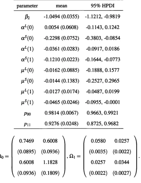
1. Table 2 reports the results of the posterior estimation of the parameters for .-45 withp
=
2 and r=
11• From the results, the 95% off3
(after normalizing) contains/32. = - 1, that is implied by the expectations hypothesis of the term structure. To examine whether the restriction of /32.
=
-1 is appropriate in a more formal way 2,we calculate the Bayes factor as BF ~ exp[-0.5(BICR-BICuR)], where BICuR is the unrestricted BIC, and BICR is the restricted BIC with the restriction of
f3
= (
1,-1), and the value is 132.52, which shows a very strong evidence to support the
1 Geweke's MCMC convergence diagnostic test (Geweke 1992) for one element of the
cointegrat-ing vector generates the statistic -0.17187 with probability 0.43177, that means a sufficiently large number of draws has been taken.
2 As Koop (2004) note, "the justification for using the HPDis to compare models is an informal
expectations hypothesis. 3
The posterior expectation of the state variables is plotted in Figure 2. The
non-borrowed reserves operating procedure between 1979 and 1982 is detected as the regime shift. Regime shift occurs also in 1973 and 1984. These regime shifts are corresponding to higher inflation regime (Goodfriend, 1998), and are characterized by a much higher variance of both the long and the short interest rate than those of regime 1. In regime 1, that is relatively stable period, the variance of the long rate is higher than that of the short rate; on the other hand, in regime 0, the short rate fluctuates much more than the long rate.
We find that the magnitudes of the adjustment terms for the short-term rate for both regimes are larger than those for the long-term rate, which implies that the short-term rate tends to adjust toward the equilibrium in either regime. The posterior mean of the adjustment term for the short rate in regime 0,
aJ,
is -0.2298, which is faster than that for the short rate in regime 1 of lower volatility. This implies that interest rates adjust much faster in periods of high volatility with high inflation and anti-inflationary monetary policy.4 Conclusion
In this paper we consider a Markov switching vector error correction model where the adjustment terms, the lag terms, the intercept terms, and the variance-covariance matrix are subject to the regime shifts with the first order unobservable Markov process while the cointegrating vector is unaffected by the regime shifts. 4
Estimations are carried out entirely by a Bayesian method. The
cointegrat-3 See Kass and Raftery ( 1995) for a rule of thumb for evaluating Bayes factors. According to this
rule of thumb, if BFij is between 20 and 150, there is a strong evidence against model j, and if BFij
exceeds 150, there is a very strong evidence against model j.
4It is possible to allow the cointegrating vectors to change with Markov process by slight modifi-cation. However, we have not done this because changing the long-run relationship is not reasonable idea unless economic theory support this.
-Statistical Inference in Markov Switching Vector Error Correction Model Using a Markov Chain Monte Carlo Method (~ffi ~~~)
ing vector is drawn using the Markov Chain Monte Carlo method by Koop, Leon-Gonzalez, and Strachan (forthcoming) in a nonlinear framework so that the estima-tion of the cointegrating vector is more efficient than multi-step classical methods where the cointegrating vector is estimated assuming the model is linear.
As an application to illustrate the use of the MS-VECM, we illustrate U.S. term structure of interest rates using the MS-VECM with regime dependent risk premium. We find that regime with high volatility and high speed of adjustment captures the non-borrowed reserves operating procedure during the 1979-82 and other phases of inflation scare, while the stable regime with low volatility and low speed of adjustment prevails after the mid of 80's.
In this paper Markov switching is chosen as a switching behavior, assuming that one regime jumps to another regime suddenly at particular dates. It is of inter-est to consider alternative multivariate nonlinear models such as a smooth transition vector error correction models (ST-VECM) to analyze the nonlinear cointegration where the regime shifts occur not suddenly but smoothly, and compare the ST-VECM with the MS-ST-VECM by the Bayes factors.
References
[1] Albert, J. H. and S. Chib (1993): "Bayes inference via Gibbs sampling of au-toregressive time series subject to Markov mean and variance shifts," Journal
of Business and Economics Statistics, 11 (1 ), 1-15.
[2] Anderson, H. M. ( 1997): "Transaction costs and non-linear adjustment to-wards equilibrium in the US treasury bill market", Oxford Bulletin of
Eco-nomics and Statistics, 59, 465-483.
[3] Balke, N. S. and T. B. Fomby (1997): "Threshold cointegration",
[ 4] Bauwens, L. and M. Lubrano ( 1996): "Identification restrictions and poste-rior densities in cointegrated Gaussian VAR systems", in T. B. Fomby (ed.),
Advances in Econometrics 11 B, Greenwich, CT: JAI press.
[5] Campbell, J. Y. and R. J. Shiller (1987): "Cointegration and tests of present value models", Journal of Political Economy, 108, 205-251.
[6] Carter, C. K. and P. Kohn (1994): "On Gibbs sampling for state space mod-els", Biometrika, 81, 541-553.
[7] Chib, S. (1995): "Marginal likelihood from the Gibbs output", Journal of the
American Statistical Association, 90, 432, Theory and Methods, 1313-1321.
[8] Clarida, R. H., L. Sarno, M. P. Taylor, and G. Valente (2006): "The role of asymmetries and regime shifts in the term structure of interest rates", Journal
of Business, 79, 1193-1224.
[9] Clements, M. P. and A. B. Galvao (2002): "Testing the expectations theory of the term structure of interest rates in threshold models", Macroeconomic
Dynamics, 1-19.
[1 0] Doornik, J.A. (2007): Object-Oriented Matrix Programming Language
Us-ing Ox, London: Timberlage Consultants Press.
[11] Gelfand, A. and D. Dey (1994): "Bayesian model choice: asymptotics and exact calculations", Journal of the Royal Statistical Society Series, B56,
501-514.
[ 12] Geweke, J. ( 1992): "Evaluating the accuracy of sampling-based approaches to the calculation of posterior moments", in Bernardo, J., J. Berger, A. Dawid, and A. Smith (eds.). Bayesian Statistics, 4, 641-649. Oxford: Clarendon
Press.
-Statistical Inference in Markov Switching Vector Error Correction Model Using a Markov Chain Monte Carlo Method <~m JB154)
[13] Goodfriend, M. (1998): "Using the term structure of interest rates for mon-etary policy", Economic Quarterly, 19, Federal Reserve Bank of Richmond, 1-23.
[14] Hall, S. G., Z. Psaradakis and M. Sola (1997): "Switching error-correction models of house prices in the United Kingdom", Economic Modelling, 14, 517-527.
[15] Hamilton, J. (1989): "A new approach to the economic analysis of nonsta-tionary time series and the business cycle", Econometrica, 51, 357-384. [16] Hansen, B. E. and B. Seo (2002): "Testing for two-regime threshold
coin-tegration in vector error-correction models", Journal of Econometrics, 110, 293-318.
[ 17] Johansen, S. ( 1988): "Statistical analysis of cointegrating vectors", Journal
of Economic Dynamics and Control, 12, 231-254.
[18] Johansen, S. (1991): "The power function for the likelihood ratio test for cointegration:, in J. Gruber, ed., Econometric Decision Models: New Methods
of Modelling and Applications, New York: Springer Verlag, 323-335.
[19] Kass, R. E. and A. E. Raftery (1995): "Bayes factors", Journal of the
Ameri-can Statistical Association, 90, 773-795.
[20] Kim, C. J. and C. R. Nelson (1998): "Business cycle turning points, a new coincident index and tests of duration dependence based on a dynamic factor model with regime switching", Review of Economics and Statistics, 188-201. [21] Kleibergen, F. and R. Paap (2002): "Priors, posteriors and Bayes factors for a Bayesian analysis of cointegration", Journal of Econometrics, 111, 223-249. [22] Koop, G. (2004): Bayesian Econometrics. Wiley.
[23] Koop, G., R. Leon-Gonzalez and R. Strachan (2006): "Bayesian inference in a cointegrating panel data model", Woking Paper, University of Leicester, UK.
[24] Koop, G., R. Leon-Gonzalez and R. Strachan (forthcoming): "Efficient pos-terior simulation for cointegrated models with priors on the cointegration space", Econometric Reviews. 29(2), 224-242
[25] Koop, G., R. Strachan and H. van Dijk (2006): "Bayesian approaches to coin-tegration", in The Palgrave Handbook of Theoretical Econometrics edited by K. Patterson and T.Mills. Palgrave Macmillan.
[26] Krolzig, H. M. (1997): Markov-Switching Vector Autoregressions. New York: Springer.
[27] Martens, M., P. Kofman and T. C. F. Vorst (1998): "A threshold error-correction model for intraday futures and index returns:, Journal of Applied
Econometrics, 13, 245-263.
[28] Paap, R., and van Dijk, H.K., (2003): "Bayes Estimates of Markov Trends in Possibly Cointegrated Series: An Application to US Consumption and In-come", Journal of Business and Economic Statistics, 21, 547-563.
[29] Psaradakis, Z., Sola, M., Spagnolo, F., (2004): "On Markov Error-Correction Models, With an Application to Stock Prices and Dividends", Journal of
Ap-plied Econometrics, 19, 69-88.
[30] Sarno, L., and G. Valente (2005): "Modelling and forecasting stock returns: Exploiting the futures market, regime shifts and international spillovers",
Journal of Applied Econometrics, 20, 345-376.
[31] Schwarz, G. (1978): "Estimating the dimension of a model", Annals of
Statis-tics, 6, 461-464.
-Statistical Inference in Markov Switching Vector Error Correction Model Using a Markov Chain Monte Carlo Method (~ffi ~~~)
[32] Shiller, R. J. (1990): "The term structure of interest rate", in Friedman, B. and F. Hahn (eds). Handbook of Monetary Economics, 1, North-Holland: Ams-terdam.
[33] Strachan, R. W. (2003): "Valid Bayesian estimation of the cointegrating error correction model", Journal of Business and Economic Statistics, 21, 185-195. [34] Strachan, R. W. and H. K. van Dijk (2003): "Bayesian model selection with an uninformative prior", Oxford Bulletin of Economics and Statistics, 65, 863-876.
[35] Strachan, R. W. and H. K. van Dijk (2004 ): "Valuing structure, model uncer-tainty and model averaging in vector autoregressive process", Econometric
Institute Report EI 2004-23. Erasmus University Rotterdam, Rotterdam.
[36] Strachan, R. W. and H. K. van Dijk (2006): "Model uncertainty and Bayesian model averaging in vector autoregressive processes", Discussion Papers in
Economics No. 06/5. Department of Economics, University of Leicester, UK.
[37] Strachan, R. W. and H. K. van Dijk (2007): "Bayesian averaging in vector autoregressive processes with an investigation of stability of the US great ratios and risk of a liquidity trap in the USA, UK and Japan", Econometric
Institute Report EI 2007-11. Erasmus University Rotterdam. Rotterdam.
[38] Strachan, R. W. and B. Inder (2004): "Bayesian analysis of the error correc-tion model", Journal of Econometrics, 123, 307-325.
[39] Sugita, K. (2009): "Bayesian Analysis of a Vector Autoregressive Model with Multiple Structural Breaks" ,Economics Bulletin, 3 (27), 1-7.
[40] Tsay, R. S. (1998): "Testing and modeling multivariate threshold models",
[ 41] Verdinelli, I. and L. Wasserman ( 1995): "Computing Bayes factors using a generalization of the Savage-Dickey density ratio", Journal of the American
Statistical Association, 90, 614-618.
[42] Villani, M. (2005): "Bayesian Reference Analysis of Cointegration",
Econo-metric Theory, 21, 326-357.
[43] Villani, M. (2006): "Bayesian Point Estimation of the Cointegration Space",
Journal of Econometrics, 134, 645-664.
-Statistical Inference in Markov Switching Vector Error Correction Model Using a Markov Chain Monte Carlo Method (~EEl JJ1~)
Table 1: Model Selection for U.S. Term Structure of Interest Rate
.411
.412
.413
.414
.415
.416
.417p=l
r=O
0.000 0.000 0.000 0.002r=l
0.000 0.000 0.003 0.012 0.152 0.011 0.032r=2
0.000 0.000 0.000 0.000 0.000 0.000 0.000p=2 r=O
0.000 0.001 0.003 0.006r=l
0.000 0.000 0.027 0.073 0.470 0.052 0.102r=2
0.000 0.000 0.000 0.000 0.004 0.000 0.003p=3 r=O
0.000 0.000 0.000 0.000r=l
0.000 0.000 0.000 0.001 0.025 0.003 0.008r=2
0.000 0.000 0.000 0.000 0.000 0.000 0.000 Note: Each value in the Table shows the posterior model probability calculated by using the Chib's method.Table 2 Posterior Results for
.415
with p = 2 ()=standard deviationparameter mean 95% HPDI
f3z -1.0494 (0.0355) -1.1212, -0.9819 aL(o) 0.0054 (0.0608) -0.1143, 0.1242 as(o) -0.2298 (0.0752) -0.3803, -0.0854 aL(t) -0.0361 (0.0283) -0.0917, 0.0186 as(l) -0.1210 (0.0223) -0.1644, -0.0773 J.LL(o) -0.0162 (0.0885) -0.1888, 0.1577 J.Ls(o) -0.0144 (0.1383) -0.2527, 0.2965 J.LL( 1) -0.0127 (0.0174) -0.0487, 0.0199 J.Ls(l) -0.0465 (0.0246) -0.0955, -0.0001 Poo 0.9814 (0.0067) 0.9663, 0.9921 Ptt 0.9276 (0.0248) 0.8725, 0.9682 0.7469 0.6008 0.0580 0.0257 Oo= (0.0895) (0.0936) ,fit= (0.0035) (0.0022) 0.6008 1.1828 0.0257 0.0344 (0.0936) (0.1809) (0.0022) (0.0027) 6 2
-Statistical Inference in Markov Switching Vector Error Correction Model Using a Markov Chain Monte Carlo Method (~IH Jm5A)
Figure 1: US Federal fund rate, 1-year treasury bill rate a the spread 20 15 10 5 0 -5 - - FFR GS1Y --Spread
Source: Federal Reserve Bank of St.Louis
Figure 2: Posterior expectation of the regime variable for 1 he US Term Structure of Interest rates 2 1.9 1.8 1.7 1.6 1.5 1.4 1.3 1.2 1.1 1 58 !
l~n
j 64rl
! I~~
70 76 Pr[St=211(t)] for f=6 and f=3~
~,.T
--
-~~'
~
82 88 94 00 06 12 18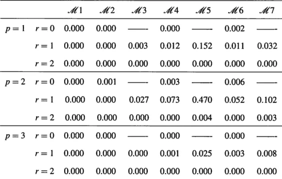
![Figure 2: Posterior expectation of the regime variable for 1 he US Term Structure of Interest rates 2 1.9 1.8 1.7 1.6 1.5 1.4 1.3 1.2 1.1 1 58 ! l~n j 64 rl ! I ~~ 70 76 Pr[St=211(t)] for f=6 and f=3 ~ ~ ,.T -- -~ ~' ~ 82 88 94 00 06 12](https://thumb-us.123doks.com/thumbv2/123dok_us/647375.2578033/28.873.193.683.667.1012/figure-posterior-expectation-regime-variable-term-structure-rates.webp)
