E
ff
ective Image Clustering based on Human Mental Search
Seyed Jalaleddin Mousavirad
1, Hossein Ebrahimpour-Komleh
1and Gerald Schaefer
21
Department of Electrical and Computer Engineering, University of Kashan, Iran
2Department of Computer Science, Loughborough University, U.K.
Abstract
Image segmentation is one of the fundamental techniques in image analysis. One group of segmentation techniques is based on clustering principles, where association of image pixels is based on a similarity criterion. Conventional clustering algorithms, such ask-means, can be used for this purpose but have several drawbacks including dependence on initialisation conditions and a higher likelihood of converging to local rather than global optima.
In this paper, we propose a clustering-based image segmentation method that is based on the human mental search (HMS) algorithm. HMS is a recent metaheuristic algorithm based on the manner of searching in the space of online auctions. In HMS, each candidate solution is called a bid, and the algorithm comprises three major stages: mental search, which explores the vicinity of a solution using Levy flight to find better solutions; grouping which places a set of candidate solutions into a group using a clustering algorithm; and moving bids toward promising solution areas. In our image clustering application, bids encode the cluster centres and we evaluate three different objective functions.
In an extensive set of experiments, we compare the efficacy of our proposed approach with several state-of-the-art metaheuristic algorithms including a genetic algorithm, differential evolution, particle swarm optimisation, artificial bee colony algorithm, and harmony search. We assess the techniques based on a variety of metrics including the objective functions, a cluster validty index, as well as unsupervised and supervised image segmentation criteria. Moreover, we perform some tests in higher dimensions, and conduct a statistical analysis to compare our proposed method to its com-petitors. The obtained results clearly show that the proposed algorithm represents a highly effective approach to image clustering that outperforms other state-of-the-art techniques.
Keywords:Image clustering, metaheuristic algorithms, human mental search, image segmentation.
1
Introduction
Image segmentation is a fundamental task in image processing and analysis. Image segmentation is the process of di-viding an image into several homogeneous meaningful areas. Pixels associated with a certain area, commonly described based on features such as colour or texture, exhibit more commonalities than those assigned to different areas. Image seg-mentation is employed in a variety of applications, such as satellite image analysis [1, 2], colour quantisation [3], tumour detection [4], food quality evaluation [5], and modelling of microstructures [6], to name a few.
is divided into a set of groups (clusters) so that the members of a group share more commonalities than those in different groups. This is typically achieved by optimising a criterion formulated as maximising the similarity among the members of a cluster, while ensuring that clusters are distinct from each other.
Thek-means algorithm is the most commonly employed clustering algorithm. Here, firstkcluster centres are defined randomly. Then, using a similarity criterion such as Euclidean distance, every pattern is assigned to its closest cluster centre. After that, the location of every cluster centre is recalculated. The process continues until a stopping condi-tion is satisfied. K-means is relatively simple but is also dependent on initialisation and converges to the closest local optimum [8].
Clustering can also be formulated as an optimisation problem. An optimisation problem is the problem of find-ing the minimum (or maximum) of an objective function in search space. Since many optimisation techniques have elements (such as initialisation) that introduce randomness, population-based metaheuristic algorithms, which use of mul-tiple solutions and their collaboration, can be employed for improved performance [8]. Metaheuristic algorithms are also problem-independent and can thus be used for a broad spectrum of optimisation problems. Using a series of operators, such algorithms try to direct a set of initially random solutions toward an appropriate area of the search space. Examples of population-based metaheuristic algorithms include genetic algorithms [9], particle swarm optimisation [10], differential evolution [11], bee colony algorithms [12], and harmony search [13].
In solving an optimisation problem using a metaheuristic algorithm, three significant issues should be taken into account: (1) the structure of a solution; (2) the objective function which determines the quality of a solution; and (3) the operators which cause the initial random solutions in search space to be directed to form better solutions. The operators have a crucial effect on the efficacy of a metaheuristic algorithm, so that the difference between metaheuristic algorithms is expressed by their different operators. Many studies have also been conducted to improve the effectiveness of different operators using new metaheuristic algorithms or extensions of existing algorithms for image segmentation [14–16].
One of the challenges in image clustering, compared with other applications, is that there is a large number of samples. For example, in a relatively small image of size 256×256, the number of samples (pixels) is 65,536, while an image of size 512×512 comprises 262,144 pixels. In the literature, various work has proposed the use of population-based metaheuristic algorithms for image clustering. For example, [17] used fuzzy c-means (FCM) and genetic algorithms (GAs) for image clustering with an objective function based on the total weighted squared error. This method showed a higher efficacy on satellite images compared with four algorithms including a self-organising map (SOM), a hybrid genetic algorithm (HGA), FCM, and a combination of SOM and HGA. [18] studied colour image segmentation using a GA and a SOM where the latter was used as a pre-processing operation to identify the number of clusters and an objective function based on compactness and separation. The obtained results indicated performance exceeding those of other state-of-the-art algorithms.
Particle swarm optimisation (PSO) [10, 19] is a population-based algorithm inspired by the social behaviour of birds. The first PSO-based image clustering algorithm is reported in [20]. Here, the structure of each particle is a single-dimensional array where every component corresponds to a cluster centre, and an error function was used as objective
ciples aims at avoiding local optima. The obtained results indicated that this method was able to outperform standard PSO. In [22], a bare-bones PSO (BPSO) algorithm was studied for image clustering. This approach does not require pa-rameter tuning, and good performance in comparison to other algorithms such ask-means and PSO was observed. Other PSO-based image clustering algorithms include [23–26], while other population-based metaheuristic algorithms such as differential evolution [27–29], bee colony algorithms [14, 30] and harmony search [31] have also been proposed for image clustering. Although these algorithms have shown satisfactory results in comparison with conventional algorithms, still better performance is required. Despite the diverse work done in this area, this is still a very active research subject with the aim of improving the efficacy of image clustering algorithms.
The human mental search (HMS) algorithm [32] is a relatively recent population-based algorithm which has demon-strated competitive performance for solving optimisation problems. Every solution in HMS is called a bid. The algorithm has three main operators. The first operator is mental search, which searches the vicinity of a solution using Levy flight. Levy flight, a type of random walk with varying step size, can simultaneously improve diversification and intensification. The second HMS operator is grouping which clusters the population with the aim of identifying promising areas in search space. Finally, the third operator instigates movement of solutions towards these promising areas.
According to the No Free Lunch (NFL) theorem [33] there is no best algorithm for solving an optimisation problem. This theorem is one of the main motivations for applying various metaheuristic algorithms for problems such as cluster-ing [27, 30, 31]. The HMS algorithm as a novel metaheuristic yielded satisfactory performance in comparison with other algorithms such as PSO, harmony search, and artificial bee colony algorithm [32].
Based on the NFL theorem and the competitive performance of HMS, in this paper, we propose a novel effective method for image clustering using the HMS algorithm. We define the structure of each HMS bid to be an array whose length equals the number of image clusters. For the optimisation, we investigate three objective functions, where the first two are based on intra-cluster distance, inter-cluster separation and quantisation error, while the third also incorporates a mean squared error criterion.
In an extensive set of experiments, we compare the efficacy of our proposed approach with several state-of-the-art metaheuristic algorithms including a genetic algorithm, differential evolution, particle swarm optimisation, artificial bee colony algorithm, and harmony search, and demonstrate it to exhibit excellent image clustering performance.
The remainder of the paper is organised as follows. Section 2 describes the concept of clustering, while Section 3 introduces the human mental search algorithm. Our proposed algorithm is described in Section 4, while experimental results are presented in Section 5. Finally, Section 6 concludes the paper.
2
Pattern clustering
The purpose of clustering is to group a set of patterns so that the members of each group have more similarity compared to intergroup members. Mathematically, clustering is defined as follows. Suppose, we have a set Pcomprising N d -dimensional patterns,P={p1,p2, . . . ,pn}. In the context of this paper, a pattern is equivalent to a pixel value. The aim of
clustering is to dividePintoKclustersC={c1,c2, . . . ,cK}so that the following conditions are satisfied:
2. The total number of patterns in all clusters is equal to the total number of patterns in the dataset:Sk
i=1ci=P;
3. Different clusters should not have mutual patterns:ciTcj=ϕ,i,j=1. . .K,i, j.
A criterion needs to be defined to be able to assess the clustering quality. The mean squared error (MSE) is the most common function for this purpose and defined as
f(P,C)= K X j=1 X Pi∈Cj d(pi,cj), (1)
whered(pi,cj) is the distance between patternpipattern and its cluster centercj. Several distance criteria can be used to
calculate the dissimilarity between patterns with the Euclidean distance
d(pi,pj)= v u t d X m=1 (pmi −pmj)2, (2) wherepm
i is them-th dimension ofpi, being the most popular one.
Thek-means algorithm is the best known and most employed algorithm in data clustering. It proceeds in the following steps:
Step 1: Randomly selectKpoints as cluster centres;
Step 2: Allocate each pattern to its closest cluster centre. More formally, ifC is the set of cluster centres, then each patternxis allocated to a cluster centre based on:
arg min
ci∈C
d(x,ci) (3)
wheredis the Euclidean distance;
Step 3: Recalculate the position of each cluster centre as the centroid of its allocated patterns as
ci= 1 |Si| X x∈Si x (4)
whereSiis thei-th cluster;
Step 4: Repeat Steps 2 and 3 until convergence (or until a different stopping criterion is met).
3
Human mental search
Human mental search [32] is a recently introduced population-based metaheuristic algorithm for solving optimisation problems. Every solution in HMS is called a bid and the algorithm is inspired by the manner of searching in a bid space of online auctions.
Algorithm 1HMS algorithm pseudo-code.
1: procedureHMS Algorithm
2: //Variables:L: lower bound;U: upper bound,Ml: minimum number of mental processes,Mh: maximum number
of mental processes,Npop: number of bids,Nvar: number of variables,K: number of clusters,iter: current iteration,
MaxIter: maximum number of iterations 3:
4: X=initialise population ofNpopbids
5: Calculate the objective function values of bids 6: x∗=find the best bid in the initial population 7: forifrom 1 toNpopdo
8: βi=generate integer random number betweenLandU
9: end for
10: foriterfrom 1 toMaxIterdo 11: //Mental search
12: forifrom 1 toNpopdo
13: qi=generate integer random number betweenMlandMh
14: end for
15: forifrom 1 toNpopdo
16: forjfrom 1 toqido
17: s=(2−iter∗(2/MaxIter))∗0.01∗ u
v1/βi ∗(xi−x∗)
18: NSj=Xi+s
19: end for
20: t=findNS with the lowest objective function value 21: ifcost(t)<cost(Xi)then
22: Xi=t
23: end if
24: end for
25: //Clustering
26: ClusterNpopbids intoKclusters
27: Calculate the mean objective function value of each cluster
28: Select cluster with lowest mean objective function value as the winner cluster 29: winner=select the best bid in the winner cluster
30: //Move bids toward best strategy 31: forifrom 1 toNpopdo
32: fornfrom 1 toNvardo
33: Xi
n=Xni+C∗(r∗winnern−Xni)
34: end for
35: end for
36: forifrom 1 toNpopdo
37: βi=generate random number betweenLandU
38: end for
39: x+=find best bid in current bids 40: ifcost(x+)<cost(x∗)then 41: x∗=x+
42: end if
43: end for
44: end procedure
3.1
Creating primary bids
Like other population-based algorithms, HMS commences by creating a set ofNpoprandom candidate solutions. Every
solution is called a bid. In ad-dimensional space, a bid is defined as
A bid is assessed using an objective function f() that evaluates the quality of a candidate solution:
f(bid)= f(x1,x2, ...,xd). (6)
3.2
Mental search
Mental search is one of the main operators introduced in the HMS algorithm. This operator creates a series of new solutions around each bid using a random walk in which the step size follows a Levy distribution. Compared to Brownian motion, use of the Levy distribution allows for improved diversification (due to ‘long jumps’) and intensification (due to ‘small steps’) and is thus more effective in exploring unknown spaces.
A new position is obtained as
NS =bid+S; (7)
withS is calculated as
S =(2−iter∗(2/MaxIter))∗α⊕Levy, (8)
whereMaxIteris the maximum number of iterations,iterindicates the current iteration, andαis a random number, while
⊕signifies element-wise multiplication. (2−iter∗(2/MaxIter)) is a descending factor, starting at 2 and ending towards 0, that considers a larger vicinity of a solution at the beginning and smaller vicinities at the end of the algorithm, thus yielding high diversification at the beginning and high intensification at the end.
The step sizeS using a Levy distribution is calculated as
S =(2−iter∗(2/MaxIter))∗α⊕Levy=(2−iter∗(2/MaxIter))∗0.01∗ u v1/β ∗(x
i−x∗), (9)
wherex∗is the best position found so far, anduandvare two random numbers with normal distributions as
u∼N(0, σ2u), v∼N(0, σ 2 v), (10) and σu= Γ(1+β) sin(πβ2) Γ[(1+2β)]β2(β−1)/2 1/β , σv=1, (11)
whereΓis a standard gamma function.
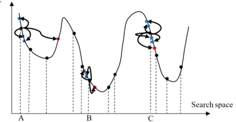
Figure 1 illustrates the mental search operator for two out of 12 existing bids (black dots) in the search space. The numbers of new bids created for bid A and B are 4 and 5 respectively (selected randomly). As can be seen, the vicinity of a solution is searched with the aim of finding better solutions (red and blue dots) and there are some ‘large jumps’. Finally, each bid is superseded with the best bid created by the mental search operator.
Figure 1: Example of mental search operator.
3.3
Grouping bids
The second operator in the HMS algorithm is a solution grouping operator using a clustering method. Bid clustering would cause solutions that are close to each other to be placed in one cluster. Here, thek-means clustering operator is used for bid clustering. After clustering, the mean objective function value is calculated for each cluster to determine promising areas in search space; an area with a lower mean objective value is likely a more appropriate area. Figure 2 illustrates the grouping operator. There are 12 bids in the figure, which are divided into three clusters. As can be seen, there are closer solutions in each cluster. This mechanism is different from most algorithms, which typically use the best solutions to identify promising areas in search space.
Figure 2: Example of bid grouping operator.
3.4
Moving towards the promising area
After grouping, the area with the lowest mean objective function value is selected as the winner group or the promising area. Then, the bids in the other groups move towards the best bid in this area. It is worth mentioning that the best bids among all bids may not belong to the winner group. Bids are updated as
t+1bid
n=tbidn+C∗(r×twinnern− tbid
wheret+1bid
nis then-th bid element at iterationt+1,twinnernis then-th element of the best bid in the winner group,tis
the current iteration,Cis a constant number, andris in [0; 1] derived from a normal distribution.
4
Image clustering using human mental search
In this paper, we propose an image clustering algorithm based on human mental search. For this, two issues to be determined are the structure of each bid and the objective function which we define in the following, before describing our proposed method step-by-step and working through an illustrative example.
4.1
Bid structure
In our approach, the structure of each bid is an array which encodes the centres of the clusters. The length of the array is equal toK withKthe number of clusters. The upper and lower bound of each bid are calculated asL =min(I) and
U = max(I) where Iis the image. In other words, the upper and lower bound are the minimum and maximum pixel values.
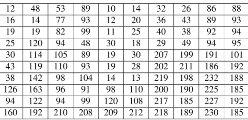
For illustration, Figure 3 displays a sample image of size 10×10.
12 48 53 89 10 14 32 26 86 88 16 14 77 93 12 20 36 43 89 93 19 19 82 99 11 25 40 38 92 94 25 120 94 48 30 18 29 49 94 95 30 114 105 89 19 30 207 199 191 101 43 119 110 93 19 28 202 211 186 192 38 142 98 104 14 13 219 198 232 188 126 163 96 91 98 110 200 190 225 185 94 122 94 99 120 108 217 185 227 192 160 192 210 208 209 212 218 189 230 185
Figure 3: Sample image.
Here,L=min(I) =10 andU =max(I)=232. Suppose that the number of clusters is 3. Hence, the length of each bid is 3 and an example of a bid would be (193,92,126).
4.2
Objective functions
Choosing an appropriate objective function is crucial for any population-based metaheuristic algorithm, since such al-gorithms update candidate solutions based on their quality as established by the objective function. In our work, we investigate three objective functions:
1. The first objective function [25] combines three factors expressing error, intra-cluster distance, and inter-cluster distance in a weighted form as
whereIis the image,bidis a bid defined asbid=[m1,m2, . . . ,mK] withmiindicating thei-th cluster centre,zmaxis the maximum data value (for an image of bitdepths,zmax=2s−1), andw1,w2, andw3are user-defined constants.
dmax(Z,bid), the intra-cluster distance, is calculated as
dmax(Z,bid)= max
j=1,...,K X ∀pi∈cj d(pi,bid) |cj| , (14)
whereKis the number of clusters,|cj|is the number of members of the j-th cluster, andd(pi,bid) is the Euclidean
distance betweenpiandbid.
The inter-cluster separationdmin(bid), which is based on the minimum average Euclidean distance between a pair of clusters and should be maximised, is defined as
dmin(bid)= min
∀i,j,i,j(d(mi,mj)). (15)
The quantisation errorJeis calculated as
Je= PK j=1 P ∀pi∈cjd(pi,bid)/|cj| K . (16)
Following [14], we setw1,w2, andw3to 0.4, 0.2, and 0.4, respectively.
2. To avoid having to find appropriate values forw1,w2, andw3, the second objective function [22] is defined as
CF2(bid,I)= dmax(I,bid)+Je
dmin(I,bid)
. (17)
3. The third objective function [14] is defined as
CF3(bid,I)=Je×
dmax(I,bid)
dmin(I,bid)
×(dmax(I,bid)+zmax−dmin(I,bid)+MS E), (18) whereMS E, the mean squared error, is calculated as
MS E= 1 N K X j=1 X ∀zp∈Cj d(zp,bid)2, (19)
withNindicating the total number of samples (pixels).
4.3
Proposed algorithm
Our proposed image clustering algorithm proceeds in the following steps:
Step 1: Parameter initialisation: the parameters include the number of clusters for image segmentationK, the number of bidsN, the number of clusters for bid groupingKH MS, the minimum and maximum number of mental searches
Step 2: Create an initial population as population= bid1 bid2 ... bidN , (20) wherebidi=[m1,m2, ...,mK].
Step 3: Calculate the value of the objective function for each bid. Step 4: Select the bid with the best objective function value.
Step 5: Select a random number betweenMlandMhfor each bid to define the number of mental searches for each bid.
Step 6: Mental search operator: create new bids in the vicinity of existing bids using a Levy distribution. This operation is carried out using Equations (7) and (9).
Step 7: Replacement operator: in case a new bid is better than a previous one it will replace the latter. Step 8: Bid grouping: the bid population is clustered using thek-means algorithm.
Step 9: Calculate the objective function value for each cluster member.
Step 10: The cluster with the minimum mean objective function value is selected as the winner cluster indicating a promis-ing area.
Step 11: Other bids move toward the best bid available in the winner group based on Equation (12).
Step 12: Find the best bidbid+among all bids and if it is better than the previous best bidbid∗replacebid∗with it. Step 13: If the stop condition is not satisfied, go back to Step 3.
4.4
An illustrative example
We illustrate the workings of our proposed algorithm using a simplified example based on the image defined in Figure 3. As the image size is 10×10, there are 100 samples in the image. Suppose that we want to divide the image into 3 clusters, i.e. K = 3. In this example, our goal is to minimise the first of the three objective functions, i.e.CF1 as defined in Equation (13). As parameters, we setN=12,KH MS =3,Ml=2, andMh=10.
Table 1: Initial population.
bid objective function value number of mental searches
(120.34, 229.38, 41.76) 39.26 2 (88.59, 127.41, 162.08) 49.52 5 (124.51, 30.15, 222.87) 35.51 2 (109.08, 82.61, 18.05) 52.09 8 (123.96, 188.78, 217.79) 50.38 4 (117.61, 114.31, 197.44) 55.74 2 (36.92, 43.58, 157.33) 55.32 4 (191.46, 190.55, 203.70) 58.66 3 (101.29, 35.81, 15.76) 51.93 7 (41.14, 160.28, 196.78) 50.64 2 (144.16, 47.80, 136.06) 56.42 5 (197.55, 96.06, 146.38) 46.27 7
We calculate the CF1 objective function value for the first bid, i.e. for (120.34, 229.38, 41.76), as
dmax(Z,bid) = max
j=1,...,K X ∀pi∈Cj d(pi,bid) |Cj| =max(4.04,5.61,3.37)=5.61 (21) D = ∞ 109.04 78.58 109.04 ∞ 187.62 78.58 187.62 ∞ (22)
dmin(bid) = min
∀i,j,i,j(d(mi,mj))=min(D)=78.58 (23) Je = PK j=1 P ∀pi∈cjd(pi,bid)/|cj| K = 4.0398+5.6108+3.3658 5 =4.34 (24) (25) and
CF1(bid,I)=w1dmax(Z,bid)+w2(zmax−dmin(I,bid))+w3Je=0.4×5.61+0.2×(255−78.58)+0.4×4.34=39.26. (26)
The objective function values for the other bids are calculated equivalently and are listed in Table 1. From this, we obtainbid∗=(124.51,30.15,222.87) as the best bid.
Table 1 also shows the numbers of mental searches assigned for each bid, which were randomly drawn from [Ml,Mh]=
[2; 10].
We next use the mental search operator on the bids. For the first bid, this gives:
stepsize=0.01×step×((120.34,229.38,41.76)−(124.51,30.15,222.87))=(−0.0049,6.9362,−0.5802) (27)
newbid=((120.34,229.38,41.76)+(2−iter∗(2/maxiter))∗stepsize=(120.33,243.11,40.61) (28)
while another new bid is calculated for the second mental search of this candidate solution in the same fashion and the same operations performed to obtain new bids for all other solutions.
If an improved bid is found it replaces the previous candidate solution leading to a new set of bids that is listed in Table 2. As can be seen, for all bids the objective function values either improves or stays the same.
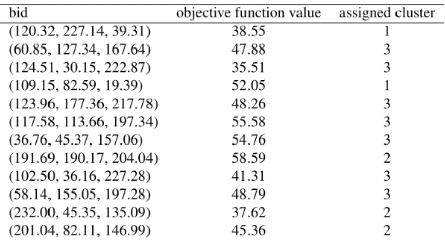
Table 2: Population after mental search operations.
bid objective function value assigned cluster
(120.32, 227.14, 39.31) 38.55 1 (60.85, 127.34, 167.64) 47.88 3 (124.51, 30.15, 222.87) 35.51 3 (109.15, 82.59, 19.39) 52.05 1 (123.96, 177.36, 217.78) 48.26 3 (117.58, 113.66, 197.34) 55.58 3 (36.76, 45.37, 157.06) 54.76 3 (191.69, 190.17, 204.04) 58.59 2 (102.50, 36.16, 227.28) 41.31 3 (58.14, 155.05, 197.28) 48.79 3 (232.00, 45.35, 135.09) 37.62 2 (201.04, 82.11, 146.99) 45.36 2
Next, the bids are grouped intoKH MS clusters using thek-means algorithm. The result of this is also shown in Table 2
where for each bid the resulting cluster number (1, 2 or 3) is given. As we can see, there are 2 bids in cluster 1, 3 bids in cluster 2, and 8 bids in cluster 3. The mean objective function values for the three clusters are 45.30, 47.19, and 47.44, respectively. Yielding the lowest value, cluster 1 is thus the winner cluster.
The best bid in cluster 1 is (120.32, 227.14, 39.31) with an objective function value of 38.55. As can be seen, this bid is not the best existing bid as there exists one with an objective function value of 35.51. Finally, the other bids will move toward the winner bid. For example the current bid (36.76, 45.37, 157.06) is updated as
(36.76,45.37,157.06)+2∗((0.7,0.3,0.4)×((120.32,227.14,39.31)−(36.76,45.37,157.06))=(153.74,154.43,62.86),
(29) and the other bids are updated in the same fashion.
This concludes the first iteration of the algorithm and the same process will continue until a stopping criterion is met.
5
Experimental results
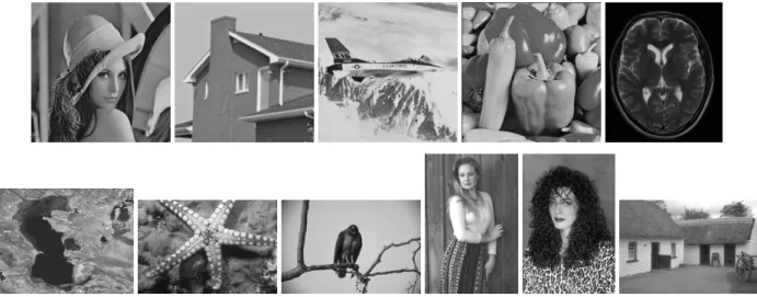
In order to evaluate our proposed image clustering algorithm, we ran an extensive set of experiments. The 11 images that we employed for this purpose, shown in Figure 4, are commonly used for image clustering evaluation: Lenna, House, Airplane, Peppers, MRI and Caspian Sea, and five images from the Berkeley segmentation dataset [34], namely 12003, 42049, 181079, 198054, and 385028.
We compared our proposed algorithm with a number of population-based clustering algorithms that have been previ-ously used for image clustering, including genetic algorithm-based clustering (GA), differential evolution-based clustering (DE), particle swarm optimisation-based clustering (PSO), artificial bee colony algorithm-based clustering (ABC), and harmony search-based clustering (HS), as well as with thek-means clustering algorithm.
Figure 4: The test image dataset.
5 [14]. Each algorithm was run 50 times and in all instances we report the average results over these 50 runs. Table 3: Parameter settings for all algorithms.
algorithm parameters value
GA crossover probability 0.8
mutation probability 1/(number of thresholds)
DE [11] scaling factor 0.5
crossover probability 0.1
PSO [36] cognitive constant 2
social constant 2
inertia constant 1 to 0
ABC [35] limit ne×dimension of problem
HS [13] harmony memory considering rate 0.9
pitch adjusting rate 0.1
HMS number of clusters 5
C 2
5.1
Objective functions
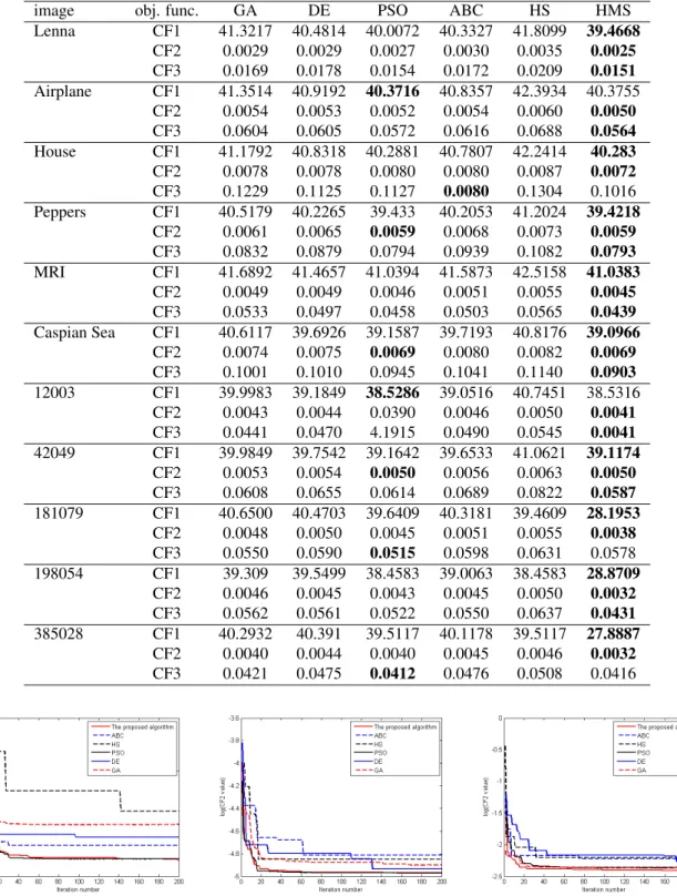
As mentioned above, we are considering three different objective functions. Table 4 gives the obtained results for the three objective functions for all images and algorithms.
As we can see from Table 4, our proposed method consistently leads to better objective function values compared to all other algorithms, confirming its higher efficacy. PSO achieved the best result for Airplane and 12003 based on the CF1 objective function and gives similar CF2 results to HMS for Pepper, Caspian Sean and 42049. ABC shows the best results for House based on CF3, whereas for this objective function PSO yields the best performance for 181079 and 385028. In all other cases, our proposed HMS image clustering algorithm provides the best objective function results.
We also investigated the convergence speed for all algorithms. Figure 5 shows plots of the objective function values against the number of iterations on the Caspian Sea image (other images showed similar results). As can be seen, our approach leads to faster convergence compared to other algorithms.
Table 4: Objective function results for all imaged and algorithms. Best results for an image are bolded.
image obj. func. GA DE PSO ABC HS HMS
Lenna CF1 41.3217 40.4814 40.0072 40.3327 41.8099 39.4668 CF2 0.0029 0.0029 0.0027 0.0030 0.0035 0.0025 CF3 0.0169 0.0178 0.0154 0.0172 0.0209 0.0151 Airplane CF1 41.3514 40.9192 40.3716 40.8357 42.3934 40.3755 CF2 0.0054 0.0053 0.0052 0.0054 0.0060 0.0050 CF3 0.0604 0.0605 0.0572 0.0616 0.0688 0.0564 House CF1 41.1792 40.8318 40.2881 40.7807 42.2414 40.283 CF2 0.0078 0.0078 0.0080 0.0080 0.0087 0.0072 CF3 0.1229 0.1125 0.1127 0.0080 0.1304 0.1016 Peppers CF1 40.5179 40.2265 39.433 40.2053 41.2024 39.4218 CF2 0.0061 0.0065 0.0059 0.0068 0.0073 0.0059 CF3 0.0832 0.0879 0.0794 0.0939 0.1082 0.0793 MRI CF1 41.6892 41.4657 41.0394 41.5873 42.5158 41.0383 CF2 0.0049 0.0049 0.0046 0.0051 0.0055 0.0045 CF3 0.0533 0.0497 0.0458 0.0503 0.0565 0.0439 Caspian Sea CF1 40.6117 39.6926 39.1587 39.7193 40.8176 39.0966 CF2 0.0074 0.0075 0.0069 0.0080 0.0082 0.0069 CF3 0.1001 0.1010 0.0945 0.1041 0.1140 0.0903 12003 CF1 39.9983 39.1849 38.5286 39.0516 40.7451 38.5316 CF2 0.0043 0.0044 0.0390 0.0046 0.0050 0.0041 CF3 0.0441 0.0470 4.1915 0.0490 0.0545 0.0041 42049 CF1 39.9849 39.7542 39.1642 39.6533 41.0621 39.1174 CF2 0.0053 0.0054 0.0050 0.0056 0.0063 0.0050 CF3 0.0608 0.0655 0.0614 0.0689 0.0822 0.0587 181079 CF1 40.6500 40.4703 39.6409 40.3181 39.4609 28.1953 CF2 0.0048 0.0050 0.0045 0.0051 0.0055 0.0038 CF3 0.0550 0.0590 0.0515 0.0598 0.0631 0.0578 198054 CF1 39.309 39.5499 38.4583 39.0063 38.4583 28.8709 CF2 0.0046 0.0045 0.0043 0.0045 0.0050 0.0032 CF3 0.0562 0.0561 0.0522 0.0550 0.0637 0.0431 385028 CF1 40.2932 40.391 39.5117 40.1178 39.5117 27.8887 CF2 0.0040 0.0044 0.0040 0.0045 0.0046 0.0032 CF3 0.0421 0.0475 0.0412 0.0476 0.0508 0.0416
Figure 5: Convergence behaviour of all algorithms on Caspian Sea image for CF1 (left), CF2 (middle) and CF3 (right) objective functions.
5.2
Clustering validity
Clustering validity indices are metrics that indicate clustering quality. In general, they assess two aspects of clustering: 1. Compactness: to the extent possible, samples in a cluster should be similar.
clustering validity indices. The DB index measures the proportion of within-cluster scatter to between-cluster separation. The scatter within thei-th cluster is calculated as
Si= 1 Ni X xj∈ci d(xj,mi), (30)
whereNiis the number of samples of thei-th clusterci, andd(xj,mi) is the Euclidean distance between samplexjand its
cluster centremi. The between-cluster separation is calculated as
Ri j =
Si+Sj
d(mi,mj)
,i, j. (31)
Finally, the DB index is defined as
DB= 1 K K X k=1 Rk, (32)
whereRk=maxj=1,2,...,KRi jandi=1,2, ...,K.
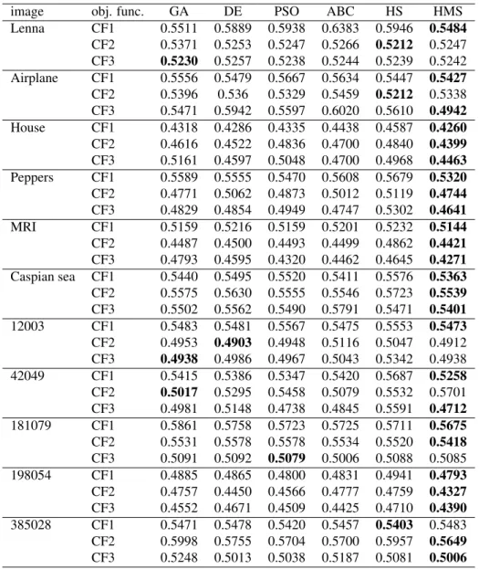
Table 5 reports the average DB results over the 50 runs for all three objective functions. As we can see, in 26 out of 33 cases, our proposed approach yields the best (i.e., lowest) DB index.
5.3
Non-parametric statistical analysis
Due to the randomness and variance of population-based metaheuristic algorithms, we also conducted a non-parametric statistical analysis. The null hypothesisH0here means that there is no statistical difference between two algorithms, while the alternative hypothesisH1 indicates a statistically significant difference between the algorithms. The null hypothesis is the initial statistical claim and if the null hypothesis is rejected the alternative one would be accepted. We utilised two well-known non-parametric tests, namely the Friedman test and the Wilcoxon signed rank test to compare the different image clustering algorithms.
The first stage of the Friedman test is rank calculation for which we list the results in Table 6. As is evident, our proposed algorithm has the lowest average rank with PSO coming second. The chi-squared value and p-value were evaluated as 110.91 and 2.630e-22 respectively. Given the table of chi-squared distribution, the critical value for the degree of freedom (6-1=5) andα = 0.05 is equal to 11.070. The chi-squared value is higher which means thatH1 is accepted. In other words, there is a statistical difference between the algorithms. Moreover, the p-value is extremely small which confirms the rejection ofH0.
The result (p-value) of the Wilcoxon signed rank test determines the significance level between two algorithms. If the p-value is less than 0.05, there would be a significant statistical difference between the algorithms. Table 7 reports the obtained results of the Wilcoxon test. As can be seen, there is a significant difference between our proposed algorithm and all other algorithms, with all obtained p-values less than 0.05.
Table 5: DB index results for all images and all algorithms. The best result for each image is bolded.
image obj. func. GA DE PSO ABC HS HMS
Lenna CF1 0.5511 0.5889 0.5938 0.6383 0.5946 0.5484 CF2 0.5371 0.5253 0.5247 0.5266 0.5212 0.5247 CF3 0.5230 0.5257 0.5238 0.5244 0.5239 0.5242 Airplane CF1 0.5556 0.5479 0.5667 0.5634 0.5447 0.5427 CF2 0.5396 0.536 0.5329 0.5459 0.5212 0.5338 CF3 0.5471 0.5942 0.5597 0.6020 0.5610 0.4942 House CF1 0.4318 0.4286 0.4335 0.4438 0.4587 0.4260 CF2 0.4616 0.4522 0.4836 0.4700 0.4840 0.4399 CF3 0.5161 0.4597 0.5048 0.4700 0.4968 0.4463 Peppers CF1 0.5589 0.5555 0.5470 0.5608 0.5679 0.5320 CF2 0.4771 0.5062 0.4873 0.5012 0.5119 0.4744 CF3 0.4829 0.4854 0.4949 0.4747 0.5302 0.4641 MRI CF1 0.5159 0.5216 0.5159 0.5201 0.5232 0.5144 CF2 0.4487 0.4500 0.4493 0.4499 0.4862 0.4421 CF3 0.4793 0.4595 0.4320 0.4462 0.4645 0.4271 Caspian sea CF1 0.5440 0.5495 0.5520 0.5411 0.5576 0.5363 CF2 0.5575 0.5630 0.5555 0.5546 0.5723 0.5539 CF3 0.5502 0.5562 0.5490 0.5791 0.5471 0.5401 12003 CF1 0.5483 0.5481 0.5567 0.5475 0.5553 0.5473 CF2 0.4953 0.4903 0.4948 0.5116 0.5047 0.4912 CF3 0.4938 0.4986 0.4967 0.5043 0.5342 0.4938 42049 CF1 0.5415 0.5386 0.5347 0.5420 0.5687 0.5258 CF2 0.5017 0.5295 0.5458 0.5079 0.5532 0.5701 CF3 0.4981 0.5148 0.4738 0.4845 0.5591 0.4712 181079 CF1 0.5861 0.5758 0.5723 0.5725 0.5711 0.5675 CF2 0.5531 0.5578 0.5578 0.5534 0.5520 0.5418 CF3 0.5091 0.5092 0.5079 0.5006 0.5088 0.5085 198054 CF1 0.4885 0.4865 0.4800 0.4831 0.4941 0.4793 CF2 0.4757 0.4450 0.4566 0.4777 0.4759 0.4327 CF3 0.4552 0.4671 0.4509 0.4425 0.4710 0.4390 385028 CF1 0.5471 0.5478 0.5420 0.5457 0.5403 0.5483 CF2 0.5998 0.5755 0.5704 0.5700 0.5957 0.5649 CF3 0.5248 0.5013 0.5038 0.5187 0.5081 0.5006
Table 6: Ranks for all algorithms. algorithm average rank
GA 3.8636 DE 3.8788 PSO 2.3182 ABC 4.1061 HS 5.6061 HMS 1.2273
Table 7: Results of Wilcoxon signed rank test. p-value HMS vs. GA 2.0905e-06 HMS vs. DE 5.3525e-05 HMS vs. PSO 2.8234e-04 HMS vs. ABC 3.8488e-06 HMS vs. HS 5.3720e-07
Table 8: Standard deviations for all images and algorithms. The best result for each image is bolded.
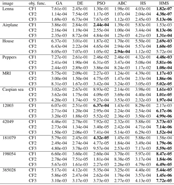
image obj. func. GA DE PSO ABC HS HMS
Lenna CF1 7.61e-01 2.45e-01 1.30e-01 1.98e-01 4.03e-01 1.82e-07 CF2 1.14e-04 7.54e-05 1.17e-05 1.07e-04 2.04e-04 4.38e-07 CF3 1.69e-03 6.73e-04 7.67e-05 1.12e-03 2.45e-03 5.13e-06 Airplane CF1 3.86e-01 2.84e-01 2.44e-04 1.39e-01 5.83e-01 1.53e-03 CF2 2.16e-04 1.19e-04 2.55e-04 1.00e-04 3.44e-04 8.13e-06 CF3 2.35e-03 8.72e-04 4.84e-04 1.25e-03 4.21e-03 1.31e-04 House CF1 6.37e-01 3.01e-01 1.87e-02 1.70e-01 5.50e-01 2.69e-03 CF2 6.43e-04 2.22e-04 4.65e-04 2.94e-04 5.57e-04 1.60e-05 CF3 8.05e-03 7.07e-03 1.05e-02 2.94e-04 1.12e-02 5.72e-04 Peppers CF1 7.27e-01 2.61e-01 2.46e-02 2.46e-01 4.32e-01 4.48e-03 CF2 2.41e-04 1.90e-04 6.31e-05 3.47e-04 5.08e-04 5.81e-06 CF3 2.44e-03 2.89e-03 3.86e-04 8.24e-03 1.17e-02 1.08e-04 MRI CF1 5.75e-01 2.09e-01 2.27e-03 1.24e-01 4.39e-01 1.17e-03 CF2 3.00e-04 1.50e-04 4.75e-05 1.47e-04 2.33e-04 1.86e-06 CF3 8.31e-03 1.67e-03 3.42e-04 3.24e-03 3.05e-03 5.02e-05 Caspian sea CF1 3.02e-01 2.67e-01 8.93e-02 2.14e-01 3.98e-01 1.61e-03 CF2 3.62e-04 1.75e-04 4.09e-05 3.69e-04 4.40e-04 1.01e-05 CF3 4.20e-03 1.74e-03 9.27e-04 3.53e-03 2.32e-03 1.97e-04 12003 CF1 6.07e-01 2.51e-01 6.37e-04 1.43e-01 8.29e-01 2.17e-03 CF2 2.71e-04 1.20e-04 2.95e-04 2.24e-04 2.54e-04 6.17e-06 CF3 3.20e-03 1.88e-03 5.52e-02 2.36e-03 3.50e-03 4.99e-06 42049 CF1 4.46e-01 2.78e-01 7.92e-02 2.32e-01 5.88e-01 3.73e-03 CF2 2.73e-04 1.34e-04 3.40e-05 2.42e-04 4.71e-04 7.14e-06 CF3 1.50e-03 2.06e-03 7.41e-04 5.14e-03 6.29e-03 1.52e-04 181079 CF1 5.79e-01 2.45e-01 4.32e-05 1.45e-01 5.88e-01 1.58e-04 CF2 2.49e-04 2.74e-04 4.77e-05 1.84e-04 3.49e-04 1.79e-06 CF3 4.80e-03 3.78e-03 9.57e-04 2.53e-03 7.17e-03 5.59e-05 198054 CF1 6.60e-01 3.60e-01 2.60e-04 3.70e-01 5.97e-01 8.47e-05 CF2 2.78e-04 7.51e-05 1.81e-04 8.38e-05 3.17e-04 1.84e-06 CF3 5.67e-03 1.61e-03 2.27e-03 2.26e-03 4.79e-03 6.49e-05 385028 CF1 5.17e-01 4.12e-01 5.35e-04 3.25e-01 4.40e-01 5.44e-05 CF2 5.86e-05 2.47e-04 2.62e-04 1.76e-04 3.57e-04 1.45e-06 CF3 3.10e-03 3.17e-03 3.73e-03 2.77e-03 4.13e-03 7.72e-05
5.4
Stability analysis
Due to the randomness of metaheuristic algorithms, each run of an algorithm will generate a different result. A lower dispersion among multiple runs of an algorithm hence indicates a more stable algorithm. We therefore analyse the stability of the evaluated techniques and employ the standard deviation
S T D= v u tM X i=1 (xi−µ)2 M , (33)
whereMis the number of runs (M =50 in our experiments),xiis the objective function value obtained for thei-th run
andµis the mean objective function value for the algorithm.
Table 8 lists the obtained results. As can be seen, in all but 4 cases, our proposed method yields the lowest standard deviation, which demonstrates that our approach is more stable in comparison with other metaheuristic-based image clustering techniques.
5.5
Comparison with conventional clustering-based methods
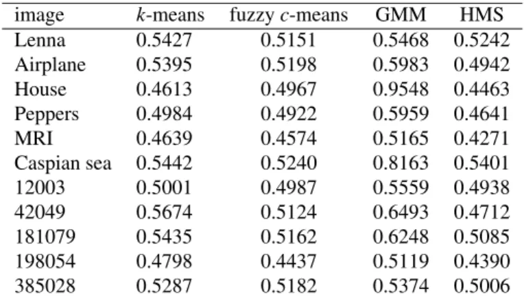
In addition to comparing our proposed HMS-based algorithm to image clustering based on other metaheuristic optimisation-based approaches, we also compared its performance to conventional clustering-optimisation-based methods, namelyk-means, fuzzy
c-means, and Gaussian mixture model (GMM). We perform this, employing the CF3 objective function for HMS and using the DB index as evaluation criterion. The results are given in Table 9 which shows that our approach clearly out-performs the other algorithms in most cases. We also performed a Wilcoxon signed rank test to compare the methods; Table 10 confirms that our HMS algorithm is statistically significantly better than the other approaches.
Table 9: DB index results of conventional clustering-based methods and HMS. image k-means fuzzyc-means GMM HMS
Lenna 0.5427 0.5151 0.5468 0.5242 Airplane 0.5395 0.5198 0.5983 0.4942 House 0.4613 0.4967 0.9548 0.4463 Peppers 0.4984 0.4922 0.5959 0.4641 MRI 0.4639 0.4574 0.5165 0.4271 Caspian sea 0.5442 0.5240 0.8163 0.5401 12003 0.5001 0.4987 0.5559 0.4938 42049 0.5674 0.5124 0.6493 0.4712 181079 0.5435 0.5162 0.6248 0.5085 198054 0.4798 0.4437 0.5119 0.4390 385028 0.5287 0.5182 0.5374 0.5006
Table 10: Results of Wilcoxon signed rank test between HMS and conventional clustering-based methods.
algorithms p-value
HMS vs.k-means 9.7656e-04 HMS vs. fuzzyc-means 0.0322 HMS vs. GMM 9.7656e-04
5.6
Search ability in high dimensions
The curse of dimensionality is a well-known problem that can occur when employing optimisation-based algorithms, since increasing the dimensionality of a problem exponentially expands the search space. In our image clustering problem, dimensionality primarily relates to the number of clusters (image regions) for which the algorithm tries to identify the best configuration.
In Table 11 we hence report results with different numbers of clusters, namelyK ={5,10,15}. As can be seen from there, under all settings our proposed algorithm outperforms all other approaches. Only in 5 out of the 33 cases, one of the other algorithms gives a better clustering result, while this happens only once each for the more difficult cases ofK=10 andK=15 indicating that our approach scales better with regards to the dimensionality of the problem compared to other techniques.
The superiority of our approach is also confirmed in Tables 12 and 13 which give the results of the Friedman and Wilcoxon test forK = 10 and K = 15 respectively. Both tests confirm that the proposed HMS algorithm performs statistically significantly better than the other metaheuristics (with the exception of HMS vs. PSO forK=10).
Table 11: Obtained results for different numbers of clusters. The best results for each case are bolded.
image K GA DE PSO ABC HS HMS
Lenna 5 0.0169 0.0178 0.0154 0.0172 0.0209 0.0151 10 0.0271 0.0323 0.0353 0.0617 0.0619 0.0222 15 0.0349 0.0548 0.0463 0.1212 0.1087 0.0348 Airplane 5 0.0604 0.0605 0.0572 0.0616 0.0688 0.0564 10 0.0894 0.1110 0.1310 0.1204 0.1486 0.0775 15 0.1239 0.1793 0.1107 0.2692 0.2688 0.0974 House 5 0.1229 0.1125 0.1127 0.0080 0.1304 0.1016 10 0.2981 0.3062 0.2780 0.5316 0.4275 0.2023 15 0.3400 0.6739 0.4209 1.0115 1.0126 0.3260 Peppers 5 0.0832 0.0879 0.0794 0.0939 0.1082 0.0793 10 0.1564 0.1664 0.1292 0.2140 0.2505 0.1104 15 0.3665 0.2109 0.2998 0.4263 0.4255 0.1363 MRI 5 0.0533 0.0497 0.0458 0.0503 0.0565 0.0439 10 0.0831 0.1064 0.0658 0.1227 0.1416 0.0657 15 0.1604 0.1431 0.1575 0.2851 0.2785 0.0817 Caspian sea 5 0.1001 0.1010 0.0945 0.1041 0.1140 0.0903 10 0.2886 0.2562 0.2745 0.3417 0.4807 0.2046 15 0.5903 1.0795 0.4828 2.0182 2.0531 0.6128 12003 5 0.0441 0.0470 4.1915 0.0490 0.0545 0.0041 10 0.0791 0.0844 0.0658 0.1516 0.1207 0.0590 15 0.1229 0.1499 0.1095 0.2627 0.2025 0.0830 42049 5 0.0608 0.0655 0.0614 0.0689 0.0822 0.0587 10 0.0985 0.1244 0.0853 0.1617 0.1390 0.0783 15 0.1426 0.1739 0.1414 0.4123 0.4626 0.0990 181079 5 0.0550 0.0590 0.0515 0.0598 0.0631 0.0578 10 0.0896 0.1250 0.0956 0.1764 0.1756 0.0875 15 0.1494 0.1594 0.1423 0.1875 0.2710 0.1179 198054 5 0.0562 0.0561 0.0522 0.0550 0.0637 0.0431 10 0.1131 0.1517 0.0974 0.1847 0.1767 0.0982 15 0.2263 0.2616 0.1729 0.3315 0.3740 0.1522 385028 5 0.0421 0.0475 0.0412 0.0476 0.0508 0.0416 10 0.0626 0.0900 0.0599 0.0989 0.1125 0.0599 15 0.1143 0.1430 0.0871 0.2491 0.2139 0.0114 Table 12: Results of Friedman tests forK=10 andK=15
algorithm average rankK=10 average rankK=15
GA 2.82 2.91 DE 3.64 3.64 PSO 2.50 2.27 ABC 5.36 5.55 HS 5.55 5.45 HMS 1.13 1.18 chi-squared 33.79 47.94
p-value 7.5068e-09 3.6620e-09
Table 13: Results of Wilcoxon signed rank tests forK=10 andK=15. p-valueK=10 p-valueK=15
HMS vs. GA 9.7565e-04 0.0049 HMS vs. DE 9.7565e-04 9.7565e-04
HMS vs. PSO 0.0059 0.0420
HMS vs. ABC 9.7565e-04 9.7565e-04 HMS vs. HS 9.7565e-04 9.7565e-04
5.7
Parameter settings
Like every metaheuristic algorithm, HMS also has some parameters which in turn affect the performance of the algorithm. While in the experiments above, we have selected default values for the HMS parameters, in our next experiment we investigated the behaviour of our algorithm with respect to the two main parameters of the algorithm, namely the number of clusters for bid groupingKH MS, and the number of mental searches.
Our analysis is inspired by [32, 38], and we selected two images, House and Peppers, and the CF3 objective function for this purpose. The House image was chosen as here, for the CF3 function, HMS did not provide the best result, while for Peppers our approach yielded the best performance.
5.7.1 Number of clusters for grouping bids
As mentioned in [32], more local optima might require a higher number of clusters. Figure 6 illustrates the effect of the number of clusters on the mean objective function value. As can be seen, by increasing the number of clusters for the House image, the mean objective function value decreases, while similar results, though on a smaller scale, are observed for the Pepper image. This indicates that the number of clusters can have a considerable effect on the efficacy of the algorithm and lead to improved clustering performance.
Figure 6: Number of clusters for bid grouping vs. mean objective function value for House (left) and Peppers (right)
5.7.2 Number of mental searches
As mentioned, the number of mental searches is randomly selected between the user-defined lower (L) and upper (H) limit. We therefore asses the algorithm’s sensitivity to different settings of this interval. The results are given in Figure 7. As can be observed from there, an increased number of mental searches will in general lead to better image clustering performance.
5.8
Image segmentation performance
Last not least, we evaluated the performance of our proposed algorithm in terms of image segmentation quality. Clearly this is crucial, since image clustering is primarily employed for the purpose of segmentation. For this, we used three unsupervised and two supervised image segmentation criteria from the literature. While unsupervised criteria do not require a manually-segmented ground truth images, this is necessary for supervised criteria. As only the images of the Berkeley segmentation dataset come with such a ground truth, the experiments for supervised criteria were conducted only on these images, i.e. images 12003, 42049, 181079, 198054, and 385028.
The Borsotti criterion (BOR) [39] is an unsupervised segmentation metric derived from the number, the variance, and the area of segmented image regions, with a lower BOR indicating better segmentation performance. Tables 14 shows the BOR results for all algorithms on the test image set. As we can see, for 8 of the 11 images, our HMS approach affords the best BOR results. This is further confirmed in the calculated rankings of the algorithms, which is also given in Table 14.
Table 14: BOR results for all images and all algorithms. Best results are bolded.
image GA DE PSO ABC HS HMS
Lenna 0.0210 0.0204 0.0197 0.0205 0.0220 0.0196 Airplane 0.0208 0.0204 0.0196 0.0205 0.0196 0.0190 House 0.0188 0.0174 0.0182 0.0197 0.0191 0.0169 Peppers 0.0282 0.0287 0.0274 0.0300 0.0301 0.0275 MRI 0.0158 0.0130 0.0130 0.0132 0.0142 0.0128 Caspian Sea 0.0299 0.0304 0.0286 0.0291 0.0301 0.0292 12003 0.0359 0.0358 0.0360 0.0362 0.0377 0.0358 42049 0.0149 0.0147 0.0141 0.0152 0.0160 0.0140 181079 0.0561 0.0571 0.0548 0.056 0.0554 0.0551 198054 0.0710 0.0761 0.0704 0.0692 0.0704 0.0691 385028 0.0674 0.0679 0.0670 0.0671 0.0677 0.0663 average rank 4.45 4.00 2.23 4.09 4.82 1.41
Another unsupervised criterion used to evaluate image segmentation performance is Levine and Nazif’s interclass contrast (LNIC) [40]. This criterion calculates the sum of region contrasts weighted by their areas, with a higher LNIC value signifying better performance. Table 15 summarises the obtained LNIC results for all algorithms. As we can see, our proposed approach yields the best result in 9 of the 11 cases and is clearly ranked first among the 6 approaches.
Table 15: LNIC results for all images and all algorithms. Best results are bolded.
image GA DE PSO ABC HS HMS
Lenna 0.2391 0.2368 0.2368 0.2381 0.2405 0.2596 Airplane 0.1241 0.1207 0.1229 0.1242 0.1211 0.1243 House 0.1715 0.1834 0.1731 0.1703 0.1743 0.1785 Peppers 0.2592 0.2590 0.2597 0.2609 0.2598 0.2599 MRI 0.6202 0.6260 0.6254 0.6226 0.6236 0.6283 Caspian Sea 0.2134 0.2131 0.2132 0.2122 0.2120 0.2139 12003 0.2607 0.2607 0.2602 0.2606 0.2591 0.2616 42049 0.2492 0.2505 0.2513 0.2411 0.2531 0.2577 181079 0.2343 0.2437 0.2344 0.2387 0.2401 0.2885 198054 0.4381 0.4345 0.4319 0.4310 0.4376 0.5207 385028 0.2022 0.2032 0.2028 0.2060 0.2048 0.2572 average rank 4.14 3.73 4.23 4.09 3.64 1.18
nor-malised standard deviations of the image regions. A higher LNIU value indicates better segmentation performance. For 8 of the 11 images, the proposed HMS algorithm achieves the best LNIU result and is thus also ranked first overall.
Table 16: LNIU results for all images and all algorithms. Best results are bolded.
image GA DE PSO ABC HS HMS
Lenna 0.0329 0.0323 0.0314 0.0322 0.0338 0.0586 Airplane 0.0333 0.0354 0.0341 0.0343 0.0335 0.0392 House 0.0228 0.0265 0.0233 0.0236 0.0233 0.0256 Peppers 0.0395 0.0399 0.0398 0.0392 0.0392 0.0399 42049 0.0353 0.0356 0.0346 0.0359 0.0364 0.0359 12003 0.0526 0.0529 0.0521 0.0534 0.0534 0.0535 181079 0.0486 0.0506 0.0489 0.0497 0.0489 0.0819 198054 0.0592 0.0550 0.0591 0.0552 0.0578 0.0936 385028 0.0515 0.0501 0.0506 0.0506 0.0519 0.0820 MRI 0.0322 0.0321 0.0321 0.0320 0.0325 0.0324 Caspian Sea 0.0384 0.0390 0.0389 0.0388 0.0388 0.0390 average rank 4.46 3.32 4.46 4.05 3.32 1.41
The two supervised criteria we evaluated are the variation of information and the probabilistic Rand index. The vari-ation of informvari-ation (VoI) [41] computes the informvari-ation shared between a ground truth and an automatic segmentvari-ation by calculating the information that is lost or gained when changing from one to the other. A lower VoI value relates to a better segmentation. Table 17 lists the VoI results for the tested Berkeley images and all algorithms. Impressively, for all five images our proposed algorithm gives the best result.
Table 17: VoI results for Berkeley images and all algorithms. Best results are bolded.
image GA DE PSO ABC HS HMS
12003 3.6610 3.6636 3.6662 3.6643 3.6648 3.6593 42049 2.7690 2.7628 2.7478 2.8080 2.7547 2.7395 181079 3.2142 3.1147 3.2087 3.1713 3.1619 2.9003 198054 2.3013 2.2529 2.3399 2.3463 2.2985 1.9726 385028 3.8303 3.8159 3.8045 3.8070 3.8160 3.5326 average rank 4.60 3.00 4.00 4.60 3.80 1.00
The probabilistic Rand index (PRI) [42] calculates the ratio of pairs of pixels whose labellings are consistent between the computed and the ground truth segmentations, with a higher PRI indicating better performance. Table 18 gives the PRI results for all algorithms and shows that for all images our HMS method yields the best segmentation, clearly outperforming the other algorithms.
Table 18: PRI results for Berkeley images and all algorithms. Best results are bolded.
image GA DE PSO ABC HS HMS
12003 0.6329 0.6306 0.6320 0.6355 0.6360 0.6371 42049 0.6670 0.6664 0.6594 0.6692 0.6610 0.6696 181079 0.5968 0.5989 0.5982 0.5925 0.5973 0.6013 198054 0.7206 0.7207 0.7234 0.7262 0.7264 0.7374 385028 0.6028 0.6015 0.6024 0.6052 0.6066 0.6161 average rank 4.4 4.6 4.6 3.4 3 1
6
Conclusions
In this paper, we have proposed a novel algorithm for image clustering based on the human mental search (HMS) algo-rithm. Our HMS approach to image clustering encodes the cluster centres as candidate solutions, and we investigate three objective functions to asses the quality of solutions.
To demonstrate the potential and effectiveness of the proposed algorithm, an extensive set of experiments are provided based on a variety of measures that include objective function criteria, a clustering validity index, non-parametric statistical analysis, stability analysis, and – importantly – several image segmentation metrics. In addition, the proposed algorithm is compared with five other metaheuristics algorithms (a genetic algorithm, differential evolution, particle swarm opti-misation, artificial bee colony algorithm, and harmony search) as well as to three conventional clustering-based methods (k-means, fuzzyc-means, and Gaussian mixture model). The experimental results demonstrate that our approach clearly, and statistically, outperforms other algorithms confirming our HMS image clustering algorithm to yield a powerful tool for image segmentation. We have also shown our approach to be more robust and to provide faster convergence compared to other methods, as well being able to achieve further improvements through optimising the parameters of the algorithm. The proposed algorithm applies k-means to cluster the population in each iteration. k-means is a time-consuming task, especially as it is applied in each iteration. Investigating mechanisms with lower computational burden will be considered in futuristic research. While in this paper we only investigated segmentation of greyscale images, it is clearly straightforward to extend our algorithm to colour images, while other planned future work includes the combination of our approach with local search operators to further improve its performance, the application of alternative objective functions to improve segmentation, and to incorporate a mechanism for automatic determination of the number of clusters (image regions).
References
[1] S. Suresh and S. Lal, An efficient cuckoo search algorithm based multilevel thresholding for segmentation of satellite images using different objective functions, Expert Systems with Applications, 58, 184-209, 2016.
[2] A.K. Bhandari, A. Kumar, G.K. Singh, Modified artificial bee colony based computationally efficient multilevel thresholding for satellite image segmentation using Kapur’s, Otsu and Tsallis functions, Expert Systems with Appli-cations, 42, 1573-1601, 2015
[3] G. Schaefer, Soft computing-based colour quantisation, EURASIP Journal on Image and Video Processing, 8, 2014. [4] B. Gaonkar, L. Macyszyn, M. Bilello, M.S. Sadaghiani, H. Akbari, M.A. Attiah, Z.S. Ali, X. Da, Y. Zhan, D. O’Rourke, Automated tumor volumetry using computer-aided image segmentation, Academic Radiology, 22, 653-661, 2015.
[5] S. Bargoti, J.P. Underwood, Image segmentation for fruit detection and yield estimation in apple orchards, Journal of Field Robotics, 2017.
[6] S.H.R. Sanei, R.S. Fertig, Uncorrelated volume element for stochastic modeling of microstructures based on local fiber volume fraction variation, Composites Science and Technology, 117, 191-198, 2015
[7] A.K. Jain, Data clustering: 50 years beyond k-means, Pattern Recognition Letters, 31, 651-666, 2010.
[8] D. Karaboga, C. Ozturk, A novel clustering approach: Artificial Bee Colony (ABC) algorithm, Applied Soft Com-puting, 11, 652-657, 2011.
[9] D. Whitley, A genetic algorithm tutorial, Statistics and Computing, 4, 65-85, 1994.
[10] R. Eberchart, J. Kennedy, Particle swarm optimization, IEEE International Conference on Neural Networks, 1995. [11] R. Storn, K. Price, Differential evolution–a simple and efficient heuristic for global optimization over continuous
spaces, Journal of Global Optimization, 11, 341-359, 1997.
[12] D. Karaboga, B. Basturk, A powerful and efficient algorithm for numerical function optimization: artificial bee colony (ABC) algorithm, Journal of Global Optimization, 39, 459-471, 2007
[13] Z.W. Geem, J.H. Kim, G. Loganathan, A new heuristic optimization algorithm: harmony search, Simulation, 76 (2001) 60-68.
[14] C. Ozturk, E. Hancer, D. Karaboga, Improved clustering criterion for image clustering with artificial bee colony algorithm, Pattern Analysis and Applications, 18, 587-599, 2015.
[15] S.J. Mousavirad, H. Ebrahimpour-Komleh, Multilevel image thresholding using entropy of histogram and recently developed population-based metaheuristic algorithms, Evolutionary Intelligence, 10, 45-75, 2017.
[16] S. Pare, A.K. Bhandari, A. Kumar, G.K. Singh, A new technique for multilevel color image thresholding based on modified fuzzy entropy and L´evy flight firefly algorithm, Computers & Electrical Engineering, 70, 476-495, 2018. [17] M. Awad, K. Chehdi, A. Nasri, Multi-component image segmentation using a hybrid dynamic genetic algorithm and
fuzzy c-means, IET Image Processing, 3, 52-62, 2009.
[18] A. Khan, M.A. Jaffar, Genetic algorithm and self organizing map based fuzzy hybrid intelligent method for color image segmentation, Applied Soft Computing, 32, 300-310, 2015.
[19] Y. Shi, R. Eberhart, A modified particle swarm optimizer, IEEE Congress on Evolutionary Computation, pp. 69-73, 1998.
[20] M. Omran, A. Salman, A.P. Engelbrecht, Image classification using particle swarm optimization, 4th Asia-Pacific Conference on Simulated Evolution and Learning, pp. 18-22, 2002.
[21] J. Yu, A Novel Chaos PSO Clustering Algorithm for Texture Image Segmentation, Recent Advances in Computer Science and Information Engineering, 269-274, 2012.
[23] W. Jian-Xiang, S. Yue-Hong, T. Zhao-Ling, Image clustering segmentation based on fuzzy mutual information and PSO, Applied Informatics and Communication, (2011) 1-12.
[24] M. Omran, A.P. Engelbrecht, A. Salman, Particle swarm optimization method for image clustering, International Journal of Pattern Recognition and Artificial Intelligence, 19, 297-321, 2005.
[25] M. Omran, A. Engelbrecht, A. Salman, Particle swarm optimization for pattern recognition and image processing, Swarm Intelligence in Data Mining, 125-151, 2006.
[26] S. Mukhopadhyay, P. Mandal, T. Pal, J.K. Mandal, Image clustering based on different length particle swarm opti-mization (DPSO), 3rd International Conference on Frontiers of Intelligent Computing: Theory and Applications pp. 711-718, 2014.
[27] S. Das, A. Abraham, A. Konar, Automatic hard clustering using improved differential evolution algorithm, Meta-heuristic Clustering, 137-174, 2009.
[28] S. Das, A. Konar, Automatic image pixel clustering with an improved differential evolution, Applied Soft Comput-ing, 9, 226-236, 2009.
[29] W. Kwedlo, A clustering method combining differential evolution with the k-means algorithm, Pattern Recognition Letters, 32, 1613-1621, 2011.
[30] C. Ozturk, E. Hancer, D. Karaboga, Dynamic clustering with improved binary artificial bee colony algorithm, Ap-plied Soft Computing, 28, 69-80, 2015.
[31] L. Wang, Y. Yufeng, J. Liu, Clustering with a novel global harmony search algorithm for image segmentation, International Journal of Hybrid Information Technology, 9, 183-194, 2016.
[32] S.J. Mousavirad, H. Ebrahimpour-Komleh, Human mental search: a new population-based metaheuristic optimiza-tion algorithm, Applied Intelligence, 1-38, 2017.
[33] D. H. Wolpert and W. G. Macready, ”No free lunch theorems for optimization,” IEEE transactions on evolutionary computation,1, 67-82, 1997.
[34] P. Arbelaez, C. Fowlkes, D. Martin, The Berkeley segmentation dataset and benchmark, http://www.eecs.
berkeley.edu/Research/Projects/CS/vision/bsds.
[35] D. Karaboga, B. Akay, A comparative study of artificial bee colony algorithm, Applied Mathematics and Computa-tion, 214, 108-132, 2009.
[36] P.N. Suganthan, N. Hansen, J.J. Liang, K. Deb, Y.-P. Chen, A. Auger, S. Tiwari, Problem definitions and evaluation criteria for the CEC 2005 special session on real-parameter optimization, KanGAL report 2005005, 2005.
[37] D.L. Davies, D.W. Bouldin, A cluster separation measure, IEEE Transactions on Pattern Analysis and Machine Intelligence, 224-227, 1979.
[38] S.-H. Liu, M. Mernik, D. HrnˇcIˇc, M. ˇCrepinˇsek, A parameter control method of evolutionary algorithms using exploration and exploitation measures with a practical application for fitting Sovova’s mass transfer model, Applied Soft Computing, 13, 3792-3805, 2013.
[39] M. Borsotti, P. Campadelli, R. Schettini, Quantitative evaluation of color image segmentation results, Pattern Recog-nition Letters, 19, 741-747, 1998.
[40] M.D. Levine, A.M. Nazif, Dynamic measurement of computer generated image segmentations, IEEE Transactions on Pattern Analysis and Machine Intelligence, 155-164, 1985.
[41] M. Meilˇa, Comparing clusterings: an axiomatic view, 22nd International Conference on Machine Learning, pp. 577-584, 2005.
![Table 1 also shows the numbers of mental searches assigned for each bid, which were randomly drawn from [M l , M h ] = [2; 10].](https://thumb-us.123doks.com/thumbv2/123dok_us/971497.2627393/11.892.202.801.424.693/table-shows-numbers-mental-searches-assigned-randomly-drawn.webp)