Generalized Epidemic Mean-Field Model for
Spreading Processes over Multi-Layer Complex
Networks
Faryad Darabi Sahneh, Caterina Scoglio, Piet Van Mieghem
Abstract—Mean-field deterministic epidemic models have been successful to elucidate several important dynamical properties of stochastic epidemic spreading processes over complex networks. In particular, individual-based epidemic models isolate the impact of the network topology on the spreading dynamics. In this paper, the existing models are generalized to develop a class of spreading models which includes the spreading process in multi-layer complex networks. We provide a detailed description of the stochastic process at the agent-level where the agents interact through different layers, each represented with a graph. The set of differential equations that describes the time evolution of the state occupancy probabilities has an exponentially growing state space size in terms of the number of the agents. Using a mean-field type approximation, a set of nonlinear differential equations is developed which has linearly growing state space size. We find that the latter system, referred to as the generalized epidemic mean-field (GEMF) model, has a simple structure. It is charac-terized by the elements of the adjacency matrices of the network layers and the Laplacian matrices of the transition rate graphs. Several examples of epidemic models are presented, including spreading of virus and information in computer networks, and spreading of multiple pathogens in a host population.
Index Terms—Epidemic spreading, Markov process, mean field theory, complex networks
I. INTRODUCTION
E
PIDEMICS are critical phenomena in the current world, not only from a biological viewpoint, as referred to infectious diseases, but also from a technological viewpoint, as referred to malware propagation. Epidemics can produce huge damage, and the development of accurate and effective models for epidemics is imperative. Epidemic modeling has a long history in biological systems. Recently, these biologically inspired epidemic models have attracted a substantial attention in modeling propagation phenomena in communication net-works [1]–[3]. Epidemic spreading, like many other processes (see, e.g., [4]–[6]) on complex networks, can be modeled as a network of coupled stochastic agents. The population-based or network-population-based epidemic models (cf., [7]–[9]) lead to individual-based epidemic models [10]–[14]. A common approach is to consider Markovian interacting agents (i.e., dynamics of the agents satisfy the Markov property [15], [16]) This work was supported by National Agricultural Biosecurity Center at Kansas State University.F. D. Sahneh and C. Scoglio are with the Electrical & Computer En-gineering Department, Kansas State University, KS, 66506, USA (e-mail:
{faryad,caterina}@ksu.edu)
P. Van Mieghem is with the Faculty of Electrical Engineering, Mathematics and Computer Science, Delft University of Technology, 2600 GA Delft, The Netherlands (e-mail: [email protected]).
while the interaction is represented by a generic graph. This approach avoids the use of random network models (e.g., Erd¨os-R´eyni [17], Bar´abasi-Albert [18], etc.) which may fail to properly represent engineered networks [19].
Being stochastic in nature, the study of the dynamical behavior of epidemic spreading processes on graphs is very challenging, even for simple scenarios. For example, the system governing the state occupancy probabilities has an exponentially growing space size in terms of the number of the agents. Therefore, the problem becomes soon intractable as the number of the agents increases. Through a mean-field approach, the size of the governing equations reduces dramatically at the expense of exactness. Mean-field epidemic models have been very successful in finding several interesting results for individual-based epidemic spreading processes. For example, it has been shown that the epidemic threshold in SIS model is actually the inverse of the spectral radius of the adjacency matrix of the contact graph [10], [12].
In the existing individual-based epidemic models, the in-teraction is driven by a single graph. However, in order to study epidemics in communication networks and cyber-physical systems, a more elaborate description of the inter-action is required. Several researchers from computer sci-ence, communication, networking, and control communities are working on describing this complex interaction by using multiple interconnected networks [20], [21]. The study of the spreading of epidemics in interconnected networks is a major challenge of complex networks [22]–[25].
In this paper, we provide a novel and generalized formu-lation of the epidemic spreading problem and a modeling solution. We consider a spreading process among a group of agents which can be in different compartments, and where the agents interact through a multi-layer network, explained in detail in Section IV. We follow a rigorous methodology towards the development of a general epidemic spreading model. The modeling starts with a simple agent-level description of the underlying stochastic process. The exact Markov equations, which describe the time evolution of the state occupancy probabilities, are linear differential equations however with exponentially growing state space size in terms of the number of the agents. Through a mean-field type approximation, the state space dramatically reduces. The approximate system is a set of nonlinear ordinary differential equations which we call the generalized epidemic mean-field (GEMF) model. We will apply GEMF to interesting problems, such as: (a) the spread of infection among a population where
the infection spreads through a contact network while agents respond to the spreading by learn about the existence of the infection through information dissemination networks, and (b) the bi-spreading of two types of interacting viruses in a host population demanding different transmission routes for the infection propagation.
The contribution of this paper is two-fold. First, a general epidemic-like spreading Markov model is proposed with multi-compartment agents dynamics and multi-layer interaction net-work. Second, we propose GEMF as a generalized epidemic mean-field model suitable for a large class of individual-based spreading scenarios. GEMF is rigorously derived from an agent-level description of the spreading process and is elegantly expressed (see equation (27)). It is expressed in terms of the adjacency matrix of each network layer and of the Laplacian of the transition rate diagrams. In GEMF, there is no approximation on the network topology; the only approximation is a mean-field type approximation on the dy-namics of the agents. The impact of the this approximation is a function of the network topologies and epidemic parameters. For completeness of our developments, we have also explicitly derived the exact Markov equations in the Appendix.
The rest of the paper is organized as follows. Motivations for developing GEMF are provided in Section II through examples. The basic definitions for the spreading problem are the topic of Section III. In Section IV, the agent-level Markov description of the spreading process is provided. GEMF is developed in Section V. The paper is concluded in Section VI by applying GEMF to some existing and novel spreading scenarios.
II. MOTIVATINGEXAMPLES
In this section, first, we review some of the existing individual-based epidemic models. At the end, we discuss what generalizations are important to develop a general class of epidemic models.
A. SIS Individual-based Model
In the SIS individual-based model (cf., [11]–[13]) each agent can be either ‘susceptible’ or ‘infected’. Hence, the number of compartments, denoted by , in the SIS model is = 2. A susceptible agent can become infected if it is surrounded by infected agents. The infection transition rate for an agent with one infected neighbor is . The infection processes are independent of each other. Therefore, for an agent with more than one infected agent in its neighborhood, the infection rate is times the number of the infected agents. The neighborhood of each agent is determined by a graph G, which represents the contact network. In addition
to the infection process, there exists also a curing process. An infected agent becomes susceptible with a curing rate . A schematics for the SIS N-Intertwined model is shown in Fig. 1.
B. SAIS Spreading Model
The SAIS model was developed in [26] to incorporate for agents’ reaction to the spread of the virus. In the SAIS spread-ing model, each agent can be either ‘susceptible’, ‘infected’, or
Node i Node i Neighbors of Node i S I δ βYit
Fig. 1. Schematics of a contact network along with the agent-level stochastic transition diagram for agentaccording to the SIS epidemic spreading model (explained in Section II-A). The parametersanddenote the infection rate and curing rate, respectively.()is the number of the neighbors of agent which are infected at time.
S I A δ βYit βaYit κYit Node i Node i Neighbors of Node i
Fig. 2. Similarly as in Fig. 1, the SAIS epidemic is sketched (see II-B) on a contact network. In addition to the infection rateand the curing rate, parametersanddenote the alerted infection rate and the alerting rate, respectively.()is the number of the neighbors of agentwhich are infected at time.
‘alert’. Hence, the number of compartments in SAIS model is = 3. The curing process is the same as the SIS model, and is characterized by curing rate . The infection process of a susceptible agent is also similar to that of the SIS model which is determined by infection rate and the contact graph G.
However, in the SAIS model, a susceptible agent can become alert if it senses infected agents in its neighborhood. In the SAIS model, the alerting transition rate istimes the number of infected agents. An alert agent can also become infected. This infection process is similar to the infection process of a susceptible agent. However, the infection rate for alert agents is lower due to the adoption of increased security for computer networks or better hygiene for human population. The alert infection rate is denoted by . In Fig. 2, a schematics for the SAIS spreading model is represented.
C. Generalization of Epidemic Models
The SIS and SAIS models are good examples of how a simple compartmental model at the node level along with a network topology can lead to very rich and complex dynamics. While following the structure and underlying assumptions of existing epidemic models, we propose to develop a generalized
individual-based spreading model where: (a) the node model has multiple compartments, and (b) the network topology has multiple layers. Both generalizations are important. For example, many epidemic models can be created by adding new compartments to the basic SIS or SIR epidemic models. Also, for applications in cyber-social and cyber-physical systems, more network layers needs to be taken into account (see Fig 3). For example, in the SAIS model, the agents have the chance to observe the infection status of their neighbors in the contact network. However, a more realistic scenario is that agents learn about the infection status of other agents through an infection information dissemination network, represented by
G, which can be very different from the contact network.
We can also take into account an alert information dissem-ination network among the agents, represented by G.
Through this network, agents can become alert if some of their neighbors (determined byG)are alert. In this case,
the network topology has three layers. In Section VI-C, we develop an SAIS model with information dissemination.
Multi-layer epidemic modeling can also have applications in biological networks. Consider the scenario where two pathogens are spreading among the host population. Infection by one pathogen can effectively influence the infection process by the other pathogen. Since the infection transmission routes may be different, the contact networks for each virus can potentially be separate from each other. In Section VI-D, we develop an individual-based SIS bi-spreading model with separate contact network for each pathogen.
The GEMF class of models developed in this paper allows not only to incorporate an arbitrary number of compartments, but also to account for multiple network layers.
III. DEFINITIONS
The network consists of interacting agents. Each agent can be in one of states (compartments). The stochastic transitions of an agent not only depend on its own state but also on the states of the other agents. The group of agents is assumed to be jointly Markovian: the collective system is a Markov process. The state of the collective system, which will be referred to asnetwork state, is actually the joint state of all the agents states. Assuming that all the agents can take values among compartments, the size of the network state space is . In the following, the agent state and network
state are precisely defined.
A. Agent State and Network Markov State
One of the generalizations of GEMF concerns the compart-ment set. Each agent can be in one compartcompart-ment in the set
S ={1 2 }. For example in the SIS model for
epidemic spread, = 2andS ={‘Susceptible’‘Infected’} From now on, without loss of generality, each compartment is labeled with a number from 1to. The state ()of agent
at timeis() =if the agentis in compartmentat
time. Here,is the −th standard unit vector in theR
Euclidean space, i.e., all entries of are zero except for the
−th entry which is equal to one.
,[00 |{z}1 −entry
00] ∈
R (1) The definition () = illustrates that each entry of
()is a Bernoulli random variable. Therefore, the expected
value of()is in fact thecompartment occupancy probability
vector, i.e.,
[] = [Pr[ =1] Pr[=]] (2)
The above property is very important in the future develop-ments, particularly in (14), (18), and (25-27).
There are other possibilities for defining the node state().
For example, one might define = −1 if node is in
compartment. By this definition, takes values from0to
−1. This definition is particularly useful if= 2. In this case,is a binary random variable. Van Mieghemet. al.[12]
used this definition for the SIS N-Intertwined model.
The dynamics of an individual agent depend on the states of the other agents. Therefore, the state of a single agent is not enough to describe the evolution of the agent state. Instead, the joint state of all the agents follows a Markov process. The network state at time, denoted by(), is the joint state of all the agents defined as [27]
() =
O
=1
() =1()⊗2()⊗· · ·⊗() (3)
where ⊗is the Kronecker product.
By (3),()is an×1random vector with exactly one
element equal to one and the rest equal to zero. The expected value of()is the joint probability distribution function of the network state. For example, for the SIS model, the first element of the expectation of()is the probability that all the agents are simultaneously susceptible.
One could define the network state as a ×1vector , [
1 2· · · ]. However, in this case, the expectation of
() will only provide the marginal probability distribution of the node states. As shown in Section V-A, the information about marginal probabilities at a given time is not enough to describe the evolution of the marginal probabilities and the joint probability distribution is required. Hence, we adopt the definition (3) for the network state.
B. Multi-Layer Network Topology
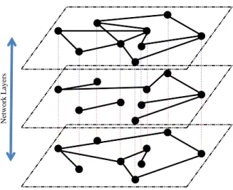
The other generalization in GEMF concerns the topology. In most epidemic models, the interaction among the agents is represented by the contact network. However, as discussed in Section II-C, the types of the interaction can be different in a complex network. For our modeling purpose, we represent the topology bylayers of graphsG(N ), whereN is the set
of nodes, denoting the agents, andis the set of edges which
represents the interaction between each pair of individuals in the -th layer. These graphs have the same nodes but the edges can be different. The adjacency matrix corresponding to the graph G is denoted by A = []×. If agent can
influenceagentin the layer,= 1otherwise = 0. In
Network Lay
ers
Fig. 3. Network layers describe the different types of interactions among agents in GEMF. The vertical dotted lines emphasize that all graphs have same nodes but the edges are different.
our model. A representation of the network layering structure is depicted in Fig. 3.
IV. AGENT-LEVELDESCRIPTION OF THEMARKOV SPREADINGPROCESS
The network state()follows a continuous-time Markov process. Knowing that the network is in state () at time , what is the network state (+∆) at time +∆? In a network of interacting agents, this question can be very complicated. Instead, a more natural approach is to describe the agent state(+∆)given the network state()at time
. The spreading process is fully described if the probability to record a transition from compartment to compartment for agent , conditioned on the network state (), is known for all possible values of ,, and. In this section, we focus on deducing an expression for Pr[(+∆) =
|() = ()], which will be used later on to develop
the GEMF model. The challenge in deducing an expression forPr[(+∆) =|() = ()]is that there are too
many possibilities for the dependence of the transition→ of the individual agent on the network state. Here are a few examples: − the transition → happens completely independently from the states of other agents,−the transition →happens if the number of other agents in compartment are more than the number of agents in compartment,− the transition → happens if agents 1and2 are both in compartmentand the rate of the transition is the logarithm of the number of agents in compartment . All of these examples are legitimate so far. However, we need to specify the transition possibilities properly to develop a coherent and consistent epidemic spreading model.
A. Epidemic Spreading Process Modeling
The SIS N-Intertwined model [12] gives very good insights in how to properly define the transition possibilities to describe an epidemic spreading process. In the SIS model, there are two transitions. The curing process, which is basically the
transition from ‘infected’ state to ‘susceptible’, occurs inde-pendently from the states of other agents. Instead, the infection process, which refers to transition from ‘susceptible’ state to ‘infected’ state, happens through a different mechanism. A susceptible agent is in contact with some other agents. During the time interval( +∆], the susceptible agent receives the infection from its infected neighbor with some probability. The process of receiving the infection from one infected neighbor is independent from the process of receiving the infection from another neighbor. All the infected neighbors compete to infect the susceptible agent. The susceptible agent becomes infected when one of the neighbors succeeds to transmit the infection. The transitions in the SIS epidemic model are very similar to the transitions in most existing epidemic models. As a result, we impose a similar structure of independent competing processes to the generalized spreading model.
Assumption 1: A transition → for agent is the result of several statistically independent competing processes: the process → for agent that happens independently of the states of other agents, and the process → for agent because of interaction with agent 6= , for each ∈{1 }\{}.
According to Assumption (1), the interaction of agent with agent 6= is statistically independent of its interaction with agent ∈ { }. Define the auxiliary counting process →
() () corresponding to the interaction of agent with agent. For convenience of notations, let(→)()correspond to the transition for agentoccurring independently from the states of other agents. According to Assumption 1, conditioned on the network state, these counting processes are statistically independent. The transition→occurs in the time interval ( +∆]if any of these counting processes record an event. Therefore, Pr[(+∆) = |() = ()] can be
written as
Pr[(+∆) =|() = ()] =
Pr[∃∈{1 }s.t.(→)(+∆)−(→)()6= 0|()] (4) Each of the counting processes →
() () is a Poisson process with the rate(→)(), to be determined. Therefore, Pr[(→)(+∆)−(→)()6= 0|()] =(→)()∆+(∆)
(5) The sum of independent Poisson processes is also a Poisson process with aggregate rate equal to the sum of the individual rates (see Th. 7.3.4 in [16]). Therefore,
Pr[(+∆) =|() = ()] = ∆ X =1 (→)() +(∆) (6) The remaining part of this section is dedicated to properly find(→)().
1) Nodal Transition: As discussed earlier, anodaltransition occurs independently from the states of other agents. For example, in the SIS model, the curing process is the result of a nodal transition. The curing process happens with rate
regardless of the infection status of other agents. In general, for the nodal transition→, we can consider a rate1
≥0,
which is actually the rate for the counting process →
() (), i.e.,
(→)() = (7)
2) Edge-Based Transition: The edge-based transitions are different from nodal transitions because they depend on the states of other agents. For example, in the SIS model, the infection process is an edge-based transition. The susceptible agent becomes infected with rate if it is in contact with infected agent . In the SIS model, the existence of contact among agents is determined by the contact network. However, we extend the concept of contact network to multi-layer networks. In our formulation, the interactions among agents are not limited to contacts. For example, agents might also exchange information. Corresponding to each layer , there is one influencer compartment. It is possible that the
influencer compartment of two distinct layers is the same. For example, recall the extended SAIS model with three network layers proposed in Section II-C. For the contact network and the infection information dissemination network, ‘infected’ is the influencer compartment. While for the alert information dissemination network, ‘alert’ is the influencer compartment. The transition from compartment to is characterized by the transition rate≥0for layer. In general, the edge-based transition from to 6= through edge ( ) is described by (→)() = X =1 1{()=} (8) where1{·}is the indicator function.
A transition→occurs if a neighbor , i.e.,= 1,
is in. Assigning only one influencer compartment to a graph
layer allows the elegant development of the subsequent anal-ysis. However, a more general possibility is that a transition → occurs if a neighbor , i.e., = 1, is in a subset
of the compartments, say1 or2. This case can be treated
within the same structure of GEMF. In this case, we can count the network layer twice. Therefore, we assume that the first time the graph has the influencer compartment 1 and the second time the graph has the influencer compartment 2. An example of this case is shown in Section VI-D.
B. Transition Rate Graphs
In order to make the subsequent developments systematic, we propose to use transition rate graphs defined as follows. A nodal transition rate graph is graph with nodes where each node represents a compartment. A directed link ( ) from torepresents the nodal transition→weighted by the positive transition rate0. Corresponding to the
nodal transition rate graph, the adjacency matrices of the nodal transition rates is defined as
,[]× (9)
1Here
is a non-negative scalar which represents nodal transitions. It should not be confused with the Kronecker delta symbol.
I S Ϯ ϭ δ I S Ϯ ϭ β
a)
b)
Fig. 4. Transition rate graphs in the SIS model: a) nodal transition rate graph; nodes represent the two compartments ‘susceptible’ and ‘infected’, directed link fromtorepresents curing process (a nodal transition) weighted by the curing rate 0, and b) edge-based transition graph of the contact network layerG; directed link fromtorepresents the infection process (edge-based transition) weighted by the infection rate 0. For the contact network, the influencer compartment is1= 2, i.e., ‘infected’.
S I A S I A δ κ β βa
a)
ϯb)
Ϯ ϭ ϯ Ϯ ϭFig. 5. Transition rate graphs in the SAIS model: a) nodal transition rate graph; nodes represent the three compartments ‘susceptible’, ‘infected’, and ‘alert’, directed link fromtorepresents curing process (a nodal transition) weighted by the curing rate 0, and b) edge-based transition graph of the contact network layerG; directed link fromtorepresents the infection process (edge-based transition) weighted by the infection rate 0, directed link from to represents the alerting process (edge-based transition) weighted by the alerting rate 0, directed link fromto represents the alerted infection process (edge-based transition) weighted by the alerted infection rate0. For the contact network, the influencer compartment is1= 2, i.e., ‘infected’.
An edge-based transition rate graph, corresponding to the network layerGis a graph with nodes where each node
represents a compartment. A directed link( )fromto represents the edge-based transition →weighted by the positive transition rate rate0in network layer with influencer compartment . Corresponding to the edge-based
transition rate graph, the adjacency matrices of the edge-based transition rates is defined as
,[]× (10) For example, in both SIS and SAIS model described in Section II-A and Section II-B, only the curing process is a nodal transition. The nodal transition rate graphs for the SIS and SAIS models are shown in Fig. 4 and Fig. 5, respectively. The schematics of the nodal transition rate graph in general is drawn in left hand side of Fig. 6. In both SIS and SAIS models described in Section II-A and Section II-B, respectively, the contact network is the only network layer. Therefore, these two models have one based transition rate graph. The edge-based transition rate graphs for the SIS and SAIS models are shown in Fig. 4 and Fig. 5, respectively. The schematics of the transition rate graphs in general is drawn in Fig. 6.
In Section V (see (27), below), the Laplacian (see, [28]) matrices associated to the transition rate graphs appears in the expression of GEMS.
3 5 1 4 2 6 3 5 1 4 2 6 δ51 δ24 δ26 βl,51 βl,36 βl,32 βl,43
a)
b)
Fig. 6. Transition rate graphs in GEMF: a) nodal transition rate graph; nodes represent compartments, directed link( )represent nodal transition
→weighted by the transition rate0, and b) edge-based transition graph of network layer G; directed link ( )represent the edge-based transition →weighted by the transition rate 0in network layer. The inducer compartment of layeris.
C. Agent-Level Markov Description of the Spreading Process In Section IV-A, we developed the expressions for the nodal transition and edge-based transitions. Substituting (7) and (8) into (6) yields
Pr[(+∆) =|() = ()] =
∆+∆
X
=1() +(∆) (11) for ={1 }and6=, where
(),
X
=1
1{()=} (12)
is the number of neighbors of agent in G that are in the
corresponding influencer compartment.
Equation (11) provides an agent-level description of the Markov process. It can directly be used for Monte Carlo numerical simulation of the spreading process.
V. GEMF: GENERALIZEDEPIDEMICMEAN-FIELD MODEL
The objective of this section is to derive the time evolution of the state occupancy probabilities.
A. Exact Markov Differential Equation
In the previous section, the spreading model was described and the corresponding Markov process was derived in (11). The evolution of the state occupancy probabilities, associated to a Markov process, follows a set of differential equations known as the Kolmogorov differential equations. The deriva-tion of the Kolmogorov differential equaderiva-tion of a Markov process is fairly standard (see, [16], [29]) when the transition rates between the states of the Markov process are known. However, the challenge here is that the network states are the actual Markov states and instead of the transition rates between the network states, we have the agent-level description of the transitions in (11). In this section, we derive the differential equations directly from (11).
According to (11), the probability of remaining in the previous state is
Pr[(+∆) =|() = ()] =
1− X
6=
Pr[(+∆) =|() = ()] (13)
Combining (2), (11), and (13) leads to [(+∆)|() = ()] = ⎡ ⎢ ⎢ ⎢ ⎢ ⎢ ⎢ ⎢ ⎢ ⎢ ⎢ ⎢ ⎣ 1+P=11() .. . (−1)+P=1(−1)() −˜−P=1˜() (+1)+P=1(+1)() .. . +P=1() ⎤ ⎥ ⎥ ⎥ ⎥ ⎥ ⎥ ⎥ ⎥ ⎥ ⎥ ⎥ ⎦ ∆++(∆) (14) where ˜ , X 6= ˜, X 6= (15)
and(∆)is a function of higher order terms of∆satisfying the condition
(∆) = 0 (16) where is the all ones vector with appropriate dimensions.
Define the generalized transition matrices ∈R× and
∈R
× with the elements
(),−
¡
¢
,− (17)
According to definitions (15) and (17), the matrices and
are actually the Laplacian matrices of transition rate graphs, defined in Section IV-B.
Using (14) and the definition (17), [(+∆)|()] is
obtained as [(+∆)|()] = −()∆ − X =1 ()()∆ +() +(∆) (18)
where()is defined in (12). Computing the expected value
of each side of (18), we get
[(+∆)] = −[()]∆ − X =1 [()()]∆ +[()] + ¯(∆) (19)
where¯(∆) =[(∆)]and the formula for iterative expec-tation (see [30]) rule [[|]] = [] has been used to
find [(+∆)]. Moving the [()] term in (19) to the
left side and dividing both sides by∆ yields [(+∆)]−[()] ∆ = −[()]− X =1 [()()] + 1 ∆¯(∆) (20) Letting ∆→0in (20), we obtain [()] =− [()]− X =1 [()()] (21) Using (12), the term [()()]in (21) can be written
as [()()] = X =1 [()()] (22) The term [()()] is actually embedded in [()⊗ ()]. Therefore, the evolution of [()] depends on
[()⊗()] term, which is the joint state of pairs of
nodes. This means that the marginal information about the compartmental occupancy probabilities is not enough to fully describe the time evolutions of the probabilities. If we continue to derive the evolution law for [()⊗()], it turns out
that the time derivative of[()⊗()]depends on terms of
the form [()⊗()⊗()], which are the joint states
of triplets. This dependency of the evolution of expectation of -node groups on expectation of (+ 1)-node groups continues until reaches to=. As a result, any system describing the evolution of the expected value of the joint state of any group of nodes is not a closed system. When =, the expectation of the joint state of all nodes [1()⊗· · ·⊗()], which according to definition (3)
is actually the expectation of the network state, satisfies a differential equation of the form
[] =−Q [] (23) whereQ∈R ×
is the infinitesimal generator (see [16], [29]) of the underlying Markov process. The Kolmogorov differential equation (23) is, which we refer to as the exact Markov model, is derived explicitly in the Appendix.
The exact Markov equation (23) fully describes the system. However, the above differential equation has states.
Therefore for large values of, it is neither analytically nor computationally tractable. In the following section, it is shown that through a mean-field type approximation, a differential equation with states can be derived.
B. GEMF: Generalized Epidemic Mean-Field Model
One way to reduce the state space size is to use clo-sure approximation techniques. As explained in the previous section, expectations of order depend on expectation of order+ 1. The goal of closure techniques is toapproximate the expectations of order + 1, and express them in terms of expectations of order less or equal to . In this way, a new set of differential equations is obtained which is closed
and has the state space size¡
¢
, which is polynomially growing by. The simplest approximation is the mean-field type approximation [31]. In first order mean-field models [12], the states of nodes are assumed to be independent random variables. It is also possible to consider higher order mean-field approximations. Cator and Van Mieghem [32] used a second order mean-field approximation and found more accurate performance of the model. Another approach is called themoment closuretechnique, where the joint states of triplets are assumed to have a specific distribution (usually normal or lognormal) [11], [31]. In this way the joint expectation of triplets are expressed in terms of expectations of pairs. Taylor et al. [31] have conducted a comparison of the performances of different approximations. In this paper, we use a fist order mean-field type approximation.
Using a first order mean-field type approximation, the joint expected values are approximated in terms of marginal expected values. Specifically, the term[()()]in (22) is approximated by
[()()]'([()])[()] (24) This approximation assumes independence between the ran-dom variables. Using the approximation (24), we can describe the time evolution of the expected values through a set of ordinary differential equations with states.
Denote by(), the expected value of at time, i.e.,
(),[()] (25)
Substituting [()()] = P=1(())() in (21), from (22) and (24), yields
() =− ()− X =1 X =1 (())() (26)
Arranging the terms in (26) specifies our generalized epidemic spreading model GEMF:
=− − X =1 ( X =1 ) ={1 } (27) Having initially
(0) = 1, the sum of the probabilities is guaranteed to be1at any time. The reason is that from (27)
does not change over time because
= −− X =1 ( X =1 ) = −()− X =1 ( X =1 )() = 0 (28)
The last conclusion is for the fact that= 0and= 0, since indeed and are the graph Laplacians for which is the eigenvector corresponding to a zero eigenvalue.
GEMF has a systematic procedure to develop different spreading mean-field models. For any specific spreading sce-nario, the compartment set, the network layers, and their
corresponding influencer compartments should be identified and the transition rate graphs should be drawn. The individual-based mean-field model of the spreading scenario is found by plugging the matricesand, obtained from the transition rate graphs, into GEMF (27).
C. Capabilities and Limitations of GEMF
GEMF can be used to describe a wide range of spreading scenarios in a systematic way. In GEMF, there is no approx-imation of the underlying networks. The only approxapprox-imation belongs to the mean-field-type approximation (24). How much this approximation results in deviation from exactness is a problem to be investigated and is out of the scope of this paper. The available studies for the mean-field SIS model (see, [33], [34]) can shed some light on this problem. Concerning the SIS model, extensive numerical simulations have shown that for sparser graphs the mean-field model is less accurate, while for graphs with more mixing, the mean-field model is more close to the exact process. For a homogeneous mixing contact network, it has been proved that the mean-field model is asymptotically exact, i.e., as → ∞. Furthermore, the accuracy of the mean-field model very much depends on the range of the epidemic parameters. For example, in the SIS spreading process, the mean-field model is accurate for large values of the infection rate for any graph. While for infection rates close to the epidemic threshold, there is considerable difference between the response of the mean-field model and the exact model. Additionally, it has been shown that mean-field SIS models fail to explain the existence of a stable disease-free absorbing state [35].
If the initial states are seeded according to an uncorrected distribution, i.e., at the initial time equation (24) is actually exact, then the mean-field model performs fairly accurately during the early stages of the system response. The reason for this is that nodes are poorly correlated at the early stage but become more and more correlated as time goes on. Accuracy of the transient response of mean-field models have been reported in [36] for the SIS spreading process. The steady state solution of the mean-field models are also important. For example, the steady state solution of SIS model belongs to the metastable state in SIS epidemic process [12]. If accuracy is of greater concern, then higher order closure techniques can be used. However, this will result in a much larger state space size. GEMF has the smallest state space size to describe the spreading process of the type considered in this paper. Any further reduction of the state space implies essentially adopting approximation on the network structure.
One of the great benefits of GEMF model is its analyt-ical tractability. Using SIS mean field model, the epidemic threshold was found to be the inverse of the spectral radius of the contact network. Finding relationships between spectral properties of underlying network layers and the spreading process is a problem of great interest. In particular, optimal design of some network layers given other network layers is very important from a technological view point. For example, Sahneh and Scoglio [37] used a mean-field SAIS model to find optimal topology of the information dissemination network given a contact network to reduce the impact of an epidemic.
VI. CASESTUDIES
In this section, we show that GEMF can reproduce the N-Intertwined SIS model [12] and the SIR model [14]. Further-more, an SAIS model with information dissemination and a model for a scenario where two pathogens are spreading in a host population are developed.
A. SIS N-Intertwined Model
The SIS N-Intertwined model [12] was explained in Section II-A. The number of compartments in this model is = 2. The epidemic parameters are the infection rate and the curing rate . In this model, the interaction is only through the contact graph. For the contact graph, ‘infected’ is the influencer compartment. Hence, = 1 and 1 = 2. The transition rate graphs for the SIS model are shown in Fig. 4. The adjacency matrices corresponding to the nodal and edge-based transition rate graphs follow from Fig. 4,
= ∙ 0 0 0 ¸ = ∙ 0 0 0 ¸ (29) Based on the GEMF (27), the compartment occupancy probability vectors satisfy the following differential equation
=− − X =12 (30)
for∈{1 }, where theandmatrices,
correspond-ing to and respectively, are
= ∙ 0 0 − ¸ = ∙ − 0 0 ¸ (31) Denote the probabilities of being susceptible by and
being infected by , i.e., = [ ]. Therefore, the
evolution of these probabilities can be described as
∙˙ ˙ ¸ = − ∙ 0 0 − ¸∙ ¸ −( X =1 ) ∙ − 0 0 ¸∙ ¸ = ∙ −(P=1) −+(P=1) ¸ (32)
Since,+= 1, the differential equation
=−+(1−)(
X
=1) (33) is obtained forand∈{1 }, which are the governing
equations for the N-Intertwined model in [12]. B. SIR N-Intertwined Model
Youssef and Scoglio [14] developed the SIR N-Intertwined model where each agent can be either ‘susceptible’, ‘infected’ or ‘recovered’. Therefore, the number of compartments in this model is = 3. A susceptible agent can become infected if it is surrounded by infected agents. The infection process is characterized by the infection rate. Furthermore, an ‘infected’ agent becomes ‘recovered’ with rate . Unlike the SIS model, a recovered agent does not become infected again in SIR model. Similar to SIS, there is only= 1contact
I S Ϯ ϭ δ I S Ϯ ϭ β R ϯ R R ϯ
a)
b)
Fig. 7. Transition rate graphs in the SIR model: a) nodal transition rate graph; nodes represent the two compartments ‘susceptible’, ‘infected’, and ‘recovered’, directed link from to represents curing process (a nodal transition) weighted by the curing rate 0, and b) edge-based transition graph of the contact network layerG; directed link fromtorepresents the infection process (edge-based transition) weighted by the infection rate
0. For the contact network, the influencer compartment is1= 2, i.e.,
‘infected’.
graph and 1 = 2. The transition rate graphs, shown in Fig. 7, illustrate that = ⎡ ⎣00 00 0 0 0 0 ⎤ ⎦ = ⎡ ⎣00 0 00 0 0 0 ⎤ ⎦ (34)
According to GEMF (27), the compartment occupancy probability vector satisfies the following differential equation
=− − X =12 (35)
for ∈{1 }, where the matrices are = ⎡ ⎣00 0 −0 0 0 0 ⎤ ⎦ = ⎡ ⎣0 −0 00 0 0 0 ⎤ ⎦ (36) based on (34).
Denote the probabilities of being susceptible, infected, and recovered by and , respectively, i.e., =
[ ]. The evolution of these probabilities can be
de-scribed as ⎡ ⎣ ˙ ˙ ˙ ⎤ ⎦ = − ⎡ ⎣00 0 −0 0 0 0 ⎤ ⎦ ⎡ ⎣ ⎤ ⎦ −( X =1 ) ⎡ ⎣0 −0 00 0 0 0 ⎤ ⎦ ⎡ ⎣ ⎤ ⎦ = ⎡ ⎢ ⎣ (P=1) −(P=1)− ⎤ ⎥ ⎦ (37)
Since, ++= 1, the differential equation
= −+(1−−)( X =1) = (38)
is obtained forandwhich is the SIR N-Intertwined model
in [14].
C. SAIS Model with Information Dissemination
Consider the SAIS model in Section II-C. Assume that a susceptible individual becomes alert not only if there are infected individual in its neighborhood, but also if there are alert individuals in the neighborhood. Assume that the latter happens with rate . The interaction is through the contact network, infection information dissemination network, and the alert information dissemination network. For both the contact network and the sensor network, ‘alert’ is the influencer compartment. For the information dissemination network, ‘alert’ is the influencer compartment. Hence,= 3 and1= 2,2= 2,3= 3. From Fig. 8, = ⎡ ⎣0 00 00 0 0 ⎤ ⎦ 1= ⎡ ⎣00 00 00 0 0 ⎤ ⎦ 2 = ⎡ ⎣00 00 0 0 0 0 ⎤ ⎦ 3= ⎡ ⎣00 00 0 0 0 0 ⎤ ⎦ (39)
From GEMF (27), the compartment occupancy probability vector satisfies the following differential equation
= − − X =1 121 (40) − X =1 222− X =1 233
for ∈{1 }, where thematrices are = ⎡ ⎣−0 0 00 − 0 ⎤ ⎦ 2 = ⎡ ⎣00 −00 00 0 − ⎤ ⎦ 2 = ⎡ ⎣0 00 −0 0 0 0 ⎤ ⎦ 3 = ⎡ ⎣0 00 −0 0 0 0 ⎤ ⎦ (41) according to (39).
A model very similar to (40), where there are only two layers of graphs, namely, the contact network and the infection information dissemination network, is used in [37] to assess the effectiveness of the information networks in reducing the impact of an epidemic. A novel information dissemination metric is introduced which measures the impact of information network on improving the resilience of the system against epidemic spreading. The developed information dissemination metric leads to a rigorous and elegant solution that determines the optimal topology of the information network to minimize the impact of an epidemic.
D. Multiple Interacting Pathogen Spreading
The problem of multiple pathogen spreading has recently attracted substantial attention (see e.g. [38]–[41]). Most mod-els consider a full cross immunity between pathogens, i.e., a node infected by one type of pathogen cannot be infected with any other type of pathogens at the same time. Beutel et al. [40] considered the case where the pathogens also have interacting
S I A ϭ Ϯ ϯ γ S I A ϭ Ϯ ϯ S I A ϭ Ϯ ϯ S I A ϭ Ϯ ϯ βa κ α δ c) d) a) b) β
Fig. 8. Transition rate graphs in the SAIS model: a) nodal transition rate graph; nodes represent the three compartments ‘susceptible’, ‘infected’, and ‘alert’, directed link fromtorepresents curing process weighted by the curing rate 0, directed link from to represents the un-alerting process weighted by the un-alerting rate 0, and b) edge-based transition graph of the contact network layerG; directed link fromtorepresents the infection process (edge-based transition) weighted by the infection rate 0, directed link fromtorepresents the alerted infection process (edge-based transition) weighted by the alerted infection rate 0. For the contact network, the influencer compartment is1= 2, i.e., ‘infected’. c) edge-based
transition graph of the infection information dissemination network layer
G; directed link fromtorepresents the alerting process weighted by the alerting rate 0, For the infection information dissemination network, the influencer compartment is1= 2, i.e., ‘infected’. d) edge-based transition
graph of the alert information dissemination network layerG; directed link from to represents the alerting process weighted by the alerting rate 0, For the alert information dissemination network, the influencer compartment is1= 3, i.e., ‘alert’.
effect on each other. In the model introduced by Marceau et al. [41], each pathogen has a separate contact network. In the following, we apply GEMF to develop an individual-based bi-spreading SIS model for epidemic spreading of multiple interacting pathogens, very similar to [40], where each pathogen, as in [41], has a different contact network.
Consider a spreading scenario where two pathogensand are spreading among a host population. The contact network for virusisG, whilespreads throughG. The transition
rates for the pathogens depend on each other. For example, from pathogen spreading point of view, a susceptible individual has different infection rate if it is infected by versus being susceptible to . In general, we assume the transition rates are 0 1 0 1. 0 1 0 1. For example, if an individual is infected by but is not infected by , then it recovers by rate0. Where as, if it is
also infected by, diseasegets cured by rate1. Similar
arguments apply for other rate terms.
For this spreading scenario, = 4 compartments can be defined to model the problem. Agent is in compartment1if it is susceptible to both and. It is2if it is susceptible to but infected by. It is3if infected by and susceptible to . And finally, it is 4 if it is infected by both and. The nodal and edge-based transitions are shown in Fig. 9.
ϭ ϯ ϰ Ϯ δB0 δA0 δA1 δB1 ϭ ϯ ϰ Ϯ βB0 βB1 ϭ ϯ ϰ Ϯ βA0 βA1
a)
b)
c)
Fig. 9. Transition rate graphs in the bispreading SIS model: a) nodal transition rate graph; nodes represent the four compartments ‘SS’, ‘SI’, , ‘IS’, and ‘II’, directed links fromIS toSS and fromII toSI represents curing process for virus weighed with curing rates0 and 1, respectively and the directed links fromSI to SS and from II toIS represents curing process for virusweighted by the curing rates0 and 1, respectively, and b) edge-based transition graph of the
contact network layerGfor virus; directed link fromSStoISand fromSI toII represents infection process for virusweighed with infection rates0 and1, respectively. For the contact networkG, the influencer compartment is = 34, i.e.,IS andII. c) edge-based transition graph of the contact network layerG for virus; directed link fromSS toSI and fromIS toII represents infection process for virusweighed with infection rates0and1, respectively. For the
contact networkG, the influencer compartment is = 24, i.e.,SI andII.
It follows from Fig. 9,
= ⎡ ⎢ ⎢ ⎣ 0 0 0 0 0 0 0 0 0 0 0 0 0 1 1 0 ⎤ ⎥ ⎥ ⎦ = ⎡ ⎢ ⎢ ⎣ 0 0 0 0 0 0 0 1 0 0 0 0 0 0 0 0 ⎤ ⎥ ⎥ ⎦ = ⎡ ⎢ ⎢ ⎣ 0 0 0 0 0 0 0 0 0 0 0 1 0 0 0 0 ⎤ ⎥ ⎥ ⎦ (42)
Therefore, according to the GEMF model (27), the com-partment occupancy probability vector satisfies the following differential equation ˙ = −− X =1 (3+4) − X =1 (2+4) (43) for ∈{1 }, where thematrices are
= ⎡ ⎢ ⎢ ⎣ 0 0 0 0 −0 0 0 0 −0 0 0 0 0 −1 −1 1+1 ⎤ ⎥ ⎥ ⎦ = ⎡ ⎢ ⎢ ⎣ 0 0 −0 0 0 1 0 −1 0 0 0 0 0 0 0 0 ⎤ ⎥ ⎥ ⎦
= ⎡ ⎢ ⎢ ⎣ 0 −0 0 0 0 0 0 0 0 0 1 −1 0 0 0 0 ⎤ ⎥ ⎥ ⎦ (44) VII. CONCLUSION
Inspired by existing individual-based epidemic models, the generalized epidemic mean-field (GEMF) model is proposed. While using the same common assumptions of most of the existing individual-based epidemic models, GEMF is capable to model more complex scenarios with multiple compartment and multiple network layers. The set of differential equations that fully describes the time evolution of the compartment occupancy probabilities has equations. Even though the system is linear, it is both computationally and analytically intractable. Through a mean-field type approximation, a set of nonlinear differential equations is developed. The latter system, referred to as GEMF, has a simple structure. It is characterized by the Laplacian of the transition rate graphs and the elements of the adjacency matrices of the network layers. A systematic procedure for developing the model is proposed that culminates in the GEMF governing equations (27). GEMF model is rigorous, allows analytical tractability, and is simple to be adopted to many specific spreading processes, as shown in the several examples presented in this paper. We believe that the GEMF framework has the potential to allow the development of many different and novel individual-based epidemic models considering new compartments and multiple complex interaction structures.
REFERENCES
[1] J. Kephart and S. White, “Directed-graph epidemiological models of computer viruses,” inSociety Symposium on Research in Security and Privacy, may 1991, pp. 343–359.
[2] J. Kleinberg, “Computing: The wireless epidemic,”Nature, vol. 449, no. 7160, pp. 287–288, 2007.
[3] M. Meisel, V. Pappas, and L. Zhang, “A taxonomy of biologically inspired research in computer networking,”Computer Networks, vol. 54, no. 6, pp. 901–916, 2010.
[4] A. Barab´asi and Z. Oltvai, “Network biology: understanding the cell’s functional organization,” Nature Reviews Genetics, vol. 5, no. 2, pp. 101–113, 2004.
[5] C. Lindemann and A. Th¨ummler, “Performance analysis of the general packet radio service,”Computer Networks, vol. 41, no. 1, pp. 1–17, 2003.
[6] C. Riddalls, S. Bennett, and N. Tipi, “Modelling the dynamics of supply chains,”International Journal of Systems Science, vol. 31, no. 8, pp. 969–976, 2000.
[7] N. Bailey, The mathematical theory of infectious diseases and its applications. London, 1975.
[8] Y. Moreno, R. Pastor-Satorras, and A. Vespignani, “Epidemic outbreaks in complex heterogeneous networks,”The European Physical Journal B - Condensed Matter and Complex Systems, vol. 26, pp. 521–529, 2002. [9] R. Pastor-Satorras and A. Vespignani, “Epidemic dynamics and endemic states in complex networks,”Phys. Rev. E, vol. 63, no. 6, p. 066117, May 2001.
[10] Y. Wang, D. Chakrabarti, C. Wang, and C. Faloutsos, “Epidemic spreading in real networks: An eigenvalue viewpoint,”Proc. 22nd Int. Symp. Reliable Distributed Systems, pp. 25–34, 2003.
[11] M. Keeling and K. Eames, “Networks and epidemic models,”Journal of the Royal Society Interface, vol. 2, no. 4, pp. 295–307, 2005. [12] P. Van Mieghem, J. Omic, and R. Kooij, “Virus spread in networks,”
IEEE/ACM Transactions on Networking, vol. 17, no. 1, pp. 1–14, 2009. [13] A. Ganesh, L. Massoulie, and D. Towsley, “The effect of network topology on the spread of epidemics,” inProceedings IEEE INFOCOM, vol. 2, 2005, pp. 1455–1466.
[14] M. Youssef and C. Scoglio, “An individual-based approach to SIR epidemics in contact networks,” Journal of Theoretical Biology, vol. 283, no. 1, pp. 136–144, 2011.
[15] S. Karlin and H. Taylor, A second course in stochastic processes. Academic Pr, 1981.
[16] P. Van Mieghem,Performance analysis of communications networks and systems. Cambridge Univ Press, 2006.
[17] P. Erd˝os and A. R´enyi,On the evolution of random graphs. Akad. Kiad´o, 1960.
[18] A. Barab´asi and R. Albert, “Emergence of scaling in random networks,”
science, vol. 286, no. 5439, pp. 509–512, 1999.
[19] J. Doyle, D. Alderson, L. Li, S. Low, M. Roughan, S. Shalunov, R. Tanaka, and W. Willinger, “The robust yet fragile nature of the internet,”Proceedings of the National Academy of Sciences, vol. 102, no. 41, p. 14497, 2005.
[20] J. Shao, S. Buldyrev, S. Havlin, and H. Stanley, “Cascade of failures in coupled network systems with multiple support-dependence relations,”
Physical Review E, vol. 83, no. 3, p. 036116, 2011.
[21] C. D. Brummitt, R. M. D’Souza, and E. A. Leicht, “Suppressing cas-cades of load in interdependent networks,”Proceedings of the National Academy of Sciences, 2012.
[22] S. Funk and V. Jansen, “Interacting epidemics on overlay networks,”
Physical Review E, vol. 81, no. 3, p. 036118, 2010.
[23] M. Dickison, S. Havlin, and H. Stanley, “Epidemics on interconnected networks,”Physical Review E, vol. 85, no. 6, p. 066109, 2012. [24] A. Saumell-Mendiola, M. A. Serrano, and M. Bogu˜n´a, “Epidemic
spreading on interconnected networks,”Phys. Rev. E, vol. 86, p. 026106, Aug 2012.
[25] Y. Wang and G. Xiao, “Effects of interconnections on epidemics in network of networks,” in Wireless Communications, Networking and Mobile Computing (WiCOM), 2011 7th International Conference on, sept. 2011, pp. 1–4.
[26] F. Sahneh and C. Scoglio, “Epidemic spread in human networks,” in
Proceedings of IEEE Conference on Decision and Control, 2011. [27] W. Richoux and G. Verghese, “A generalized influence model for
networked stochastic automata,” IEEE Trans. on Systems, Man and Cybernetics, Part A: Systems and Humans, vol. 41, no. 1, pp. 10–23, 2011.
[28] P. Van Mieghem,Graph Spectra for Complex Networks. Cambridge Univ Pr, 2011.
[29] S. Ross,Stochastic processes. John Wiley & Sons New York, 1983, vol. 23.
[30] C. Gardiner,Handbook of stochastic methods: For physics, chemistry and the natural sciences. Berlin: Springer, 2004.
[31] M. Taylor, P. Simon, D. Green, T. House, and I. Kiss, “From markovian to pairwise epidemic models and the performance of moment closure approximations,”Journal of Mathematical Biology, pp. 1–22, 2011. [32] E. Cator and P. Van Mieghem, “Second-order mean-field
susceptible-infected-susceptible epidemic threshold,” Physical Review E, vol. 85, no. 5, p. 056111, 2012.
[33] S. C. Ferreira, C. Castellano, and R. Pastor-Satorras, “Epidemic thresh-olds of the susceptible-infected-susceptible model on networks: A com-parison of numerical and theoretical results,”arXiv:1206.6728v1, 2012. [34] C. Li, R. van de Bovenkamp, and P. V. Mieghem, “The sis mean-feld n-intertwined and pastor-satorras & vespignani approximation: a comparison,”Physical Review E, vol. 86, no. 2, p. 026116, 2012. [35] P. Van Mieghem, “The N-intertwined SIS epidemic network model,”
Computing, pp. 1–23, 2011.
[36] Z. Chen and C. Ji, “Spatial-temporal modeling of malware propagation in networks,”Neural Networks, IEEE Transactions on, vol. 16, no. 5, pp. 1291–1303, sept. 2005.
[37] F. Sahneh and C. Scoglio, “Optimal information dissemination in epidemic networks,” inProceedings of IEEE Conference on Decision and Control, 2012, to appear.
[38] M. Newman, “Threshold effects for two pathogens spreading on a network,”Physical review letters, vol. 95, no. 10, p. 108701, 2005. [39] M. Lipsitch, C. Colijn, T. Cohen, W. Hanage, and C. Fraser, “No
coexistence for free: neutral null models for multistrain pathogens,”
Epidemics, vol. 1, no. 1, p. 2, 2009.
[40] A. Beutel, B. Prakash, R. Rosenfeld, and C. Faloutsos, “Interacting viruses in networks: can both survive?” in Proceedings of the 18th ACM SIGKDD international conference on Knowledge discovery and data mining. ACM, 2012, pp. 426–434.
[41] V. Marceau, P. No¨el, L. H´ebert-Dufresne, A. Allard, and L. Dub´e, “Modeling the dynamical interaction between epidemics on overlay networks,”Physical Review E, vol. 84, no. 2, p. 026105, 2011.
APPENDIX
DERIVATION OFEXACTMARKOVEQUATION In this section, we explicitly derive the expression for Q
in (23). The idea is to derive the expression for [(+ ∆)] as a function of[()]. For this end, first we find the expression for the conditional expectation[(+∆)|()]. Then, the expression for [(+∆)]is found by averaging out the conditional. For small values of ∆, we can assume that only one transition happens at each time step, i.e., starting at network state at time , the network state can only go to a new state at time +∆for which only the state of a single node has been changed. Given the network state () =,
state () = of each agent are can be determined and we have
=1⊗· · ·⊗ (A.1) Since only at most one single node can make a transition, the conditional expected value of the network state at time+∆ is
[(+∆)|() =] =
X
=11⊗· · ·⊗
[(+∆)|() =]⊗· · ·⊗ (A.2) where from (18), the expression for[(+∆)|() =]
is [(+∆)|() = ] =−∆ − X =1 X =1 1{=} ∆ +() +(∆) (A.3) By averaging over all of the possible network states, the expected value of the network state at time+∆is found
[(+∆)] = X =1 [(+∆)|() =] Pr[() =] = X =1 (X =11⊗· · ·⊗ [(+∆)|() =]⊗· · ·⊗) Pr[() =] (A.4) Substituting for[(+∆)|() =]from (A.3),[(+
∆)]is deduced to be [(+∆)] =−Q[()]∆ − X =1 Q[()]∆+[()] +(∆) (A.5) where Q = X =1× ⊗· · ·⊗⊗· · ·⊗×
andQ is such that its−th column is col(Q ) = X =11⊗· · ·⊗ ( X =1 1{=})⊗· · ·⊗ (A.6) By letting∆→0in (A.5), the time evolution of[]can be fully described by [] =−Q [] (A.7) where Qis defined as Q=Q+ X =1 Q (A.8)
The differential equation (A.7) is referred to as the exact Markov equation.