MULTIPLE-INPUT MULTIPLE-OUTPUT WIRELESS SYSTEM DESIGNS WITH IMPERFECT CHANNEL KNOWLEDGE

(1)

MULTIPLE-INPUT MULTIPLE-OUTPUT WIRELESS SYSTEM

DESIGNS WITH IMPERFECT CHANNEL KNOWLEDGE

by

Minhua Ding

A thesis submitted to the

Department of Electrical and Computer Engineering in conformity with the requirements

for the degree of Doctor of Philosophy

Queen’s University Kingston, Ontario, Canada

July 2008

(2)

ABSTRACT

Employing multiple transmit and receive antennas for wireless transmissions opens up the opportunity to meet the demand of high-quality high-rate services envisioned for future wireless systems with minimum possible resources, e.g., spectrum, power and hardware.

Empowered by linear precoding and decoding, a spatially multiplexed multiple-input multiple-output (MIMO) system becomes a convenient framework to offer high data rate, diversity and interference management. While most of the current precoding/decoding de-signs have assumed perfect channel state information (CSI) at the receiver, and sometimes even at the transmitter, in this thesis we will design the precoder and decoder with imperfect CSI at both the transmit and the receive sides, and investigate the joint impact of channel estimation errors and channel correlation on system structure and performance. The mean-square error (MSE) related performance metrics will be used as the design criteria.

We begin with the minimum total MSE precoding/decoding design for a single-user MIMO system assuming imperfect CSI at both ends of the link. Here the CSI includes the channel estimate and channel correlation information. The closed-form optimum precoder and decoder are determined for the special case with no receive correlation. For the general case with correlation at both ends, the structures of the precoder and decoder are also determined. It is found that compared to the perfect CSI case, linear filters are added to the transceiver structure to balance the channel noise and the additional noise caused by imperfect channel estimation, which improve system robustness against imperfect CSI.

(3)

Furthermore, the effects of channel estimation error and channel correlation are coupled together, and are quantified by simulations.

With imperfect CSI at both ends, the exact capacity expression for a single-user MIMO channel is difficult to obtain. Instead, upper- and lower-bounds on capacity have been de-rived, and the lower-bound has been used for system design. The closed-form transmit co-variance matrix for the lower-bound has not been found in literature, which is referred to as the maximum mutual information design problem with imperfect CSI. Here we transform the transmitter design into a joint precoding/decoding design problem. The closed-form optimum transmit covariance matrix is then derived for the special case with no receive cor-relation, whereas for the general case with non-trivial correlation at both ends, the optimum structure of the transmit covariance matrix is determined. The close relationship between the maximum mutual information design and the minimum total MSE design is discovered assuming imperfect CSI. The tightness and accuracy of the capacity lower-bound is eval-uated by simulation. The impact of imperfect CSI on single-user MIMO ergodic channel capacity is also assessed.

For robust multiuser MIMO communications, minimum average sum MSE transceiver (precoder-decoder pairs) design problems are formulated for both the uplink and the down-link, assuming imperfect channel estimation and channel correlation at the base station (BS). We propose improved iterative algorithms based on the associated Karush-Kuhn-Tucker (KKT) conditions. Under the assumption of imperfect CSI, an uplink–downlink duality in average sum MSE is proved, which is often used to simplify the more involved downlink design. As an alternative for solving the uplink problem, a sequential semidefi-nite programming (SDP) method is proposed. Simulations are provided to corroborate the analysis and assess the impacts of channel estimation errors and channel correlation at the base station on both the uplink and the downlink system performances.

(4)

Acknowledgments

Foremost, I would like to thank my advisor, Prof. Steven D. Blostein, for his guidance, patience, and full support during the past five years. I am grateful to him for his encour-agement and patience, especially during the time I needed these most. I am constantly surprised by his technical intuition, and I hope I have learned a bit from him in the way of thinking and carrying out research.

I also want to thank the thesis committee members, Prof. Wei Yu from University of Toronto, Prof. Glen Takahara from Dept. of Mathematics and Statistics, Prof. Il-Min Kim, and Prof. Prof. Alois P. Freundorfer for their taking time to review my thesis.

The kind help received at the early stage of the thesis research from Prof. Norman Rice of Dept. of Mathematics and Statistics is deeply appreciated.

I would like to express sincere thanks to all my lab colleagues, past and present, with whom I have worked and shared my life. They are: Lucien Benacem, Yu Cao, Luis Gurrieri, Leon Lee, Guangping Li, Patrick Li, Hani Mehrpouyan, Wei Sheng, Constantin Siriteanu, Yi Song, Edmund Tam, Neng Wang, Jinsong Wu, and Yi Zheng. I want to thank Yu Cao for many helpful discussions with respect to my thesis, as well as for numerous lifts I received from him. My thanks go to Constantin Siriteanu for reviewing the thesis draft and for his encouragement over these years.

My life here has been an enjoyable journey due to all my friends and all the kind people I have met, at Queen’s or outside Queen’s. Their characters have enriched my own. In

(5)

particular, I want to thank Bei Cai from Dept. of Physics at Queen’s for her great friendship. Last, but not the least, I want to thank all my family members in China, my parents, my sister, and Weilong Qu, for their support.

(6)

List of Tables

3.1 An iterative algorithm for solving (3.9) in the general case . . . 36 4.1 An iterative algorithm for solving (4.8) [with the MSE matrix given by (3.8)] 73 5.1 The KKT-based iterative algorithm for solving (5.2) . . . 99 5.2 The KKT-based iterative algorithm for solving (5.4) . . . 99 5.3 The SDP-based iterative algorithm for solving (5.2) [the sequential SDP

method] . . . 104 5.4 Channel correlation exponents and estimation error variances (M=6) . . . 105 5.5 Channel correlation exponents and estimation error variances (M=8) . . . 106 5.6 A comparison of the two algorithms given in Tables 5.1 and 5.3 . . . 107

(11)

List of Figures

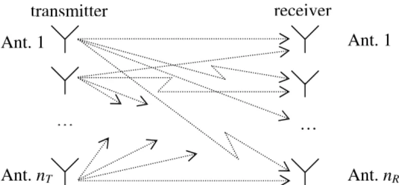
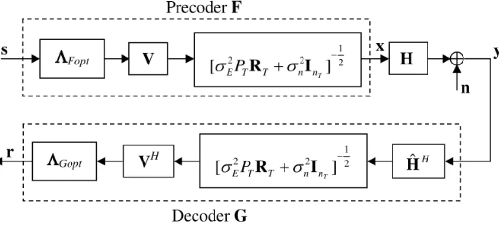
2.1 A single-user (point-to-point) wireless channel with multiple transmit and receive antennas. . . 11 2.2 A single-user (point-to-point) MIMO system with linear precoding/decoding. 16 2.3 Uplink and downlink MIMO transmissions with linear precoders/decoders . 21 3.1 Explicit structures of the optimum precoder and decoder. . . 32 3.2 Diagonalization of the equivalent channel (3.16). . . 33 3.3 The ABER from minimum total MSE design with perfect CSI. nT =nR=

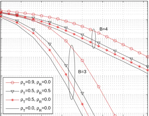
4, B = 3 or 4. Different amounts of channel correlation are considered:

ρT =0.0,0.5,0.9 andρR=0.0,0.5. . . 40

3.4 The ABER from minimum total MSE design with imperfect CSI. nT = nR=4, B = 3 or 4. Different amounts of channel correlation are considered. Ptr/σn2=26.016 dB. The values ofσce2 are 0.01, 0.015, and 0.0739, forρT

= 0.0, 0.5, and 0.9, respectively. Correspondingly, the values of σ_E2 are 0.0099, 0.0148, and 0.0689, forρT = 0.0, 0.5, and 0.9. . . 42

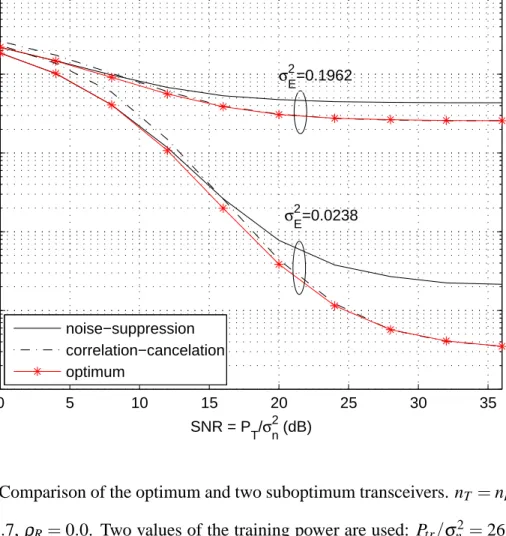
3.5 Comparison of the optimum and two suboptimum transceivers. nT =nR=

4, B = 3, ρT =0.7, ρR=0.0. Two values of the training power are used: Ptr/σn2=26.016 dB (corresponding toσE2 = 0.0238), and Ptr/σn2=16.016

(12)

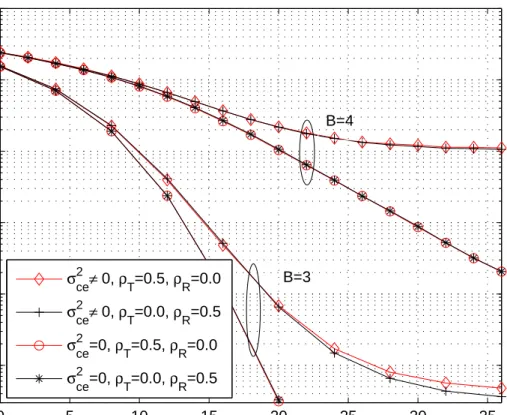
3.6 Effect of transmit correlation vs. effect of receive correlation. nT =nR=4, B = 3 or 4,(ρT,ρR)= (0.5, 0.0) or (0.0, 0.5), In the case of imperfect CSI, Ptr/σn2=26.016 dB. The values ofσce2 are 0.01 and 0.015, forρT = 0.0 and

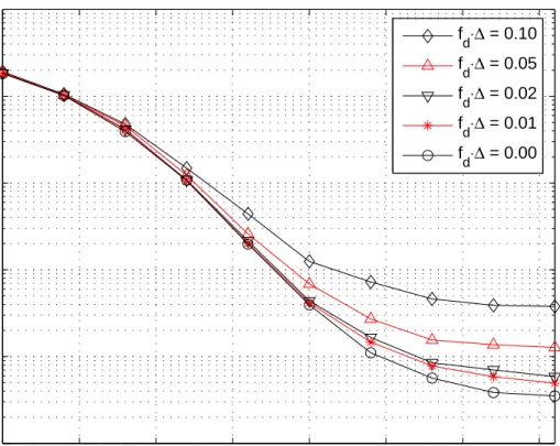
0.5, respectively. . . 46 3.7 The effect of feedback delay on system performance. nT =nR =4, B = 3,

ρT =0.7,ρR=0.0, Ptr/σn2=26.016 dB (corresponding toσE2= 0.0238). . 47

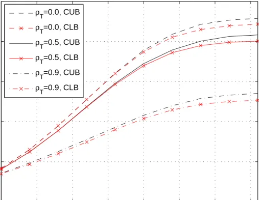
4.1 Comparison of the capacity upper- and lower-bounds. Both bounds are ob-tained using the optimum transmit covariance matrix for the lower-bound. nT =nR=4,ρR=0.0, Ptr/σn2=26.016 dB. The values ofσE2 are 0.0099,

0.0148, and 0.0689, forρT = 0.0, 0.5, and 0.9, respectively. . . 75

4.2 Ergodic capacity of a MIMO channel: optimum vs. uniform. nT =nR=4,

ρR=0.0. Perfect CSI at both ends is assumed for the optimum strategy. . . 77

4.3 Ergodic capacity lower-bound of a MIMO channel: optimum vs. uniform. nT =nR =4,ρR=0.0, Ptr/σn2=26.016 dB. The values ofσE2 are 0.0148

and 0.0689, forρT = 0.5 and 0.9, respectively. . . 78

4.4 Ergodic capacity of a MIMO channel. nT =nR=4. The two curves overlap

for(ρT,ρR) = (0.5,0.0)and(ρT,ρR) = (0.0,0.5). . . 79

4.5 Ergodic capacity lower-bound of a MIMO channel using the optimum trans-mit covariance matrix. nT =nR=4, Ptr/σn2=26.016 dB. The values ofσE2

are 0.0099, 0.0148, and 0.0689, forρT = 0.0, 0.5, and 0.9, respectively. The

two curves do not overlap for(ρT,ρR) = (0.5,0.0)and(ρT,ρR) = (0.0,0.5). 80

4.6 Ergodic capacity lower-bound of a MIMO channel: optimum vs. subopti-mum transmitters. nT =nR=4. ρT =0.7,ρR=0.0. Ptr/σn2=26.016 dB.

(13)

5.1 A comparison of the average sum MSEs obtained from the two algorithms in Tables 5.1 and 5.3. K =3, M =6, Ni =li =2, Ptr,i/σn2=30 dB, ∀i.

Channel correlation exponents and channel estimation error variances are given in Table 5.4. . . 109 5.2 A comparison between the average sum MSEs obtained from the

KKT-based algorithm and from solving a single SDP as described in Theorem 7. K =3, M =6, Ni=li=2; Ptr,i/σn2=29.66 dB, ρi=ρ =0.5, σEi2 =

˜

σ2

E =0.01,∀i. . . 110

5.3 Comparison of the ABERs of User 1 in the uplink with or without chan-nel estimation errors and with different amounts of chanchan-nel correlation. With imperfect CSI, the following parameters are used for this figure: M= 6,K=3,Ni=li=2. Ptr,i/σn2=30 dB,∀i. . . 111

5.4 Comparison of the ABERs of User 1 in the uplink with or without channel estimation errors and with different amounts of channel correlation. With imperfect CSI, the following parameters are used for this figure: K =3, M=6, Ni=li=2, Ptr,i/σn2=25 dB, i=1, . . . ,K. . . 113

5.5 Comparison of the ABERs of User 1 with channel estimation errors and different amounts of antenna diversity. K=3,Ni=li=2,Ptr,i/σn2=30 dB,

∀i. M =6 or 8. The corresponding correlation exponents and estimation error variances are given in Tables 5.4 and 5.5. . . 114 5.6 Duality in average sum MSE. K=3, M=6, Ni=li=2, i=1, . . . ,K. The

lowerρ0s are used:ρ1=0.5,ρ2=0.3,ρ3=0.2. Ptr,i/σn2=30 dB,∀i. . . . 115

5.7 Duality in average sum MSE. K=3, M=6, Ni=li=2, i=1, . . . ,K. The

(14)

5.8 Duality in individual users’ MSEs. K=3, M=6, Ni=li=2, Ptr,i/σn2=30

dB,∀i. The lowerρ0s are used: ρ1=0.5,ρ2=0.3,ρ3=0.2. For each user, curves for the uplink and the downlink overlap. . . 117 5.9 Comparison of the ABERs of User 1 in the downlink with or without

chan-nel estimation errors and with different amounts of chanchan-nel correlation. K =3, M =6, Ni=li=2,∀i. With imperfect CSI, Ptr,i/σn2=30 dB, ∀i.

The corresponding correlation exponents and estimation error variances are given in Table 5.4. . . 119 5.10 Comparison of the ABERs of User 1 in the downlink with or without

chan-nel estimation errors and with different amounts of chanchan-nel correlation. K=3, M=6, Ni=li=2,∀i. With imperfect CSI, Ptr,i/σn2=25 dB,∀i. . . 120

5.11 Comparison of the ABERs of User 1 in the uplink and in the downlink with or without channel estimation errors. K =3, M=6, Ni=li=2,∀i. With

imperfect CSI, Ptr,i/σn2 =30 dB, ∀i. The higher ρ0s are used: ρ1=0.8,

ρ2=0.7,ρ3=0.5. . . 121 5.12 Comparison of the ABERs of User 1 in the uplink and in the downlink with

or without channel estimation errors. K =3, M=6, Ni=li=2,∀i. With

imperfect CSI, Ptr,i/σn2 =30 dB, ∀i. The lower ρ0s are used: ρ1 =0.5,

(15)

Acronyms

ABER Average Bit Error Rate

AWGN Additive White Gaussian Noise

BC Broadcast Channel

BER Bit Error Rate

BLAST Bell Laboratories Layered Space-Time

BS Base Station

CCI Channel Correlation Information CDMA Code Division Multiple Access

CLB Capacity Lower-Bound

CMI Channel Mean Information

CSI Channel State Information

CSIR Channel State Information at Receiver CSIT Channel State Information at Transmitter

CUB Capacity Upper-Bound

DSL Digital Subscriber Line

EVD Eigenvalue Decomposition

i.i.d. independent and identically-distributed

KKT Karush-Kuhn-Tucker

(16)

LMMSE Linear Minimum Mean-Square Error

MAC Multiple Access Channel

MIMO Multiple-Input Multiple-Output

ML Maximum-Likelihood

MMSE Minimum Mean-Square Error

MS Mobile Station

MSE Mean-Square Error

MSMSE Minimum Sum Mean-Square Error

OSTBC Orthogonal Space-Time Block Code

QAM Quadrature Amplitude Modulation

QoS Quality of Service

SDP Semidefinite Programming (Program) SIC Successive Interference Cancelation SINR Signal-to-Interference-plus-Noise Ratio

SISO Single-Input Single-Output

SNR Signal-to-Noise Ratio

STBC Space-Time Block Code

STTC Space-Time Trellis Code

SVD Singular Value Decomposition

TDD Time-Division Duplex

(17)

List of Important Symbols

def

= Defined as

⊗ Kronecker product

(·)T _{Matrix or vector transpose}

(·)∗ Complex conjugate

(·)H _{Matrix or vector conjugate transpose (Hermitian)}

|x| Absolute value (modulus) of the scalar x det(·) Determinant of a matrix

log₂(·) Logarithm with base 2 ln(·) Natural logarithm

diag(x) Diagonal matrix with diagonal entries given by x E(·) Expectation of random variables

Im Identity matrix of size m×m

ℑ(·) Imaginary part of a complex-valued scalar, vector or matrix nT Number of transmit antennas in a single-user MIMO link nR Number of receive antennas in a single-user MIMO link ℜ(·) Real part of a complex-valued scalar, vector or matrix tr(·) Trace of a matrix

vec(·) Vectorization operator

(18)

min(a,b) Minimum of(a,b) max(a,b) Maximum of(a,b)

(a)+ max(a,0)

{ai}Ki=1 {a1,a2, . . . ,aK}

kxk Euclidean norm of a vector

AºB A−B is positive semidefinite, also denoted as B¹A AÂB A−B is positive definite, also denoted as B≺A

(19)

Chapter 1

Introduction

1.1

MIMO Systems for Future Wireless Communications

The goal of future wireless communications systems is to provide a wide variety of high-quality high-rate services with minimum requirements on spectrum, power consumption and hardware complexity. Toward this end, proper system structures as well as robust sys-tem designs are required to meet the challenges in wireless transmissions, such as multipath fading, limited spectrum resource, and interference. Recent research results have unveiled the multiple-input multiple-output (MIMO) system as a potential candidate to play a key role in future wireless [74].

A MIMO wireless system is commonly deployed by using multiple transmit and receive antennas. Early work on multi-antenna systems involves the use of antenna arrays at the receiver to provide spatial diversity against the random destructive effect of fading [9,42,78, 81]. There is a recent rich literature on employing multiple antennas at the transmitter and achieving diversity through space-time coding when there is no channel state information at the transmitter (CSIT) [2, 41, 99–101, 116], or through transmit beamforming when there is perfect CSIT [56]. Clearly, a MIMO system can be designed to fully exploit the transmit

(20)

and receive spatial diversity provided by the channel. The improvement in reliability of a MIMO system compared to that of a traditional single-input single-output (SISO) system is typically quantified by the diversity gain and the coding gain [53].

The use of multiple transmit and receive antennas also opens up the spatial domain for boosting data rate. While a flat-fading SISO Gaussian channel provides only a sin-gle narrow data pipe, a coherent MIMO channel can be represented as a set of parallel Gaussian channels and thus creates multiple data pipes for data transmission without addi-tional power or spectrum [26, 28, 29, 102], an appealing feature to cope with the scarcity

of wireless spectrum and the stringent power constraint on terminals. In particular, the er-godic (Shannon) capacity of a coherent MIMO channel scales linearly with the minimum of(nT,nR)[denoted as min(nT,nR)] in a rich-scattering spatially white environment, where nT and nRare the numbers of the transmit and receive antennas, respectively [29, 102]. The

gain in terms of ergodic capacity achieved by a coherent MIMO channel over that of a SISO channel is termed the spatial multiplexing gain [129], which can be reaped using the Bell Laboratories Layered Space-Time (BLAST) architecture [26, 27, 117].

Interestingly, MIMO spatial multiplexing systems harness the randomness of the chan-nel, whereas MIMO space-time coded systems combat it [104]. Although both spatial multiplexing and diversity gains can be simultaneously achieved by a MIMO system, there is a basic tradeoff between them [129].

For applications such as in wireless local area network (LAN) as well as in cellular communications, MIMO systems will likely be set up in a multiuser environment, where a multi-antenna base station (BS) simultaneously communicates with several multi-antenna mobile stations (MSs). There are two basic multiuser channels here. One is the multiple-access channel (MAC), also known as the uplink or the many-to-one channel [17, 24].

(21)

The other is the broadcast channel (BC), also referred to as the downlink or the one-to-many channel [16, 17]. Recent results from information-theoretic studies have completely characterized the capacity regions of the coherent Gaussian MIMO MAC [31, 54, 124] and BC [11, 107, 115, 123]. It has been found that in a multiuser environment, the use of multiple antennas introduces more flexibility to deal with the multiuser interference and enables simultaneous high-rate, multiuser communications, besides providing spatial multiplexing and diversity gains [104]. Similar to the single-user case, there is a tradeoff among the capabilities of spatial multiplexing, diversity and interference management in multiuser MIMO systems [105].

Thus, MIMO systems have been established as a promising transmission structure to achieve the goal of future wireless systems.

1.2

MIMO System Designs and Channel Knowledge

The promise of a high performance return from using MIMO systems largely relies on the assumption of perfect coherent reception, i.e., perfect channel state information at the receiver (CSIR), and even perfect CSIT with some designs.

In practice, however, perfect coherent reception (perfect CSIR) is unattainable due to channel estimation errors. Consequently, it is necessary to design a system robust to im-perfect CSIR.

Some popular MIMO systems, such as space-time coded systems and the BLAST ar-chitecture, have considered no CSIT, whereas others, e.g., transmit beamforming [3, 56] or generalized beamforming systems [85, 87, 120], have assumed perfect CSIT. Practical situations indicate that some forms of partial CSIT can be available [68, 109]. For exam-ple, partial CSIT can be acquired by transferring the CSIR to the transmitter via a feedback

(22)

link. Feedback is not an uncommon feature and it is present in most wireless systems, e.g., the power control channel in Code Division Multiple Access (CDMA) systems. If a system operates in the time-division duplex (TDD) mode, the transmitter can infer the CSI by measuring its received signal based on the reciprocity of wireless channels. CSIT obtained this way is usually imperfect due to channel estimation errors, erroneous CSIR, and/or limitation of the feedback link. However incomplete, CSIT, if efficiently used, can yield considerable performance gain in both space-time coded [44, 130, 131] and spatially-multiplexed systems [40], as opposed to the case of no CSIT. Therefore, intelligent MIMO systems designs must exploit the available CSIT.

The uncertainty in CSI can be modeled and dealt with in two different ways. One way is to model the error in channel knowledge as unknown but deterministic and bounded in a certain region. Worst-case optimizations are then employed to guarantee a (certain) minimum reliability level [33, 72, 111] [69, Chapter 7]. However, a worst-case design is rather conservative, since the worst case usually occurs with low probability [112]. Thus, an alternative way, which models the uncertainty by its first-order and second-order statistics [30, 31, 40, 44, 68, 109, 130, 131], is of particular interest and has been widely adopted. A design based on statistical channel information is called a stochastic robust design [69, Chapter 7].

As far as statistical uncertainty models are concerned, the channel mean information (CMI) and channel correlation information (CCI), obtained from channel estimation and propagation geometry measurement, respectively, are extensively used [31]. The CMI and CCI can be conveniently exploited using precoding or joint precoding and decoding. In particular, linear precoding/decoding is often preferred, due to the complexity constraint, especially for mobile terminals.

(23)

To make statistical CSI available at the transmitter, feedback is required, albeit infre-quent in slow-fading channels. If the feedback link is bandwidth-constrained, it will be more appropriate to employ limited-feedback designs [6, 55, 57, 58, 65, 118]. Nevertheless, the general stochastic robust designs usually lead to solutions that clearly describe sys-tem structures, and thus provide direct information on how impairments such as erroneous channel estimation and channel correlation affect system performance. The results from the general designs are also helpful in identifying key channel parameters that should be quantized and transferred back to the transmitter, as well as in assessing the performance of limited-feedback designs. Therefore, it is of great importance to study MIMO system designs with uncertain CSI modeled statistically.

1.3

Motivation and Thesis Overview

With proper linear precoder designs or joint linear precoder-decoder designs, a spatial mul-tiplexing system becomes a convenient framework to improve data rates, enhance link re-liability as well as offer a flexible diversity-multiplexing tradeoff for both single-user and multiuser MIMO communications. The joint precoder-decoder design is also known as (joint) transceiver optimization.

For single-user MIMO systems, various performance measures have been considered as the precoder design or joint design criteria, e.g., minimum total mean-square error (MSE) from all data streams [87, 120], minimum weighted MSE [85], maximum mutual information (capacity) [85, 87, 102], minimum Euclidean distance between received signal points [14], and minimum bit error rate (BER) [113, 119]. A comprehensive study of joint precoder-decoder designs under the MSE-based, the signal-to-interference-plus-noise-ratio (SINR)-based, or the BER-based criteria has been presented in [70].

(24)

Among the above performance measures, the MSE-related design criteria are of par-ticular interest to us. The minimum total MSE criterion aims at minimizing the trace of a MSE matrix, and balances interference and noise suppression. In addition, minimum sum MSE linear precoding and decoding designs have been applied to multiuser MIMO sys-tems [45, 91, 125]. The maximum mutual information design is also a MSE-related design, since it is equivalent to minimizing the determinant of the MSE matrix [87]. Although the minimum total (sum) MSE criterion does not account for the fairness among data streams (users), it generally leads to tractable analysis and overall good performance.

Most previous work on linear precoder designs or joint linear precoder and decoder de-signs for single-user MIMO spatial multiplexing systems has assumed perfect CSIR. Only a few studies have considered imperfect CSI at both ends, but these have not considered the effect of channel estimation error when coupled with channel transmit and/or receive correlation. Since these two impairments often coexist, it is important to investigate their joint impacts. Similar observations also apply to existing multiuser MIMO system designs. In this thesis, we will employ the spatial multiplexing framework with joint linear pre-coding and depre-coding for both single-user and multiuser communications in slow, Rayleigh flat-fading MIMO channels. We optimize the transceiver using the MSE-related design criteria. In the single-user case, the imperfect channel estimate as well as both transmit and receive correlation is assumed to be known to both ends of the link. In a multiuser scenario, we consider both channel estimation errors and channel correlation at the BS.

Note that the generic MIMO system model subsumes many other communication chan-nels, e.g., a bundle of twisted pairs in Digital Subscriber Line (DSL) or a frequency-selective channel with transmit and receive filterbanks [70, 80, 85, 86]. Therefore, by con-sidering narrow-band (flat-fading) channels does not necessarily limit our results for other channel conditions and system applications.

(25)

In Chapter 2, we briefly introduce basic MIMO communications in slow flat fading. The MIMO channel model used in this thesis is described. Single-user and multiuser MIMO systems with linear precoding and decoding are introduced here.

In Chapter 3, we study the joint linear precoding/decoding design to minimize total MSE from all data streams in a single-user MIMO system, under the assumption of imper-fect CSI at both ends. A detailed channel estimation method is introduced, which presents the specific CSI assumptions used thereafter. The minimum total MSE design is formu-lated as a non-convex optimization problem subject to a total transmit power constraint. The closed-form optimum precoder and decoder are derived for the special with no receive correlation. The optimum transceiver structure for the general case is also determined. Based on the optimum transceiver pair, we investigate the effects of channel estimation error and channel correlation on system structure and average BER performance.

In Chapter 4, we consider maximum mutual information design for a single-user MIMO system under the same CSI assumption as described in Chapter 3. With the assumed CSI, exact capacity expressions are difficult to determine. Instead, tight upper- and lower-bounds on the mutual information are employed for system design. While a capacity lower-bound has been formulated previously, the closed-form optimum transmit covariance matrix re-mains to be determined, subject to a total transmit power constraint. This is known as the maximum mutual information design, or the capacity lower-bound problem, in the case of imperfect CSI. We relate this problem to that of minimizing the log determinant of the MSE matrix, which is a non-convex problem. We then derive the structure of the opti-mum transmit covariance matrix by solving this new non-convex problem using the same methodology as in Chapter 3. Through this approach, the relationship between the mini-mum total MSE design and the maximini-mum mutual information design is also unveiled under the assumption of imperfect CSI. Using Monte Carlo simulations, we examine the tightness

(26)

of the ergodic capacity bounds and investigate the effects of channel estimation error and channel correlation.

Chapter 5 focuses on the joint linear precoder/decoder designs to minimize the sum MSE in multiuser MIMO systems. Both the uplink and the downlink are considered. Under similar CSI assumptions as in Chapter 3, we formulate the uplink and downlink minimum average sum MSE transceiver optimization problems. We extend and improve previous Karush-Kuhn-Tucker(KKT)-conditions-based algorithms so that they can be used in our case with reduced complexity. A duality in the average sum MSE between the uplink and the downlink is proved. For the uplink optimization, we also propose a sequential semidefinite programming (SDP) method. Based on optimized transceiver pairs, the effects of channel estimation errors and channel correlation at the BS are assessed.

Chapter 6 concludes this thesis and suggests future work.

1.4

Thesis Contributions

The primary contributions of this thesis are briefly summarized below:

• The minimum total MSE design is studied with imperfect CSI at both ends of a single-user MIMO link. Both channel estimation error and channel correlation are considered. Optimum structures of the linear precoder and decoder are derived. Our results gracefully fit those in the literature as channel estimation error diminishes. Based on analytical and simulation results, the impact of channel estimation error as well as the effect of transmit and receive correlation is assessed.

• When CSI is imperfect at both ends of a single-user MIMO link, the maximum mu-tual information design relies on a tight lower-bound on capacity. Previously, a nu-merical search method has been employed to find the optimum transmit covariance

(27)

matrix for this lower-bound. Here, the expression for the optimum transmit covari-ance matrix is determined by using a novel approach which solves an equivalent problem. The analytic solution clearly describes the transmitter structure. The accu-racy of using the optimum transmit covariance matrix is shown by comparing it with the uniform power allocation strategy. The effect of imperfect CSI on the ergodic capacity is also investigated.

• Under the imperfect CSI assumption, the relationship between the minimum total MSE design and the maximum mutual information design is discovered. Interest-ingly, analogous to the perfect CSI case, the two share the same transmitter struc-ture and differ mainly in power allocation with imperfect CSI. Alternatively, the two designs (under imperfect CSI) are connected through the minimum weighted MSE design. Therefore, our results provide a new perspective of the connection between two important quantities in estimation theory and information theory, i.e., the MSE from data estimation and the mutual information between channel input and output. • Minimum average sum MSE transceiver optimization problems are formulated for

multiuser MIMO uplink and downlink considering channel estimation errors and channel correlation at the BS. A duality in average sum MSEs for both links is proved theoretically. Unlike previous methods to prove duality, our method is solely based on the associated Karush-Kuhn-Tucker (KKT) conditions, and thus provides insight into the relation between the dual links. Improved KKT-conditions-based iterative algorithms are proposed for both links. For the uplink optimization, we also pro-pose a sequential SDP method. Effects of imperfect CSI are evaluated by computer simulations.

(28)

Chapter 2

Background

2.1

Single-user MIMO Communications over Flat-fading

Wireless Channels

2.1.1

MIMO Channel Model and System Model

Consider a wireless communication system with nT antennas at the transmitter and nR

antennas at the receiver (see Fig. 2.1) [53]. In a flat-fading channel, each signal path is represented by a random complex fading coefficient (channel gain) [78, 81], so that the MIMO channel in Fig. 2.1 is conveniently described by a matrix H, with its(j,i)-th element hj,idenoting the channel gain from transmit antenna i to receive antenna j, i=1, . . . ,nT,j=

1, . . . ,nR: H=       h1,1 . . . h1,nT . . . . . . . . . hnR,1 . . . hnR,nT      .

The random channel gains are modeled by circularly symmetric complex Gaussian random variables [78, 81], denoted as hj,i∼Nc(m_hj,i,1),∀i,j. If the mean of the channel gain (m_hj,i)

(29)

receiver transmitter Ant.nT Ant. 1 … … Ant. 1 Ant.nR

Figure 2.1. A single-user (point-to-point) wireless channel with multiple transmit and re-ceive antennas.

is non-zero, the channel is said to undergo Ricean fading. If m_hj,i=0, the channel undergoes Rayleigh fading. Note that the settings in this thesis are for Rayleigh fading channels.

A Rayleigh fading MIMO channel is said to be spatially white ifE(hj,ihn∗,m) =0,i,m=

1, . . . ,nT,j,n=1, . . . ,nR,i=6 m,j6=n, and is denoted by Hw. Here we have used E(·)to

denote the expectation of a random variable. Note that hwdef= vec(Hw)∼Nc(0,InR×nT),

where vec denotes the vectorization operation, and Im denotes the m×m identity matrix.

When there is spatial correlation, the following nonparametric channel model is commonly used [25, 95]: H=R 1 2 RHwR 1 2 T, (2.1)

where RT (nT×nT) and RR(nR×nR) denote the transmit and receive correlation matrices,

respectively. Thus [53], hdef=vec(H) = (R T 2 T ⊗R 1 2 R)hw∼Nc(0,R T T⊗RR), (2.2)

where ⊗ denotes Kronecker product, and the identity vec(ABC) = (CT ⊗A)vec(B) has been used [10, Table II, T2.13] (Note that this identity holds for complex matrices).

(30)

In practical downlink channels, the mobile is likely to be surrounded by a large number of local scatterers. The BS antennas, on the other hand, are often situated at high enough elevation to limit scattering and thus channels arising from the transmit antennas (in the downlink) are correlated. In this case,

H=HwR 1 2

T. (2.3)

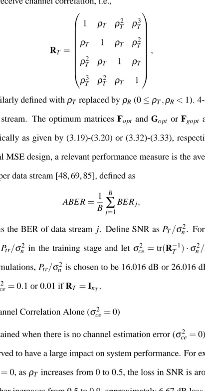
For an urban transmission environment, the exponential model has been proposed for transmit and receive correlation [12,30]. This means that the(j,i)-th element of RT is given

byρ_T|j−i|for i,j∈ {1, . . . ,nT}, whereρT represents the real-valued transmit correlation for

signals on adjacent antennas. The receive correlation matrix RR is similarly defined with

ρT replaced by ρR and with the indices ranging from 1 to nR. In subsequent chapters,

the exponential correlation model will be used for Monte Carlo simulations. However, it should be noted that our analytical results can be applied to any correlation model.

At a specific time slot, the received signal at antenna j is given by yj=

nT

∑

i=1

hj,ixi+nj,j=1, . . . ,nR,

or, in a vector form,

y=Hx+n, (2.4) where y= [y1, . . . ,ynR] T_{, n}_{= [}_n 1, . . . ,nnR] T _{and x}_{= [}_x 1, . . . ,xnT]

T _{are the received signal}

vector, the noise vector and the transmitter signal vector, respectively. The noise vector n is assumed to be spatially white and is distributed as n∼Nc(0,σ_n2·InR).

Further, consider the transmission of a nT ×N signal matrix composed of N data

vec-tors, X= [xt1, . . . ,_xtN]_{, over N consecutive time slots. In a slow-fading channel, it is often} assumed that the channel matrix is constant over a block of N time slots, i.e.,

(31)

Then,

Y=HX+N,

where Y and N denote the received signal matrix and the noise matrix, respectively, Y=

[yt1, . . . ,_ytN]_{and N}= [_nt1, . . . ,_ntN]_{. An equivalent vector signal model here is given by [53]} vec(Y) = (XT ⊗InR)h+vec(N).

2.1.2

Space-Time Coding for MIMO Systems

For slow-fading narrow-band transmissions, space-time coding is an important technique to extract the spatial diversity provided by the MIMO channel [2, 41, 99–101]. Block trans-mission is often assumed, as described in Subsection 2.1.1. Here X is referred to as the codeword matrix and is carefully designed with added redundancy. Two basic space-time codes, the space-time block code (STBC) and space-time trellis code (STTC), have been extensively studied. The orthogonal STBC (OSTBC) and the quasi-orthogonal STBC are two popular STBCs. In particular, the OSTBC is capable of providing full diversity gain

(nRnT)of the rich-scattering channel with low decoding complexity. Below is an example

of the OSTBC with nT =N=2 (also known as the Alamouti code [2]):

X=   x1 −x ∗ 2 x2 x∗₁   .

At each time slot, a column of the codeword matrix is transmitted across different antennas. At the end of a block, the receiver employs maximum-likelihood (ML) decoding to separate different transmitted symbols contained in a codeword.

In the design of a space-time code, several factors are considered: the diversity gain, the coding gain, the decoding complexity, the decoding delay (related to the block length N), and the symbol rate (defined as the ratio of the number of different symbols in a codeword and the block length N; 1 for the Alamouti code).

(32)

2.1.3

Spatial Multiplexing

In contrast to the space-time coded system, a spatially multiplexed system transmits differ-ent signal vectors across the transmit antennas at differdiffer-ent time slots, as described by (2.4). At the receiver, to minimize the error probability, ML detection should be employed. The problem with ML detection is its high complexity, which motivates the use of suboptimum detection schemes. Linear detection methods, such as the zero-forcing (ZF) and minimum MSE (MMSE), are widely used. The non-linear detectors, such as ZF detection with suc-cessive interference cancelation (ZF-SIC) and MMSE detection with SIC (MMSE-SIC), generally provide improved performance at the cost of increased complexity [53, 75].

2.1.4

Capacity of Coherent MIMO Channels in Flat Fading

Consider a Gaussian MIMO channel whose input-output relationship is given by (2.4). In coherent communications, the channel H is perfectly known at the receiver. Given H, the capacity is expressed as [102] C(H) =max p(x)I(x; y) = maxQº0 tr{Q}≤PT log₂det · InR+ 1 σ2 n HQHH ¸ (bits/channel use), where p(x)denotes the input distribution, I(·; ·)denotes the mutual information between channel input and channel output, PT is the total transmit power, and Q

def

= E(xxH) is the transmit signal covariance matrix. Qº0 means that Q is positive semidefinite. Here the transmitted signal vector is assumed to be zero-mean.

If the channel is unknown to the transmitter, uniform power allocation is used at the transmitter, i.e., Q= PT

nTInT, and

Cuni(H) =log2det

· InR+ PT nTσn2 HHH ¸ .

On the other hand, if the channel is perfectly known at the transmitter, the matrix channel can be decoupled into a set of parallel scalar Gaussian channels by means of singular value

(33)

decomposition (SVD) [37]. Specifically, let ˘r=rank(H) and let H be represented by its SVD:

H=U ˘˘ ΛΛΛ 1 2 _V˘H_,

where ˘U, ˘ΛΛΛand ˘V are nR×˘r, ˘r×˘r and nT ×˘r matrices, respectively. ˘ΛΛΛ=diag(λ˘1, . . . ,λ˘˘r) denotes a diagonal matrix composed of the non-zero eigenvalues of HHH arranged in de-creasing order. Then we have

˘ yi=        q ˘ λix˘i+n˘i, i=1, . . . ,˘r, ˘ ni, i= ˘r+1, . . . ,nR,

where ˘y=U˘Hy, ˘x=V˘Hx, and ˘n=U˘Hn. The transmit power is optimally allocated among the effective ˘r scalar channels using the well-known water-filling procedure [17, Chapter 10, pp. 250-253]. As a result [102],

˘

P_iopt= (µ˘ −σ_n2/λ˘i)+, i=1, . . . ,˘r,

where ˘µ is determined by ∑_i˘r₌₁P˘_iopt =PT, and (a)+ denotes max(a,0). The

capacity-achieving input distribution is giving by x∼Nc(0,Q˘), where

˘

Q=V˘·diag(P˘₁opt, . . . ,P˘_˘ropt)·V˘H

=_V˘_·₍_µ_˘_I_˘r₋_σ2

nΛΛΛ˘

−1

)+·V˘H, (2.5)

and the capacity is given by

Cw f(H) = ˘r

∑

i=1 log₂ " 1+( ˘ λiµ˘ −σn2)+ σ2 n # .

It is important to note that, due to CSIT, Cw f(H) is usually larger than Cuni(H),

es-pecially in the low to medium SNR region. For full-rank channels, Cuni(H) approaches Cw f(H)when PT goes to infinity.

(34)

channel Linear precoder F MIMO channel H Linear decoder G Noisen

r

s

CSIT CSIR

y

x

transmitter receiver

Figure 2.2. A single-user (point-to-point) MIMO system with linear precoding/decoding.

The ergodic capacity of a coherent MIMO fading channel is the capacity C(H)averaged over different channel realizations:

C=EH ½ max Q,tr(Q)≤PT log₂det · InR+ 1 σ2 n HQHH ¸¾ .

In [26,102], it has been shown that if H=Hw, then the capacity as expressed in this formula

scales linearly with min(nT,nR).

2.1.5

Exploiting CSIT Using Linear Precoding/Decoding in Coherent

Spatial Multiplexing

In traditional space-time coded or spatially multiplexed systems, no CSI is needed at the transmitter. However, an efficient use of the available CSIT is beneficial to system perfor-mance. A good example has been seen in Subsection 2.1.4, where CSIT is exploited to improve capacity. Through proper designs, it can also ameliorate error rate performance.

To account for CSIT, a simple and general framework employs linear precoding and decoding, as depicted in Fig. 2.2. The information symbols to be sent are denoted by a B×1 vector s, where the number of data streams, B (≤nT), is properly chosen and fixed.

(35)

channel realizations. The data vector is then fed into the precoder, denoted by F, which is a nT×B linear matrix processor and takes the available CSIT into account. In the literature, F

is sometimes referred to as a generalized beamformer or a prefilter. After the precoder, the data vector is transmitted across the slow-varying flat-fading MIMO channel H. The nR×1

received signal vector at the receive antennas is y=HFs+n, where n is the spatially and temporally white additive Gaussian noise with distributionNc(0,σn2·InR). In the receiver, a linear decoder described by the B×nR matrix G is employed to recover the original

information. The decoder can be interpreted as an equalizer. At the output of the decoder, the signal vector r is given by

r=Gy=G(HFs+n).

In some system structures, the decoder G does not appear, or equivalently, G is rep-resented by an identity matrix. For example, in Subsection 2.1.4, for the perfect CSIT case, F=Q˘ 12 [see (2.5)] and G is not needed. [Here the input s is an independent and identically-distributed (i.i.d.) Gaussian vector, distributed as s∼Nc(0,InT).]

The framework in Fig. 2.2 subsumes both space-time coded systems [44, 84, 130, 131] and spatially multiplexed systems [1,14,40,50,70,85,87]. With linear precoding/decoding, spatial multiplexing is not only capable of providing high data rate, but also capable of introducing redundancy (diversity) into the precoded data streams, as well as achieving a tradeoff between diversity and multiplexing. Therefore, throughout this thesis, we will concentrate on joint transceiver designs for spatially multiplexed systems.

As mentioned in Section 1.3, various design criteria have been considered, among which the MSE-related ones are most popular. Most of the existing MSE-related designs have assumed perfect CSIR, while the CSIT has been assumed to be perfect or partial. In Chapter 3 and Chapter 4, we will consider imperfect CSIR (i.e., non-ideal coherent recep-tion) and imperfect CSIT in the transceiver designs, and investigate the joint impact of

(36)

channel correlation and erroneous channel estimation on system structure as well as on error rate or data rate performance.

2.2

Multiuser MIMO Communications over Flat-fading

Wireless Channels

2.2.1

Multiuser MIMO Uplink and Downlink Systems in Flat Fading

Consider a single cell in a cellular communication system. The BS is equipped with M antennas. There are K users (mobile stations), each with Ni antennas, i=1, . . . ,K. The

uplink channels are denoted by Hi, i=1, . . . ,K, whereas the downlink channels are given

by HH_i , i=1, . . . ,K. (In Subsection 2.2.2, we will explain why the uplink and the downlink channels are denoted using the same set of symbols.)

2.2.1.1 The Uplink System Model

Let the(Nk×1)transmitted signal vector from the antennas of user k be denoted by xul,k, k=1, . . . ,K. The signal vector received at the BS antennas is a blend of those from different users contaminated by channel fading and noise, i.e.,

yul = K

∑

k=1

Hkxul,k+nul.

2.2.1.2 The Downlink System Model

In the downlink, the BS broadcasts a mixture of K (M×1)signal vectors, each intended for a different user. Different MSs receive different copies of the mixture which have gone through individual fading processes. For user j,

ydl,j=HHj " K

∑

k=1 xdl,k # +ndl,j, j=1, . . . ,K.

(37)

2.2.2

Multiuser MIMO Channels: Capacity Regions, Sum Capacities

and Duality

In multiuser communications, it is the simultaneously achievable performances for all users that interest us.

Given perfect knowledge of {Hk}Kk=1, the capacity region of a MIMO MAC has been reported in [31,54,124], which characterizes all the simultaneously achievable data rates of individual users. In particular, it has been shown that the sum capacity (i.e., the sum of data rates of all users) of a coherent Gaussian MIMO MAC grows linearly with min(M,∑K_k₌₁Nk)

[102].

In cellular systems, the demand of the downlink data transfer is expected to be several times greater than that of the uplink [4]. This makes the MIMO downlink transmission particularly important. On the other hand, it is often harder to find the optimum transmit strategy for the downlink [17, Chapter 14]. In fact, given perfect channel knowledge, the capacity region of a coherent Gaussian MIMO BC has only recently been determined in [115], where it is shown to coincide with the previously found dirty-paper coding (DPC) achievable rate region [11, 15, 31, 107, 123].

Interestingly, it has been proved in [107, 115] that the capacity regions of the Gaussian MIMO MAC and BC are identical under the same sum power constraint. Furthermore, if a specific set of transmit covariance matrices in MAC/BC achieve a certain set of data rates, then there exists another set of transmit covariance matrices in the BC/MAC that achieve the same set of rates. The explicit transformation between the two sets of covariance matrices is also described in [107]. This relationship between the MAC and the BC is known as the MAC-BC duality [107]. With duality, the capacity region of the MIMO BC can be computed more easily.

(38)

the optimum transmit strategy for the dual channel and then transform it back to the actual channel under investigation. No channel reciprocity is invoked. This explains the notation we have used for the MAC and BC channels in Subsection 2.2.1.

2.2.3

Linear Processing for Multiuser MIMO

Along with the discovery of capacity-achieving transmit strategies for multiuser MIMO, signal processing techniques have been proposed to approach the proposed capacity limits, e.g., Tomlinson-Harashima precoding and vector perturbation techniques for the downlink [36, 123]. In practice, we attempt to approach the limits using signal processing techniques that are easy to implement. As for single-user MIMO systems, linear signal processing plays an important role also for multiuser MIMO.

Various linear processing techniques have been proposed for multiuser MIMO systems, including those for both the uplink [43, 45, 91] and the downlink [13, 43, 47, 76, 89, 96, 103, 125].

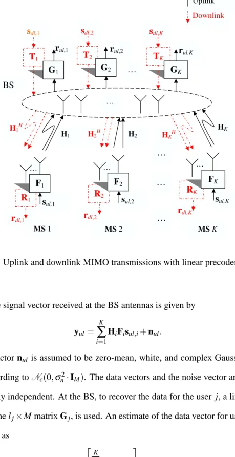
The minimum sum MSE (MSMSE) linear precoding/decoding design has been studied in [91] for the uplink, as well as in [47, 89, 103, 125] for the downlink, as a low-complexity and effective signal processing technique to manage both stream and multiuser inter-ferences and to provide high data rate and diversity. A schematic overview of multiuser MIMO systems with linear precoding/decoding is presented in Fig. 2.3.

2.2.3.1 The Uplink System Model with Linear Precoding/Decoding

Suppose that user i has lidata streams, denoted by the li×1 [li≤min(M,Ni)] vector sul,i, i=1, . . . ,K. These data vectors are assumed to be zero-mean, white[E(sul,isH_ul,i) =Ili,∀i], and mutually independent among users. Before the data streams are sent into the air, a linear precoder is employed for each user, which is denoted by the Ni×li matrix Fi, i=

(39)

r_dl_,1 MS₁ s_ul,2 s_dl_,2 s_dl_,_K H_K HK H H₁H H₂H H₁ MS₂ R₂ … … … … F₂ … … s_ul,1 sul,K r_ul,1 r_ul,2 _r ul,K BS T₁ G₁ T₂ G₂ T_K G_K R₁ R_K r_dl_,2 rdl,K F₁ FK MSK s_dl_,1 Uplink Downlink H₂ … …

Figure 2.3. Uplink and downlink MIMO transmissions with linear precoders/decoders

1, . . . ,K. The signal vector received at the BS antennas is given by yul =

K

∑

i=1

HiFisul,i+nul.

The noise vector nul is assumed to be zero-mean, white, and complex Gaussian, i.e.,

dis-tributed according toNc(0,σ_n2·IM). The data vectors and the noise vector are assumed to

be statistically independent. At the BS, to recover the data for the user j, a linear decoder, denoted by the lj×M matrix Gj, is used. An estimate of the data vector for user j can thus

be expressed as rul,j=Gj·yul =Gj " K

∑

i=1 HiFisul,i # +Gjnul, j=1, . . . ,K.

(40)

2.2.3.2 The Downlink System Model with Linear Precoding/Decoding

In the downlink, it is assumed that the data streams of user i are denoted by the li×1

vector sdl,i, and the linear precoder for user i at the BS is denoted by the M×limatrix Ti, i=1, . . . ,K. Similar to the uplink, the data vectors are assumed to be zero-mean and white [E(s_dl,isHdl,i) =Ili,∀i]. All data vectors are assumed to be mutually independent. The signal received at the antennas of user j is given by:

ydl,j=HHj " K

∑

i=1 Tisdl,i # +ndl,j, ∀j.

It is assumed that the noise vectors are mutually independent and ndl,j is distributed

ac-cording toNc(0,σn2·INj),∀j. Again, the data and the noise are assumed to be statistically independent. A linear decoder Rj (lj×Nj) is employed to recover sdl,j, which gives the

following estimate of sdl,j: rdl,j=Rj·ydl,j=RjHHj " K

∑

i=1 Tisdl,i # +Rj·ndl,j, j=1, . . . ,K.

2.2.3.3 Duality in Linear Precoding/Decoding designs for Multiuser MIMO Uplink and Downlink

Not surprisingly, an uplink–downlink duality also exists in the achievable MSE regions or the signal-to-interference-plus-noise ratio (SINR) regions of both links with linear precod-ing/decoding [89]. Perfect CSI and the same sum power constraint are assumed. Based on the duality, the more involved downlink minimum sum MSE linear precoding/decoding design has been tackled by forming and solving a dual uplink problem [89]. The same idea has also been adopted in [47].

In Chapter 5, we will further study the minimum sum MSE designs for both links and establish the duality in sum MSE with imperfect CSI.

(41)

Chapter 3

Minimum Total MSE Design with Imperfect CSI

at Both Ends

3.1

Introduction

Previously, the minimum total MSE transceiver designs for single-user MIMO systems have been studied with different assumptions of channel state information (CSI). In [70,85, 87,120], perfect channel state information at the transmitter (CSIT) as well as at the receiver (CSIR) is assumed. Later there have been more practical designs that consider imperfect CSIT. In [49], the minimum total MSE design has been studied with outdated CSIT and perfect CSIR. In [126, 127] [128, Section VII], it is assumed that the CSIT is the channel mean information (CMI) and/or the channel correlation information (CCI), whereas the receiver has perfect CSI. The more important case with imperfect CSIR has also been considered. For example, in [69, Chapter 7], the same imperfect CSI is assumed at both ends, but there the channel correlation has not been accounted for. In [128, Section VI], closed-form robust designs (including the minimum total MSE design) have been derived assuming that the same imperfect CSI, including channel mean and receive correlation information, is available to both ends. The same CSI assumption is also used in [92], where

(42)

the minimum total MSE design has been specifically studied. However, to the best of our knowledge, little attention has been paid to the joint design where the same imperfect CSI, including the channel mean and transmit correlation information, is available at both ends. This case is very interesting, since, as we have mentioned in Subsection 2.1.1 [see (2.3)], in practical downlink systems, the mobile is often surrounded by many local scatterers and channels from different antennas tend to be uncorrelated, whereas the channels from different BS antennas are often correlated due to limited scattering. The more general case, when there is channel estimation error and there is transmit and receive correlation, also remains as an open problem.

In this chapter, we address the problem of linear precoding/decoding to minimize the total MSE with imperfect CSI at both ends of a single-user MIMO link [18, 20]. The CSIR here is composed of the estimated channel (channel mean) as well as transmit (and more generally, transmit and receive) correlation information. To simplify the analysis, we assume the feedback is error-free and instantaneous, as in [66, 92, 121] [128, Section VI], which implies that the CSIT is the same as CSIR1. The assumption of instantaneous feedback is partly justified since, as will be shown by our simulations, the system maintains acceptable performance with a reasonably low feedback delay. The design under the above assumption is a step forward from that assuming perfect CSI at both ends [70, 85, 86, 120]. It can also serve as a basis for comparison to future system designs which explicitly take into account the errors and/or delays in the feedback link.

The basic system model used in this chapter has been introduced in Subsection 2.1.5. We consider a slowing-varying flat-fading MIMO channel, which is modeled as in [95], i.e., H=R 1 2 RHwR 1 2

T, where Hw is a spatially white matrix whose entries are independent 1_{One can equivalently assume that the system is implemented offline, and the precoding matrix is}

(43)

and identically distributed (i.i.d.)Nc(0,1)[see Subsection 2.1.1, (2.1)-(2.2)]. The matrices RT and RR represent normalized transmit and receive correlation (i.e., with unit diagonal

entries), respectively. Both RT and RRare assumed to be full-rank.

The rest of this chapter is organized as follows. The imperfect channel estimation is modeled in Section 3.2. Then a mathematical description of the minimum total MSE design with imperfect CSI at both ends is given in Section 3.3. In Section 3.4 the minimum total MSE design problem is solved assuming channel mean and transmit correlation at both ends. In Section 3.5, the analysis is extended to the more general case with both transmit and receive correlation as well as channel mean information at both ends. For wider applications, in Section 3.6, we extend the analysis to the minimum weighted MSE design. Numerical results are presented in Section 3.7. Section 3.8 summarizes this chapter. Detailed derivations and proofs are presented in Section 3.9.

3.2

Modeling Imperfect Channel Estimation

Since RT and RR are full-rank and assumed to be known, channel estimation is performed

on Hw using the well-established orthogonal training method [34, 66, 92, 122]. At the

re-ceive antennas, the signal matrix Ytr =HStr+Ntr is received in nT successive time slots,

where Str is a known nT ×nT training signal matrix and Ntr is the collection of channel

noise vectors. Thus,

Ytr=R 1 2 RHwR 1 2 TStr+Ntr. (3.1)

Let Ptr denote the total training power, i.e., tr(StrSHtr) =Ptr. Choose Str=R

−1 2

T S0, where

S0is a unitary matrix scaled by

q

Ptr/tr(R−_T1). Pre-multiplying both sides of (3.1) by R

−1 2 R

and then post-multiplying the resultant formula by S−₀1, we obtain ˜

Hw=R

−1 2

(44)

=Hw+R −1 2 R NtrS −1 0 =Hw+R −1 2 R N0. (3.2)

In the above, we have defined N0=NtrS−₀1, whose entries are i.i.d.Nc(0,σce2)withσce2 =

tr(R−_T1)·σ_n2/Ptr. To obtain a better channel estimation performance, the minimum MSE

(MMSE) channel estimation of Hw is performed based on (3.2) [66, 92, 106, 121], which

yields

ˆ

Hw= E[Hw|H˜w] = [InR+σ 2

ce·R−R1]−1H˜w. (3.3)

Furthermore, Hwis expressed as the sum of ˆHwand the estimation error matrix [46, Chapter

12], i.e., Hw=Hˆw+R −1 2 R [InR+σ 2 ce·R−R1] −1 2_E w, (3.4)

where the entries of Ew are i.i.d.Nc(0,σce2), and are independent from those of ˆHw.

De-tailed derivations of (3.3) and (3.4) are provided in Subsection 3.9.1. Let Re,R= [InR+σ

2

ce·R−R1]

−1_.

The CSI model is described by

H=Hˆ +E, (3.5)

where H is the true channel matrix, ˆH=R 1 2 RHˆwR

1 2

T is the estimated channel matrix (i.e., the

channel mean), and E=R 1 2 e,REwR

1 2

T is the channel estimation error matrix.

In summary, the CSI is given by (3.3)-(3.5). In subsequent sections, we assume that ˆH, RR, RT,σce2 andσn2are known to both ends of the link, which is referred to as the channel mean as well as both transmit and receive correlation information.

We point out that in [66], a different CSI model for the channel H=R1_R/2HwR1_T/2 is

(45)

where the entries of ˆH_w and E_w are assumed to be i.i.d.. However, in [66] it is assumed that a genie-provided estimate of Hw (i.e. ˆHw) is available at the receiver. In comparison,

this is not required in our channel estimation method or CSI model. Also, in [128, Section VI], it has been assumed that H=H+R1_R/2E

wR

1/2

T , where H is the channel mean, and

E

w is spatially white (i.e., with i.i.d. entries). It is important to note that the analysis to

be presented in this paper can be applied exactly the same way when using the CSI model in [66] or [128, Section VI].

3.3

A Mathematical Description

With the CSI modeled in previous section, the received signal vector y can be written as (refer to Subsection 2.1.5):

y=HFsˆ +EFs| {z }+n

total noise

. (3.6)

The system MSE matrix is calculated as MSE(F,G) =E£(r−s)(r−s)H¤

ª

+σ2

n·GGH. (3.7)

Using our assumptions on the statistics of the channel (see Subsection 2.1.5), noise and data, with some manipulations, we can simplify (3.7) as

MSE(F,G) =G ˆHFFHHˆHGH−G ˆHF−FHHˆHGH+IB + [σ2

ce·tr(RTFFH)]·GRe,RGH+σn2·GGH. (3.8)

In the above, we have used the resultE£EwAEHw

¤

=σ2

ce·tr(A)·InR, if the entries of matrix Eware i.i.d.Nc(0,σce2), as well as the identity tr(A1A2) =tr(A2A1).

(46)

different data streams is minimized subject to a total power constraint PT, i.e.,

minF,G tr[MSE(F,G)]

subject to tr(FFH)≤PT. (3.9)

This is referred to as the minimum total MSE design with imperfect CSI at both ends. We are also interested in determining the effects of channel correlation and channel estimation error on system performance.

Note that whenσ_ce2 =0, our problem in (3.9) reduces to those treated in [70,85,87,120]. Also, whenσ_ce2 6=0 and RT =InT, tr(FF

H₎_{is replaced by P}

T as in [69, Chapter 7] [92] [128,

Section VI], and the problem (3.9) becomes mathematically equivalent to the perfect CSI case. It is when σ_ce2 6=0 and RT 6=InT that the problem in (3.9) becomes particularly challenging. No result has been obtained for this case in the literature.

The objective function in (3.9), i.e., tr[MSE(F,G)], is non-convex in(F,G). Thus, the methods designed for convex problems are not applicable here. Fortunately, it can be shown that a global minimum exists for the problem in (3.9) (see Subsection 3.9.2). Furthermore, the objective and constraint functions of (3.9) are continuously differentiable (with respect to G and/or F). Since there is only one inequality constraint and no equality constraints in (3.9), any feasible precoder-decoder pair is regular whether the inequality constraint is active or inactive [5, pp. 309-310]2. The global-minimum-achieving(F,G) therefore satisfies the first-order Karush-Kuhn-Tucker (KKT) necessary conditions for optimality [5, p. 310,