Return of the hardware floating-point elementary function
J´er´emie Detrey
Florent de Dinechin
Xavier Pujol
LIP, ´
Ecole Normale Sup´erieure de Lyon
46 all´ee d’Italie
69364 Lyon cedex 07, France
{
Jeremie.Detrey, Florent.de.Dinechin, Xavier.Pujol
}
@ens-lyon.fr
Abstract
The study of specific hardware circuits for the evalu-ation of floating-point elementary functions was once an active research area, until it was realized that these func-tions were not frequent enough to justify dedicating silicon to them. Research then turned to software functions. This situation may be about to change again with the advent of reconfigurable co-processors based on field-programmable gate arrays. Such co-processors now have a capacity that allows them to accomodate double-precision floating-point computing. Hardware operators for elementary functions targeted to such platforms have the potential to vastly out-perform software functions, and will not permanently waste silicon resources. This article studies the optimization, for this target technology, of operators for the exponential and logarithm functions up to double-precision. These opera-tors are freely available fromwww.ens-lyon.fr/LIP/ Arenaire/.
Keywords Floating-point elementary functions, hard-ware operator, FPGA, exponential, logarithm.
1
Introduction
Virtually all the computing systems that support some form of floating-point (FP) also include a floating-point mathematical library (libm) providing elementary functions such as exponential, logarithm, trigonometric and hyper-bolic functions, etc. Modern systems usually comply with the IEEE-754 standard for floating-point arithmetic [2] and offer hardware for basic arithmetic operations in single- and double-precision formats (32 bits and 64 bits respectively). Most libms implement a superset of the functions mandated by language standards such as C99 [14].
The question wether elementary functions should be im-plemented in hardware was controversial in the beginning of the PC era [18]. The literature indeed offers many arti-cles describing hardware implementations of FP elementary
functions [10, 26, 12, 4, 23, 24, 25]. In the early 80s, Intel chose to include elementary functions to their first math co-processor, the 8087.
However, for cost reasons, in this co-processor, as well as in its successors by Intel, Cyrix or AMD, these functions did not use the hardware algorithm mentioned above, but were microcoded, which leads to much slower performance. Indeed, software libms were soon written which were more accurate and faster than the hardware version. For instance, as memory went larger and cheaper, one could speed-up the computation using large tables (several kilobytes) of pre-computed values [20, 21]. It would not be economical to cast such tables to silicon in a processor: The average com-putation will benefit much more from the corresponding sil-icon if it is dedicated to more cache, or more floating-point units for example. Besides, the hardware functions lacked the flexibility of the software ones, which could be opti-mized in context by advanced compilers.
These observations contributed to the move from CISC to RISC (Complex to Reduced Instruction Sets Comput-ers) in the 90s. Intel themselves now also develop software libms for their processors that include a hardware libm [1]. Research on hardware elementary functions has since then mostly focused on approximation methods for fixed-point evaluation of functions [13, 19, 15, 8].
Lately, a new kind of programmable circuit has also been gaining momentum: The FPGA, for Field-Programmable Gate Array. Designed to emulate arbitrary logic circuits, an FPGA consists of a very large number of configurable ele-mentary blocks, linked by a configurable network of wires. A circuit emulated on an FPGA is typically one order of magnitude slower than the same circuit implemented di-rectly in silicon, but FPGAs are reconfigurable and there-fore offer a flexibility comparable to that of the micropro-cessor.
FPGAs have been used as co-processors to accelerate specific tasks, typically those for which the hardware avail-able in processors is poorly suited. This, of course, is not the case of floating-point computing: An FP operation is, as
already mentioned, typically ten times slower in FPGA than if computed in the highly optimized FPU of the processor. However, FPGA capacity has increased steadily with the progress of VLSI integration, and it is now possible to pack many FP operators on one chip: Massive parallelism allows one to recover the performance overhead [22], and accel-erated FP computing has been reported in single precision [16], then in double-precision [5, 9]. Mainstream computer vendors such as Silicon Graphics and Cray now build com-puters with FPGA accelerators—although to be honest, they do not advertise them (yet) as FP accelerators.
With this new technological target, the subject of hard-ware implementation of floating-point elementary functions becomes a hot topic again. Indeed, previous work has shown that a single instance of an exponential [7] or log-arithm [6] operator can provide ten times the performance of the processor, while consuming a small fraction of the resources of current FPGAs. The reason is that such an op-erator may perform most of the computation in optimized fixed point with specifically crafted datapaths, and is highly pipelined. However, the architectures of [6, 7] use a generic table-based approach [8], which doesn’t scale well beyond single precision: Its size grows exponentially.
In this article, we demonstrate a more algorithmic ap-proach, which is a synthesis of much older works, includ-ing the Cordic/BKM family of algorithms [17], the radix-16 multiplicative normalization of [10], Chen’s algorithm [26], an ad-hoc algorithm by Wong and Goto [24], and proba-bly many others [17]. All these approaches boil down to the same basic properties of the logarithm and exponential functions, and are synthesized in Section 2. The specificity of the FPGA hardware target are summarized in Section 3, and the optimized algorithms are detailed and evaluated in Section 4 (logarithm) and Section 5 (exponential). Section 6 provides performance results (area and delay) from actual synthesis.
2
Iterative exponential and logarithm
Wether we want to compute the logarithm or the expo-nential, the idea common to most previous methods may be summarized by the following iteration. Let(xi)and(li)be
two given sequences of reals such that∀i, xi = eli. It is
possible to define two new sequences(x0i)and(l0i)as fol-lows:l00 andx00are such thatx00=el00, and
∀i >0
l0i+1 = li+li0
x0i+1 = xi×x0i
(1) This iteration maintains the invariant x0
i = el 0 i, since x00=el00andx i+1=xix0i=eliel 0 i =eli+l0i =el 0 i+1.
Therefore, ifxis given and one wants to computel = log(x), one may definex00=x, then read from a table a se-quence(li, xi)such that the corresponding sequence(l0i, x0i)
converges to(0,1). The iteration onx0iis computed for in-creasingi, until for somenwe havex0n sufficiently close
to1so that one may compute its logarithm using the Taylor seriesl0i≈x0n−1−(x0n−1)2/2, or evenl0
i≈x0n−1. This
allows one to computelog(x) = l =l00by the recurrence (1) onl0iforidecreasing fromnto 0.
Now if l is given and one wants to compute its expo-nential, one will start with(l00, x00) = (0,1). The tabulated sequence(li, xi)is now chosen such that the corresponding
sequence(l0i, x0i)converges to(l, x=el).
There are also variants wherex0
iconverges fromxto1,
meaning that (1) computes the reciprocal ofxas the product of thexi. Several of the aforementioned papers explicitely
propose to use the same hardware to compute the reciprocal [10, 24, 17].
The various methods presented in the literature vary in the way they unroll this iteration, in what they store in ta-bles, and in how they chose the value ofxito minimize the
cost of multiplications. Comparatively, the additions in the
l0iiteration are less expensive.
Let us now study the optimization of such an iteration for an FPGA platform.
3
A primer on arithmetic for FPGAs
We assume the reader has basic notions about the hard-ware complexity of arithmetic blocks such as adders, mul-tipliers, and tables in VLSI technology (otherwise see text-books like [11]), and we highlight here the main differences when implementing a hardware algorithm on an FPGA.
• An FPGA consists of tens of thousand of elementary blocks, laid out as a square grid. This grid also in-cludes routing channels which may be configured to connect blocks together almost arbitrarily.
• The basic universal logic element in most current FP-GAs is the m-input Look-Up Table (LUT), a small
2m-bit memory whose content may be set at config-uration time. Thus, anym-input boolean function can be implemented by filling a LUT with the appropri-ate value. More complex functions can be built by wiring LUTs together. For most current FPGAs, we havem= 4, and we will use this value in the sequel. However, older FPGAs used m = 3, while the most recent Virtex-5 usesm = 6, so there is a trend to in-crease granularity, and it is important to design algo-rithm parameterized bym.
For our purpose, as we will use tables of precomputed values, it means thatm-input,n-output tables make the optimal use of the basic structure of the FPGA. A table withm+ 1inputs is twice as large as a table withm
• As addition is an ubiquitous operation, the elementary blocks also contain additional circuitry dedicated to addition. As a consequence, there is no need for fast adders or carry-save representation of intermediate re-sults: The plain carry-propagate adder is smaller, and faster for all but very large additions.
• In the elementary block, each LUT is followed by a 1-bit register, which may be used or not. For our purpose it means that turning a combinatorial circuit into a pipelined one means using a resource that is present, not using more resources (in practice, how-ever, a pipelined circuit will consume marginally more resources).
• Recent FPGAs include a limited number of small mul-tipliers or mult-accumulators, typically for 18 bits times 18 bits. In this work, we choose not to use them.
4
A hardware logarithm operator
4.1
First range reduction
The logarithm is only defined for positive floating-point numbers, and does not overflow nor underflow. Exceptional cases are therefore trivial to handle and will not be men-tioned further. A positive input X is written in floating-point formatX = 2EX−E0×1.F
X, whereEX is the
ex-ponent stored onwE bits,FX is the significand stored on
wF bits, andE0is the exponent bias (as per the IEEE-754 standard).
Now we obviously havelog(X) = log(1.FX) + (EX−
E0)·log 2. However, if we use this formula, for a smallthe logarithm of1−will be computed aslog(2−2)−log(2), meaning a catastrophic cancellation. To avoid this case, the following error-free transformation is applied to the input:
Y0= 1.FX, E=EX−E0 when1.FX∈[1,1.5),
Y0= 1.F2X, E =EX−E0+ 1when1.FX∈[1.5,2).
(2) And the logarithm is evaluated as follows:
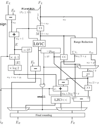
log(X) = log(Y0) +E·log 2 with Y0∈[0.75,1.5). (3) Then log(Y0) will be in the interval (−0.288,0.406). This interval is not very well centered around0, and other authors use in (2) a case boundary closer to√2, as a well-centered interval allows for a better approximation by a polynomial. We prefer that the comparison resumes to test-ing the first bit ofF, called FirstBitin the following (see Figure 1).
Now consider equation (3), and let us discuss the nor-malization of the result: We need to know which will be the exponent oflog(X). There are two mutually exclusive cases.
• EitherE6= 0, and there will be no catastrophic cancel-lation in (3). We may computeElog 2as a fixed-point value of sizewF +wE+g, whereg is a number of
guard bit to be determined. This fixed-point sum will be added to a fixed-point value oflog(Y0)onwF+1+g
bits, then a combined leading-zero-counter and barrel-shifter will determine the exponent and mantissa of the result. In this case the shift will be at most ofwEbits. • Or,E= 0. In this case the logarithm ofY0may vanish, which means that a shift to the left will be needed to normalize the result1.
– IfY0 is close enough to1, specifically ifY0 =
1 +Z0with|Z0|<2−wF/2, the left shift may be predicted thanks to the Taylor serieslog(1+Z)≈
Z − Z2/2: Its value is the number of lead-ing zeroes (if FirstBit=0) or leading ones
(ifFirstBit=1) ofY0. We actually perform
the shift before computing the Taylor series, to maximize the accuracy of this computation. Two shifts are actually needed, one onZ and one on
Z2, as seen on Figure 1.
– Or, E = 0 butY0 is not sufficiently close to1 and we have to use a range reduction, knowing that it will cancel at mostwF/2significant bits.
The simpler is to use the same LZC/barrel shifter than in the first case, which now has to shift by
wE+wF/2.
Figure 1 depicts the corresponding architecture. A detailed error analysis will be given in 4.3.
4.2
Multiplicative range reduction
This section describes the work performed by the box labelled Range Reductionon Figure 1. Consider the cen-tered mantissa Y0. If FirstBit= 0, Y0 has the form
1.0xx...xx, and its logarithm will eventually be
posi-tive. IfFirstBit= 1,Y0has the form0.11xx...xx (where the first1is the former implicit 1 of the floating-point format), and its logarithm will be negative.
Let A0 be the first 5 bits of the mantissa (including
FirstBit). A0 is used to index a table which gives an
approximationYg−1
0 of the reciprocal ofY0on 6 bits. Not-ingfY0the mantissa where the bits lower than those ofA0 are zeroed (Yf0= 1.0aaaaaorfY0= 0.11aaaaa, depending
onFirstBit), the first reciprocal table stores
1This may seem a lot of shifts to the reader. Consider that there are
barrel shifters in all the floating-point adders: In a software logarithm, there are many more hidden shifts, and one pays for them even when one doesn’t use them.
L0/1C FirstBit 0 1 0 0 Final rounding 1 small 1 Range Reduction +/− −/+ +/− = 0? −p last ×log 2 × ±1 Z2 LZC/<< EX FX E0 M 1 +wF 1 sign E E0 <0? |E| wE wE+ 1 2 +wF wF wE+wF+g1 (FX≥1.5) wF+g wF/2 +g 3wF/2 +g ER FR SR wE+ 3wF/2 +g wF+g Zlast PL i
Figure 1. Overview of the logarithm
g Y0−1= 2−5 26 f Y0 (4) The reader may check that these values ensure Y0 ×
g
Y0−1 ∈ [1,1 + 2−4]. Therefore we defineY1= 1 +Z1 =
Y0×Yg−1
0 and0 ≤ Z1 < 2−p1, withp1 = 4. The mul-tiplicationY0×Yg0−1is a rectangular one, since Yg
−1 0 is a 6-bit only number. A0 is also used to index a first loga-rithm table, that contains an accurate approximationL0of
log(Yg−1
0 )(the exact precision will be given later). This pro-vides the first step of an iteration similar to (1):
log(Y0) = log(Y0×Yg−1 0 )−log(Yg −1 0 ) = log(1 +Z1)−log(Yg0−1) = log(Y1)−L0 (5)
and the problem is reduced to evaluatinglog(Y1).
The following iterations will similarly build a sequence
Yi = 1 +Ziwith0 ≤Zi < 2−pi. Note that the sign of
log(Y0)will always be given by that ofL0, which is itself entirely defined byFirstBit. However,log(1 +Z1)will be non-negative, as will be all the following Zi (see
Fig-ures 2 and 3).
Let us now define the general iteration, starting from
i = 1. Let Ai be the subword composed of the αi
lead-Y0 : 1.0011001100110011001100110 t=0 Z1 : 00110011001100110011000010 t=2 Z2 : 010101011001100110000100001101 t=4 Z3 : 011010110100101011101110110 t=6 Z4 : 100110100000110110110010 t=8 Z4Sq : 0101110010 t=9 LogY4 : 100110100000110001000000 t=10 L0 : .0010101101111110100000001101011010101 t=1 L1 : 001010000011001001010011111100101 t=3 L2 : 010010000001010001000111100110 t=5 L3 : 010110000000001111001000001 t=7 LogY0 : .0010111010101100100111111111100100001 t=11
Figure 2. Single-precision computation of
log(Y0)forY0= 1.2
ing bits ofZi(bits of absolute weight2−pi−1to2−pi−αi).
Ai will be used to address the logarithm tableLi. As
sug-gested in Section 3, we chooseαi = 4 ∀i >0to minimize
resource usage, but another choice could lead to a different area/speed tradeoff. For instance, the architecture by Wong and Goto [24] takesαi = 10. Note that we usedα0 = 5, becauseα0= 4would lead top1= 2, which seems a worse tradeoff.
The following iterations no longer need a reciprocal ta-ble: An approximation of the reciprocal ofYi = 1 +Zi is
defined by
g
Yi−1= 1−Ai+i. (6)
The termiis a single bit that will ensureYgi−1×Yi≥1.
We define it as
i= 2−pi−αi ifαi+ 1≥piandM SB(Ai) = 0
i= 2−pi−αi−1 otherwise
(7) With definitions (6) and (7), it is possible to show that the following holds:
0 ≤ Yi+1= 1+Zi+1=Yg−1
i ×Yi < 1+2−pi−αi+1 (8)
The proof is not difficult, considering (9) below, but is too long to be exposed here. Note that (7) is inexpensive to implement in hardware: The caseαi+ 1 ≥pihappens at
most once in practice, and2−pi−αi−1is one half-ulp ofA
i.
In other words, (8) ensures pi+1 = pi +αi−1. Or,
usingαibits of table address, we are able to zero outαi−1
bits of our argument. This is slightly better than [24] where
αi −2 bits are zeroed. Approaches inspired by division
algorithms [10] are able to zeroαibits (one radix-2αidigit),
but at a higher hardware cost due to the need for signed digit arithmetic.
With αi = 4on an FPGA, the main cost is not in the
Li table (at most one LUT per table output bit), but in the
multiplication. However, a full multiplication is not needed. NotingZi=Ai+Bi(Biconsists of the lower bits ofZi),
Z0 : 0.11110011001100110011001100110011001100110011001100110 Z1 : 100111111111111111111111111111111111111111111111110010 Z2 : 110101111111111111111111111111111111111111111110010011100000 Z3 : 011101010111001111111111111111111111111111110010100001010011000100000 Z4 : 011010110100000010010001101111111111111110010100001101000111101111001 Z5 : 100110011111101101010110011100110111011000100001101011010010000110 Z6 : 100011111101100000100101001011111000000110100010101100101111110 Z7 : 101111101100000011100110000011101011101110100111010100110001 Z8 : 101101100000011100100000110100000000101001011011011000110 Z9 : 011100000011100100000100101000101000000000100100111101 Z9Sq : 0011000100110001111100001 LogY9 : 011100000011100100000100101000001111011010010101011100 L0 : -0.001011011110000110100101000101011100101011010110100101110011011111001001001100110 L1 : 100000100000101011101100010011110011101000100010001000111000000010111001111000 L2 : 110010001001110011100011100000100101011001101101111001011000011100100110100 L3 : 011010000000010101001000010110111001000110100100010010111100000000111110 L4 : 010110000000000001111001000000001101110111010111000111101110000101000 L5 : 100010000000000000100100001000000000110011001011010110100110111001 L6 : 011110000000000000000011100001000000000000100011001010000000000 L7 : 101010000000000000000000110111001000000000000001100000011110 L8 : 101010000000000000000000000110111001000000000000000001100 LogY0 : -0.000110100100001100011101010110111100110000011001001111100100101101101001100010101
Figure 3. Double-precision computation oflog(Y0)forY0= 0.95.
we have1 +Zi+1 =Yg−1
i ×(1 +Zi) = (1−Ai+i)×
(1 +Ai+Bi), hence
Zi+1=Bi−AiZi+i(1 +Zi) (9)
Here the multiplication byiis just a shift, and the only real
multiplication is the productAiZi: The full computation of
(9) amounts to the equivalent of a rectangular multiplication of(αi+ 2)×sibits. Heresiis the size ofZi, which will
vary betweenwF and3wF/2(see below).
An important remark is that (8) still holds if the product is truncated. Indeed, in the architecture, we will need to truncate it to limit the size of the computation datapath. Let us now address this question.
We will stop the iteration as soon asZiis small enough
for a second-order Taylor formula to provide sufficient accuracy (this also defines the threshold on leading ze-roes/ones at which we choose to use the path computing
Z0−Z02/2directly). Inlog(1 +Zi)≈Zi−Zi2/2 +Zi3/3,
with Zi < 2−pi, the third-order term is smaller than
2−3pi−1. We therefore stop the iteration atp
maxsuch that
pmax ≥ dw2Fe. This sets the target absolute precision of the whole datapath topmax+wF +g ≈ d3wF/2e+g.
The computation defined by (9) increases the size of Zi,
which will be truncated as soon as its LSB becomes smaller than this target precision. Figures 2 and 3 give an in-stance of this datapath in single and double precision re-spectively. Note that the architecture counts as many rect-angular multipliers as there are stages, and may therefore be fully pipelined. Reusing one single multiplier would be possible, and would save a significant amount of hardware, but a high-throughput architecture is preferable.
Finally, at each iteration,Aiis also used to index a
log-arithm tableLi(see Figures 2 and 3). All these logarithms
have to be added, which can be done in parallel to the re-duction of1 +Zi. The output of theRange Reductionbox
is the sum ofZmaxand this sum of tabulated logarithms, so it only remains to subtract the second-order term (Figure 1).
4.3
Error analysis
We computeElog 2withwE+wF+g1precision, and the sumElog 2 + logY0 cancels at most one bit, sog1 =
2 ensures faithful accuracy of the sum, assuming faithful accuracy oflogY0.
In general, the computation oflogY0is much too accu-rate: As illustrated by Figure 2, the most significant bit of the result is that of the first non-zeroLi(L0in the example), and we have computed almostwF/2bits of extra accuracy.
The errors due to the rounding of the Li and the
trunca-tion of the intermediate computatrunca-tions are absorbed by this extra accuracy. However, two specific worst-case situation require more attention.
• WhenZ0 < 2−pmax, we compute logY0 directly as
Z0−Z02/2, and this is the sole source of error. The shift that brings the leading one of |Z0| in positionpmax ensures that this computation is done onwF +gbits,
hence faithful rounding.
• The real worst case is whenY0 = 1−2−pmax+1: In this case we use the range reduction, knowing that it will cancel pmax −1 bits of L0 one one side, and accumulate rounding errors on the other side. We havemaxstages, each contributing at most3ulps of error: To compute (9), we first truncate Zi to
min-imize multiplier size, then we truncate the product, and also truncate i(1 + Zi). Therefore we need
g=dlog2(3×max)eguard bits. For double-precision, this givesg= 5.
4.4
Remarks on the
Litables
When one looks at theLi tables, one notices that some
of their bits are constantly zeroes: Indeed they holdLi ≈
log(1−(Ai−i))which can for largeribe approximated
by a Taylor series. We chose to leave the task of optimiz-ing out these zeroes to the logic synthesizer. A natural idea
would also be to store onlylog(1−(Ai−i)) + (Ai−i),
and constructLiout of this value by subtracting(Ai−i).
However, the delay and LUT usage of this reconstruction would in fact be higher than that of storing the correspond-ing bits. As a conclusion, with the FPGA target, the simpler approach is also the better. The same remark will apply to the tables of the exponential operator.
5
A hardware exponential algorithm
5.1
Initial range reduction
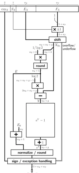
The range reduction for the exponential operator is di-rectly inspired from the method presented in [7]. The first step transforms the floating-point input X into a fixed-point number Xfix thanks to a barrel shifter. Indeed, if
EX > wE −1 + log2(log 2), then the result overflows, while ifEX <0, thenX is close to zero and its
exponen-tial will be close to1 +X, so we can loose the bits ofXof absolute weight smaller than2−wF−g,gbeing the number
of guard bits required for the operator (typically3to5bits). ThusXfixwill be awE+wF +g-bit number, obtained by
shifting the mantissa1.FX by at mostwE−1bits on the
left andwF+gbits on the right.
This fixed-point number is then reduced in order to ob-tain an integer E and a fixed-point number Y such that
X ≈ E ·log 2 +Y and0 ≤ Y < 1. This is achieved by first multiplying the most significant bits ofXfix by an approximation to1/log 2and then truncating the result to obtainE. ThenY is computed asXfix−E·log 2, requiring a rectangular multiplier.
After computingeY thanks to the iterative algorithm de-tailed in the next section, we haveeX ≈eXfix ≈eY ·2E,
and a simple renormalization and rounding step recon-structs the final result. The approximation to 1/log 2 is chosen so that this step shifts by at most one bit.
Figure 4 presents the overall architecture of the exponen-tial operator. Details for the computation ofeY−1are given
in Figure 5 and presented in the next section.
5.2
Iterative
range
reduction
for
the
fixed-point exponential
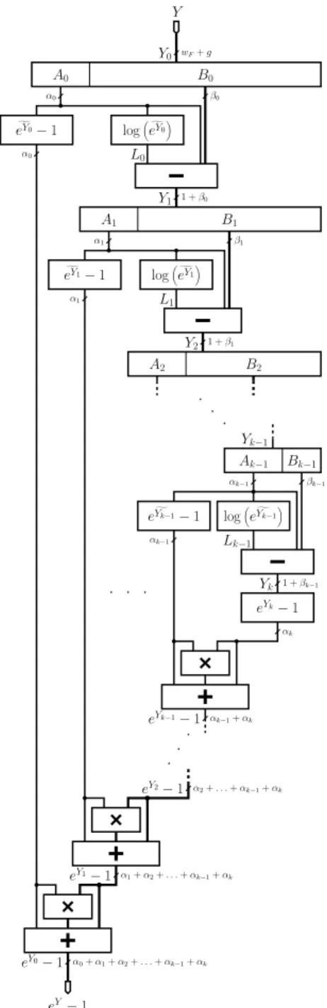
Starting with the fixed-point operand Y ∈ [0,1), we compute eY −1 using a refinement of (1). LetY0 = Y. Each iteration will start with a fixed-point numberYi and
computeYi+1closer to0, untilYkis small enough to
evalu-ateeYk−1thanks to a simple table or a Taylor
approxima-tion.
At each iteration, Yi, as for the logarithm operator, is
split into subwordsAiandBiofαiandβibits respectively.
Ai addresses two tables (again, the choice of αi = mfor
most iterations will optimize FPGA resource usage). The
wF+g eY 1 2 1 exnX SX wE FX wF EX 1 1 +wF ±1 2 +wF shift wE+wF+g Xfix round 1/log 2 wE+ 1 wE+ 4 wE+ 2 log 2 wE+wF+g−1 2wE+wF+g wF+g Y wE E0 wE+ 1 E overflow/ underflow 3 +wE+wF sign / exception handling
normalize / round
f
R≈eX
eY−1
Figure 4. Overview of the exponential
first table holds approximations ofeYi−1rounded to only αibits, which we noteefYi−1. The second one holdsLi=
logefYi
rounded toαi+βibits.
ObviouslyLi is quite close toYi. One may check that
computingYi+1as the differenceYi−Liwill result in
can-celling theαi−1most significant bits ofYi. The number
Yi+1fed into the next iteration is therefore a1+βi-bit
num-ber.
The reconstruction of the exponential uses the following recurrence with decreasingi:
f eYi−1 × eYi+1−1+ f eYi−1 + eYi+1−1 =efYi·eYi+1−1 = efYi·eYi−Li−1 =efYi·eYi·e−log “ g eYi” −1 =eYi−1.
HereeYi+1 −1comes from the previous iterations, and f
eYi−1is anαi-bit number, so the product needs a
rectan-gular multiplier.
This way, theksteps of reconstruction finally give the resulteY0−1 =eY −1. The detailed architecture of this
iterative method is presented Figure 4.
We have performed a detailed error analysis of this al-gorithm to ensure the faithful rounding of the final result. Due to space restrictions, this analysis is not presented in this article. 1 +β1 Y2 A0 B0 α0 β0 g eY0−1 logegY0 A1 B1 α0 α1 α1 g eY1−1 L1 β1 Y0 Y1 1 +β0 L0 B2 A2 logegY1 α2+. . .+αk−1+αk eY2−1 eY1−1 α1+α2+. . .+αk−1+αk eY0−1 α0+α1+α2+. . .+αk−1+αk Ak−1 Bk−1 Lk−1 αk−1 Yk−1 log g eYk−1 αk−1 βk−1 1 +βk−1 Yk g eYk−1−1 αk eYk−1 eYk−1−1 αk−1+αk wF+g . . . . . . .. . Y eY−1 Figure 5. Computation ofeY −1
6
Area and performance
The presented algorithms are implemented as C++ pro-grams that, givenwE,wF and possibly theαi, compute the
various parameters of the architecture, and output synthe-sisable VHDL. Some values of area and delay (obtained us-ing Xilinx ISE/XST 8.2 for a Virtex-II XC2V1000-4 FPGA) are given in Table 1 (where asliceis a unit containing two LUTs).
As expected, the operators presented here are smaller but slower than the previously reported ones. More importantly, their size is more or less quadratic with the precision, in-stead of exponential for the previously reported ones. This allows them to scale up to double-precision. For compar-ison, the FPGA used as a co-processor in the Cray XD1 system contains more than 23,616 slices, and the current largest available more than 40,000, so the proposed opera-tors consume about one tenth of this capacity. To provide another comparison, our operators consume less than twice the area of an FP multiplier for the same precision reported in [22].
Exponential
Format This work Previous [7]
(wE, wF) Area Delay Area Delay
(7, 16) 472 118 480 69 (8, 23) 728 123 948 85 (9, 38) 1242 175 – – (11, 52) 2045 229 – –
Logarithm
Format This work Previous [6]
(wE, wF) Area Delay Area Delay
(7, 16) 556 70 627 56 (8, 23) 881 88 1368 69 (9, 38) 1893 149 – – (11, 52) 3146 182 – –
Table 1. Area (in Virtex-II slices) and delay (in ns) of implementation on a Virtex-II 1000
These operators will be easy to pipeline to function at the typical frequency of FPGAs—100MHz for the middle-range FPGAs targeted here, 200MHz for the best current ones. This is the subject of ongoing work. The pipeline depth is expected to be quite long, up to about 30 cycles for double precision, when a double-precision multiplier is typ-ically about 10 cycles. It will also neead about 10% more slices. As mentioned in [7] and [6], one exponential or log-arithm per cycle at 100MHz is ten times the throughput of a 3GHz Pentium, and comparable to peak Itanium-II per-formance [3] using loop-optimized elementary functions. However, the proposed functions consume only a fraction of the FPGA resources.
7
Conclusion and future work
By retargeting an old family of algorithms to the spe-cific fine-grained structure of FPGAs, this work shows that elementary functions up to double precision can be imple-mented in a small fraction of current FPGAs. The resulting operators have low resource usage and high troughput, but long latency, which is not really a problem for the envi-sioned applications.
FPGAs, when used as co-processors, are often limited by their input/output bandwidth to the processor. From an ap-plication point of view, the availability of compact elemen-tary functions for the FPGA, bringing elemenelemen-tary functions on-board, will also help conserve this bandwidth.
The same principles can be used to compute sine and co-sine and their inverses, using the complex identity ejx =
cosx+jsinx. The architectural translation of this iden-tity, of course, is not trivial. Besides the main cost with trigonometric functions is actually in the argument reduc-tion involving the transcendental number π. It probably makes more sense to implement functions such assin(πx)
andcos(πx). A detailed study of this issue is also the sub-ject of current work.
References
[1] C. S. Anderson, S. Story, and N. Astafiev. Accurate math functions on the intel IA-32 architecture: A performance-driven design. In 7th Conference on Real Numbers and Computers, pages 93–105, 2006.
[2] ANSI/IEEE. Standard 754-1985 for Binary Floating-Point Arithmetic (also IEC 60559). 1985.
[3] M. Cornea, J. Harrison, and P. Tang. Scientific Computing on Itanium-based Systems. Intel Press, 2002.
[4] M. Cosnard, A. Guyot, B. Hochet, J. M. Muller, H. Ouaouicha, P. Paul, and E. Zysmann. The FELIN arith-metic coprocessor chip. In Eighth IEEE Symposium on Computer Arithmetic, pages 107–112, 1987.
[5] M. deLorimier and A. DeHon. Floating-point sparse matrix-vector multiply for FPGAs. InACM/SIGDA Field-Programmable Gate Arrays, pages 75–85. ACM Press, 2005.
[6] J. Detrey and F. de Dinechin. A parameterizable floating-point logarithm operator for FPGAs. In39th Asilomar Con-ference on Signals, Systems & Computers. IEEE Signal Pro-cessing Society, Nov. 2005.
[7] J. Detrey and F. de Dinechin. A parameterized floating-point exponential function for FPGAs. In IEEE International Conference on Field-Programmable Technology (FPT’05). IEEE Computer Society Press, Dec. 2005.
[8] J. Detrey and F. de Dinechin. Table-based polynomials for fast hardware function evaluation. In16th Intl Conference on Application-specific Systems, Architectures and Proces-sors. IEEE Computer Society Press, July 2005.
[9] Y. Dou, S. Vassiliadis, G. K. Kuzmanov, and G. N. Gay-dadjiev. 64-bit floating-point FPGA matrix multiplication. In ACM/SIGDA Field-Programmable Gate Arrays. ACM Press, 2005.
[10] M. Ercegovac. Radix-16 evaluation of certain elementary functions. IEEE Transactions on Computers, C-22(6):561– 566, June 1973.
[11] M. D. Ercegovac and T. Lang. Digital Arithmetic. Morgan Kaufmann, 2003.
[12] P. Farmwald. High-bandwidth evaluation of elementary functions. InFifth IEEE Symposium on Computer Arith-metic, pages 139–142, 1981.
[13] H. Hassler and N. Takagi. Function evaluation by table look-up and addition. In12th IEEE Symposium on Computer Arithmetic, pages 10–16, Bath, UK, 1995. IEEE.
[14] ISO/IEC. International Standard ISO/IEC 9899:1999(E). Programming languages – C. 1999.
[15] D. Lee, A. Gaffar, O. Mencer, and W. Luk. Optimizing hard-ware function evaluation.IEEE Transactions on Computers, 54(12):1520–1531, Dec. 2005.
[16] G. Lienhart, A. Kugel, and R. M¨anner. Using floating-point arithmetic on FPGAs to accelerate scientific N-body simu-lations. InFPGAs for Custom Computing Machines. IEEE, 2002.
[17] J.-M. Muller.Elementary Functions, Algorithms and Imple-mentation. Birkh¨auser, 2 edition, 2006.
[18] G. Paul and M. W. Wilson. Should the elementary functions be incorporated into computer instruction sets?ACM Trans-actions on Mathematical Software, 2(2):132–142, June 1976.
[19] J. Stine and M. Schulte. The symmetric table addition method for accurate function approximation. Journal of VLSI Signal Processing, 21(2):167–177, 1999.
[20] P. T. P. Tang. Table-driven implementation of the exponen-tial function in IEEE floating-point arithmetic.ACM Trans-actions on Mathematical Software, 15(2):144–157, June 1989.
[21] P. T. P. Tang. Table-driven implementation of the logarithm function in IEEE floating-point arithmetic. ACM Trans-actions on Mathematical Software, 16(4):378 – 400, Dec. 1990.
[22] K. Underwood. FPGAs vs. CPUs: Trends in peak floating-point performance. In ACM/SIGDA Field-Programmable Gate Arrays. ACM Press, 2004.
[23] W. F. Wong and E. Goto. Fast evaluation of the elementary functions in double precision. InTwenty-Seventh Annual Hawaii International Conference on System Sciences, pages 349–358, 1994.
[24] W. F. Wong and E. Goto. Fast hardware-based algorithms for elementary function computations using rectangular multi-pliers. IEEE Transactions on Computers, 43(3):278–294, Mar. 1994.
[25] W. F. Wong and E. Goto. Fast evaluation of the elementary functions in single precision. IEEE Transactions on Com-puters, 44(3):453–457, Mar. 1995.
[26] C. Wrathall and T. C. Chen. Convergence guarantee and im-provements for a hardware exponential and logarithm eval-uation scheme. InFourth IEEE Symposium on Computer Arithmetic, pages 175–182, 1978.