1 Page 1-10 © MAT Journals 2017. All Rights Reserved
Comparison between Different Methods used in MFCC for
Speaker Recognition System
S G Bagul
Late G. N. Sapkal, C. O. E, Nashik, India E-mail: [email protected]
Abstract
The idea of the Speaker Recognition Project is to implement a recognizer which might determine an individual by process his/her voice. The essential goal of the project is to acknowledge and classify the speeches of various persons. This classification is especially supported extracting many key options like Mel Frequency Cepstral Coefficients (MFCC) from the speech signals of these persons by mistreatment methodology of feature extraction method. The on top of options could encompass pitch, amplitude, frequency etc. employing an applied math model like gaussian mixture model (GMM) and options extracted from those speech signals we have a tendency to build a novel identity for every one that listed for speaker recognition. Estimation and Maximization formula is employed, a chic and powerful methodology for locating the most chance answer for a model with latent variables, to check the later speakers against the information of all speakers who listed within the information. Use of divisional Fourier rework for feature extraction is additionally recommended to enhance the speaker recognition potency.
Keywords: Speaker recognition, feature extraction, statistical model, gaussian mixture model, mel frequency cepstral coefficients, fractional fourier transform
INTRODUCTION
This project encompasses the implementation of Text freelance speaker recognition. Speaker recognition systems are often characterized as text-dependent or text-independent. The system we have developed is the latter, text-independent, that means the system will determine the speaker in spite of what is being aforesaid. The program can contain 2 functionalities: A coaching mode, a recognition mode. The coaching mode can permit the user to record voice and create a feature model of that voice. The popularity mode can use the knowledge that the user has provided within the coaching mode and conceive to isolate and determine the speaker. Most people square measure attentive to the very fact that voices of various people do not sound alike. This vital property of speech-of being speaker dependent-is what allows us to recognize an addict over a telephone. Speech is usable for
identification as a result of it is a product of the speaker’s individual anatomy and linguistic background [1]. In additional specific, the speech signal created by a given individual is full of each the organic characteristics of the speaker (in terms of vocal tract geometry) and learned variations attributable to ethnic or social factors. To consider the above concept as a basic, we have establisheda “Speaker Recognition System. Speaker recognition can be classified into identification and verification. Speaker identificationis the process of determining which registered speaker provides a given utterance. Speaker verification, on the other hand, is the process of accepting or rejecting the identity claim of a speaker. The system that we will describe is classified as text-independent speaker identificationsystem since its task is to identify the person who speaks regardless of what is saying [1].
2 Page 1-10 © MAT Journals 2017. All Rights Reserved In this paper, we are going to discuss
solely the text freelance, however, speaker dependent Speaker Recognition system. All technologies of speaker recognition, identification and verification, text-independent and text dependent, every has its own benefits and downsides and will need completely different treatments and techniques. The choice of that technology to use is application-specific. At the very best level, all speaker recognition systems contain 2 main modules: feature extraction and have matching. Feature extraction is that the method that extracts a little quantity of information from the voice signal that may later be wont to represent every speaker. Feature matching involves the particular procedure to spot the unknown speaker by comparison extracted options from his/her voice input with those from a collection of noted speakers [2]. A wide vary of prospects exist for parametrically representing the speech signal for the speaker recognition task, like Linear Prediction coding (LPC), Mel-Frequency Cepstrum Coefficients (MFCC). LPC analyzes the speech signal by estimating the formants, removing their effects from the speech signal, and estimating the intensity and frequency of the remaining buzz. The method of removing the formants is named inverse filtering, and also the remaining signal is named the residue. Another widespread speech feature illustration is understood as RASTA-PLP, an acronym for Relative Spectral rework-sensory activity Linear Prediction. PLP was originally planned by Hynek Hermansky as the way of warp spectra to attenuate the variations between speakers whereas conserving the necessary speech data. RASTA is a separate technique that applies a band-pass filter to the energy in each frequency sub band in order to smooth over short-term noise variations and to remove any constant offset resulting from static spectral coloration in the speech channel, e.g., from
a telephone line [3]. Many approaches have been proposed for TI speaker recognition. First is the VQ based method which uses VQcodebooks as an efficient means of characterizing speaker specific feature [1]. An input utterance is first vector-quantized.
Using the codebook of each reference speaker, and the VQdistortion is used for making recognition decision. To bettermodeling the acoustic feature and incorporate the temporalstructure modeling, the Hidden Markov Models (HMM) havebeen used as probabilistic speaker model for both TI and TDtasks. Poritz proposed a five state ergodic HMM, which classify acoustic events into broad phonetic categoriescorresponding to HMM states, to characterize each speaker in task [2]. However, Matsui found that TI performance wasunaffected by discarding transition probabilities in HMM models [3]. Rose and Reynolds introduced a methods based on Gaussian Mixture Model (GMM) (corresponds to a single state Continuousergodic HMM) to model speaker identity [3, 4]. The GMM, on the other hand, provide probabilistic model ofthe underlying acoustic properties of a person but do not impose any Markovian constraints between the acoustic classesby discarding the transition probabilities in the HMM models.The use of GMM for speaker identity modeling is motivated bythe interpretation that the Gaussian components represent somegeneral speaker-dependent spectral shapes and the capability of Gaussian mixture to model arbitrary densities. The GMM hasbeen firstly used for TI speaker identification and is extended to speaker verification on several publicly available speech corpora [5]. The GMM was also shown to outperformthe conventional Vector
Quantization (VQ) method
anddiscriminative method (Radial Basis Function) in TI speaker ID Task [5].
3 Page 1-10 © MAT Journals 2017. All Rights Reserved MFCC’s are supported the famous
variation of the human ear’s crucial bandwidths with frequency; filters spaced linearly at low frequencies and logarithmically at high frequencies are accustomed capture the phonetically vital characteristics of speech. This can be expressed within the mel-frequency scale that is linear frequency spacing below a thousand Hertz and power spacing above 1000 Hertz. MFCC is probably the most effective famous and most well-liked [2]. Here is simply summary of our approach to the current project, initial we tend to extracted options from the speech signal and so we tend to provide them to the applied math model, here we tend to use GMM as applied math model to make a novel voice print for every identity [6–9].
Fig. 1: Block Diagram of Speaker Recognition System.
After creation of all voice prints for all identities we check the data base of these voice prints against another voice print which was created by GMM using testing data [3]. In this project, the GMM approach will be used, due to ease of implementation and high accuracy.
Mel Frequency Cepstral Coefficients (MFCC)
MFCC’s are coefficients that represent audio, based on perception. It is derived from the Fourier Transform or the Discrete Cosine Transform of the audio clip. The basic difference between the FFT/DCT and the MFCC is that in the MFCC, the frequency bands are positioned logarithmically (on the mel scale) which
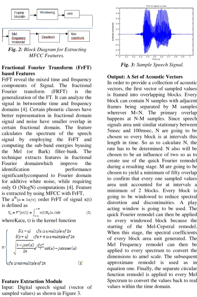
approximates the human auditory system's response more closely than the linearly spaced frequency bands of FFT or DCT. This allows for better processing of data, for example, in audio compression. The main purpose of the MFCC processor is to mimic the behaviour of the human ears [2]. The MFCC process is subdivided into five phases or blocks. In the frame blocking section, the speech waveform is more or less divided into frames of approximately 30 milliseconds. The windowing block minimizes the discontinuities of the signal by tapering the beginning and end of each frame to zero. The FFT block converts each frame from the time domain to the frequency domain. In the Mel frequency wrapping block, the signal is plotted against the Mel-spectrum to mimic human hearing. Studies have shown that human hearing does not follow the linear scale but rather the Mel-spectrum scale which isa linear spacing below 1000 Hz and logarithmic scaling above 1000 Hz. In the final step, the Mel-spectrum plot is converted back to the time domain by using the following equation: The resultant matrices are remarked because the Mel-Frequency Cepstrum Coefficients. This spectrum provides a reasonably easy, however, distinctive illustration of the spectral properties of the voice signal that is that the key for representing and recognizing the voice characteristics of the speaker [10]. A speaker voice patterns could exhibit a considerable degree of variance: identical sentences, spoken by a similar speaker, however, at totally different times, lead to an analogous, nonetheless totally different sequence of MFCC matrices. The aim of speaker modeling is to make a model which will address speaker variation in feature house and to form a reasonably distinctive illustration of the speaker's characteristics [11].
4 Page 1-10 © MAT Journals 2017. All Rights Reserved
Fig. 2: Block Diagram for Extracting MFCC Features.
Fractional Fourier Transform (FrFT) based Features
FrFT reveal the mixed time and frequency components of Signal. The fractional Fourier transform (FRFT) is the generalization of the FT. It can analyze the signal in betweenthe time and frequency domains [4]. Certain phonetic classes have better representation in fractional domain signal and noise have smaller overlap in certain fractional domain. The feature calculates the spectrum of the speech signal by employing the FrFT and computing the sub-band energies byusing the Mel (or Bark) filter-bank. The technique extracts features in fractional Fourier domainwhich improve the
identification performance
significantlycompared to Fourier domain for additive white noise, while requiring only O (NlogN) computations [4]. Feature is extracted by using MFCC with FrFT, The ath order FrFT of signal x(t) is defined as
whereKa(u, t) is the kernel function
Feature Extraction Module
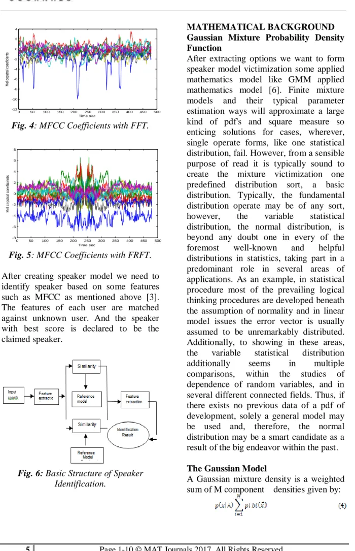
Input: Digital speech signal (vector of sampled values) as shown in Figure 3.
0 0.1 0.2 0.3 0.4 0.5 0.6 0.7 0.8 0.9 1 -0.4 -0.3 -0.2 -0.1 0 0.1 0.2 0.3 0.4 0.5
Plot of signal s1.wav
Time [s] A m pl itu de ( no rm al iz ed )
Fig. 3: Sample Speech Signal.
Output: A Set of Acoustic Vectors
In order to provide a collection of acoustic vectors, the first vector of sampled values is framed into overlapping blocks. Every block can contain N samples with adjacent frames being separated by M samples wherever M<N. The primary overlap happens at N-M samples. Since speech signals area unit similar stationary between 5msec and 100msec, N are going to be chosen so every block is at intervals this length in time. So as to calculate N, the rate has to be determined. N also will be chosen to be an influence of two so as to create use of the quick Fourier remodel during a resulting stage. M are going to be chosen to yield a minimum of fifty overlap to confirm that every one sampled values area unit accounted for at intervals a minimum of 2 blocks. Every block is going to be windowed to reduce spectral distortion and discontinuities. A play acting window is going to be used. The quick Fourier remodel can then be applied to every windowed block because the starting of the Mel-Cepstral remodel. When this stage, the spectral coefficients of every block area unit generated. The Mel Frequency remodel can then be applied to every spectrum to convert the dimensions to amel scale. The subsequent approximate remodel is used as in equation one. Finally, the separate circular function remodel is applied to every Mel Spectrum to convert the values back to real values within the time domain.
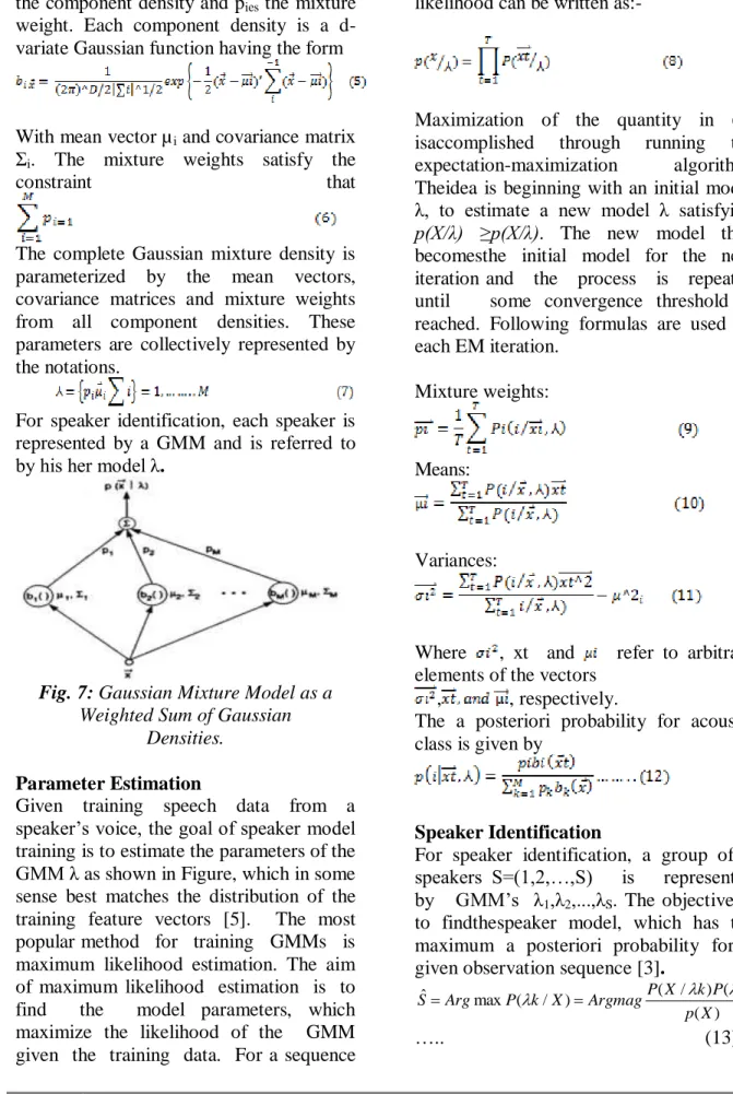
5 Page 1-10 © MAT Journals 2017. All Rights Reserved 0 50 100 150 200 250 300 350 400 450 500 -12 -10 -8 -6 -4 -2 0 2 4 Time sec M el c ep st ra l c oe ef ic ie nt s
Fig. 4: MFCC Coefficients with FFT.
0 50 100 150 200 250 300 350 400 450 500 -8 -6 -4 -2 0 2 4 6 8 Time sec M el c ep st ra l c oe ef ic ie nt s
Fig. 5: MFCC Coefficients with FRFT. After creating speaker model we need to identify speaker based on some features such as MFCC as mentioned above [3]. The features of each user are matched against unknown user. And the speaker with best score is declared to be the claimed speaker.
Fig. 6: Basic Structure of Speaker Identification.
MATHEMATICAL BACKGROUND Gaussian Mixture Probability Density Function
After extracting options we want to form speaker model victimization some applied mathematics model like GMM applied mathematics model [6]. Finite mixture models and their typical parameter estimation ways will approximate a large kind of pdf's and square measure so enticing solutions for cases, wherever, single operate forms, like one statistical distribution, fail. However, from a sensible purpose of read it is typically sound to create the mixture victimization one predefined distribution sort, a basic distribution. Typically, the fundamental distribution operate may be of any sort, however, the variable statistical distribution, the normal distribution, is beyond any doubt one in every of the foremost well-known and helpful distributions in statistics, taking part in a predominant role in several areas of applications. As an example, in statistical procedure most of the prevailing logical thinking procedures are developed beneath the assumption of normality and in linear model issues the error vector is usually assumed to be unremarkably distributed. Additionally, to showing in these areas, the variable statistical distribution additionally seems in multiple comparisons, within the studies of dependence of random variables, and in several different connected fields. Thus, if there exists no previous data of a pdf of development, solely a general model may be used and, therefore, the normal distribution may be a smart candidate as a result of the big endeavor within the past.
The Gaussian Model
A Gaussian mixture density is a weighted sum of M component densities given by:
6 Page 1-10 © MAT Journals 2017. All Rights Reserved Where x is a d-dimensional vector, bi(x) is
the component density and pies the mixture
weight. Each component density is a d-variate Gaussian function having the form
With mean vector µi and covariance matrix
Σi. The mixture weights satisfy the
constraint that
The complete Gaussian mixture density is parameterized by the mean vectors, covariance matrices and mixture weights from all component densities. These parameters are collectively represented by the notations.
For speaker identification, each speaker is represented by a GMM and is referred to by his her model λ.
Fig. 7: Gaussian Mixture Model as a Weighted Sum of Gaussian
Densities.
Parameter Estimation
Given training speech data from a speaker’s voice, the goal of speaker model training is to estimate the parameters of the GMM λ as shown in Figure, which in some sense best matches the distribution of the training feature vectors [5]. The most popular method for training GMMs is maximum likelihood estimation. The aim of maximum likelihood estimation is to find the model parameters, which maximize the likelihood of the GMM given the training data. For a sequence
of T training vectors X=(x1, xT) the GMM
likelihood can be written as:-
Maximization of the quantity in (8) isaccomplished through running the expectation-maximization algorithm. Theidea is beginning with an initial model λ, to estimate a new model λ satisfying p(X/λ) ≥p(X/λ). The new model then becomesthe initial model for the next iteration and the process is repeated until some convergence threshold is reached. Following formulas are used on each EM iteration.
Mixture weights:
Means:
Variances:
Where , xt and refer to arbitrary elements of the vectors
, , respectively.
The a posteriori probability for acoustic class is given by
Speaker Identification
For speaker identification, a group of S speakers S=(1,2,…,S) is represented by GMM’s λ1,λ2,...,λS. The objective is
to findthespeaker model, which has the maximum a posteriori probability for a given observation sequence [3].
) ( ) ( ) / ( ) / ( max ˆ X p K P k X P Argmag X k P Arg S ….. (13)
7 Page 1-10 © MAT Journals 2017. All Rights Reserved Wherethe second equation is due to
Bayes’srule. Assuming equally likely speakers (P(λk)= 1/S) and noting that p(X)
is the same for all speaker models, the classification becomes: ) / ( max ˆ Arg P X k S (14)
Finally with logarithms,the speaker identification system gives:
T t k xt P Arg S 1 ) / ( log max ˆ (15) In which p(xt/λk) is given in equation 4.Performance Evaluation
Evaluation of a speaker identification experiment is conducted as follows. The test speech is first processed by the front-end analysis to produce a sequence of spectral vectors (x1,...,xT) . Different test utterancesof
length 2, 5 and 10 seconds were used each having a number of T feature vectors. Performance evaluation is then computedduring the Identification Error Rate (IER) given by equation 4.
EXPERIMENTAL RESULTS AND
ANALYSIS
The database for system evaluation consists of phonetically balanced sentences utterances by 30 male and 10 female client speakers age 16-24yrs with each provides the same 40 sentences utterances with different text. This database was recorded on one session in the same recording room with same microphone for all speakers for all sessions. The average sentences duration is approximately 3.5 s. Train (22 to 35sec) and Test (3 to 7 sec) A subset of sentences is used for training the speaker specific model. The other subset is used for testing. The training sentences with different text are same for all speakers. The testing sentences were different from those for training but same for all speakers. For identification, an unknown speech signal
which has been transformed into MFC feature pattern is classified into speaker whose GMM model gives highest likelihood. A series of experiments were established to evaluate the systems. The following experiment investigates the effect of different number of Gaussian mixture components on identification rate for different amount of training data. MFCC feature dimension is fixed to 12. The speaker models with model order varied from 1 to 32 were trained using 5, 10, and 15 training sentences. 25 sentences of different text from the training set were used for testing. Generally, for all model order, increasing the amount of training data increases the identification rate. For all amount of training data, there is a sharp increase in performance from 1 to 4 components, and start leveling off at 8 components. Compared to the relatively constant performance, for the small amount of training data (5 sentences) drops at 32 mixture components. This is because there are too many parameters to be estimated reliably with relatively insufficient training data.
8 Page 1-10 © MAT Journals 2017. All Rights Reserved
Table 1: Identification Performance without Noise.
Number Of Number Of Number % Speaker Speakers Mixture Of Identification
Components Iterations 2 87.5% 8 20 97.5% 51 100% 2 92.5% 40 16 20 97.5% 51 100% 2 97.5% 32 20 100% 51 100%
Table 2: Identification Performance with Noise.
Noise Number Of Number Of % Speaker added in Mixture Iterations Identification
Test Data Components
40 Speakers Set 2 24% 8 20 4% 15dB 51 - 2 26% 16 20 26% 51 26% 2 26% 32 20 20% 51 54%
9 Page 1-10 © MAT Journals 2017. All Rights Reserved
Table 3: Identification Performance with Temporal Derivatives. Noise Number Of Number Of % Speaker added in Mixture Iterations Identification
Test Data Components 40 Speakers Set 2 28% 8 20 30% 15dB 51 22% 2 45% 16 20 32% 51 40% 2 32% 32 20 35% 51 60% CONCLUSION
Experimental results on Created information reveal that FrFT based mostly algorithms perform higher in noisy condition whereas Mel scale based strategies perform well on clean information. The Gaussian mixture speaker model maintains high identification performance with increasing population size. These results indicate that Gaussian mixture models offer a sturdy speaker illustration for the troublesome task of speaker recognition mistreatment corrupted, free speech. The models area unit computationally cheap and simply enforced on a true time platform. What is more their probabilistic frame-work permits direct integration with speech recognition systems and incorporation of new developed speech strength techniques. Equally higher results are obtained by implementing third Fourier rework with GMM.
REFERENCES
1. J.P.Cambell,Jr., “Speaker Recognition : A Tutorial”,Proceedingsof The IEEE, vol. 85, no. 9, pp. 1437-1462, Sept. 1997.
2. RashidulHasan, MustafaJamil, Md. GolamRabbani ,“SpeakerIdentification Using Mel Frequency Cepstral
Coefficient” 3rd
InternationalConference onElectrical
& Computer
EngineeringICEC2004,28-30, Dhaka BangladeshISBN 984-32-1804
3. D.A Reynolds, R.C. Rose, “Robust text-independent speakeridentification using Gaussian mixture speaker models”, IEEE TransSpeech Audio Process., vol. 3,No.1,pp.72-83 January 1995
4. Upendra Kumar Agrawal, Mahesh Chandra, “Fractional Fourier Transform Combinationwith MFCCBased Speaker Identification in clean Environment” Badgaiyan International Journal of Advanced Science, Engineering and Technology. ISSN 2319-5924Vol 1, Issue 1, 2012
10 Page 1-10 © MAT Journals 2017. All Rights Reserved 5. Model Chee-Ming Ting,
Sh-HussainSalleh, Tian-SweeTan,“Text Independent Speaker Identification UsingGaussian Mixture”Center for Biomedical Engineering, Faculty of ElectricalEngineeringUniversity
Technology Malaysia
“InternationalConference on Intelligent and Advanced Systems 2007”.
6. Rabiner L, Juang B. H, Fundamentals of speech recognition,second Edition. 7. Speech Signal Processing,
Dr.S.D.Apte,Wiley Publication. First Edition.
8. Douglas A. Reynolds,” Automatic Speaker Recognition Using Gaussian Mixture Speaker Models” Volume B,
Number 2, 1995The Lincoln Laboratory Journal.
9. Bishnu S. Atal,” Automatic Recognition of Speakers & From Their Voices”, Proceedings of the IEEE, April 1976.
10.T. Kinnunen, H. Li, “An overview of text-independent speakerrecognition: From features to supervectors,” SpeechCommunication, vol. 52, no. 1, pp. 12-40, 2010.
11.Cagetaycandar, M.AlienKutay, member IEEE “The Discrete fractional fourier Transform” IEEE Transactions on Signal Processing, VOL. 48, NO. 5,