A Framework to Decompose GSPN Models

A Framework to Decompose GSPN Models

Pontif´ıcia Universidade Cat´olica do Rio Grande do Sul, Av. Ipiranga, 6681 – 90619-900 – Porto Alegre, Brazil {lbrenner, paulof, asales, twebber}@inf.pucrs.br

Abstract. This paper presents a framework to decompose a single GSPN model into a set of small interacting models. This decomposition technique can be applied to any GSPN model with a finite set of tangi-ble markings and a generalized tensor algebra (Kronecker) representation can be produced automatically. The numerical impact of all the possi-ble decompositions obtained by our technique is discussed. To do so we draw the comparison of the results for some practical examples. Finally, we present all the computational gains achieved by our technique, as well as the future extensions of this concept for other structured formalisms.

1

Introduction

It is common knowledge in the research community the advantages in using theGSPN (Generalized Stochastic Petri Nets) formalism [2] to model complex systems,i.e., systems with both parallel and synchronous behavior. For a quite long time, the main limitation to use theGSPN formalism was the absence of an efficient numerical support to handle useful, and consequently large, models. Ciardo and Trivedi’s work [14] brought a first approach that could be employed to decompose a single model into components. However, their approach does not mention any specific storage or numerically suitable solution technique. The need of a theoretical tool to represent such structured models naturally leads toTensor Algebra representations [4, 8, 3, 15]. The termTensor Algebra is being employed in this paper, but many authors still prefer the classic denomination Kronecker Algebra chosen in honor of Leopold Kronecker.

The first complete approaches in this direction were the works of Donatelli in theSGSPN (Superposed GSPN) formalism [16, 17]. By complete, we under-stand that it was proposed a complete framework to: construct aSGSPNmodel by assembling synchronized components; generate a Markovian descriptor,i.e., a tensor algebra formula, as the infinitesimal generator of the equivalent Markov chain; and consequently an efficient way to solve it (functional elements). How-ever, the SGSPN formalism could only be used to model a rather small class ofGSPN models which comply to the restrictive rules of generation defined by

_{This work was partially funded by CNPq/Brazil.}

_{Corresponding author. The order of authors is merely alphabetical.}

G. Ciardo and P. Darondeau (Eds.): ICATPN 2005, LNCS 3536, pp. 128–147, 2005. c

Donatelli,i.e., aSGSPNmodel is composed of a set of standardGSPN models which interact only through a set of synchronized transitions.

TheSGSPNapplication scope restriction, and the consequent disadvantages in terms of numerical performance, suggests the use of other formalisms that could be closer to the tensor representation, such asSAN(Stochastic Automata Networks) [26]. At this time, the solution through the shuffle algorithm used in SAN [18, 7] presents an efficient solution with reasonable memory needs. Evidently, the use of other structured storage and solution techniques instead of the tensor algebra also presents good alternatives to the limited scope of the

SGSPN formalism. This is the case of the quite impressive techniques based on

MDD(Multi-valued Decision Diagrams) [22] andMxD (Matrix Diagrams) [21] proposed by Ciardo and Miner. Furthermore, the MDD and MxD techniques are very efficient to solve very sparse models, i.e., models with a huge product state space and a comparatively small number of reachable states. In fact, we believe that the techniques based on tensor algebra are still worthy, at least considering the new improvements to handle tensor structures [5, 10].

This paper presents a study about the decomposition of a very general class of

GSPNmodels, exploiting the description power of theGSPNformalism. It also proposes a memory efficient tensor algebra format to describe the components and their interactions. As the first step, we formally define the class of GSPN models in which our technique can be applied. The proposed decomposition technique and the consequent tensor format representation are generalizations of theSGSPNformalism [17], but we extend the application scope following the ideas firstly advanced in [14] and employed later in [20]. The new contribution of our work is justified by the numerical impact of the decomposition choices on the storage demands.

We are specifically interested to handle models with a really large reachable state space. Buchholz, Ciardo, Donatelli, Kemper, and Miner [9, 23, 11] already present very efficient methods to deal with absolutely huge models (e.g., 9.18× 10626 states in 1000 dining philosophers example [22]), but with considerably fewer reachable states. Our decomposition technique intends to split a GSPN model into subnets providing a structured representation. Regardless the number of subnets, we will always have the same reachable state space. With many (small) subnets, we have a very structured (and therefore memory efficient) representation, but also a product state space much larger than the reachable state space. With few (large) subnets, we have a less structured representation, but a product state space equal or a little bit larger than the reachable state space. In fact, we intend to compare possible decompositions in order to show the trade off between many small and few large subnets.

In addition, we point out the underestimated benefits of the use of guards in theGSPN formalism, which can be clearly demonstrated by the tensor format proposed in our work. We do not pay much attention in this paper to the com-putational cost to solve the tensor representations. The recent evolutions in pure tensor solutions [5, 10], the promising ideas of parallel implementations, and the

cost in a near future. We focus our interest in the memory savings due to our decomposition techniques and the corresponding tensor format.

The next section briefly presents the theoretical tool used to the tensor rep-resentation: Classical (CTA) and Generalized Tensor Algebra (GTA). Section 3 describes theGSPN formalism, the application scope of our technique and the scope of the technique proposed forSGSPN. Section 4 presents our decomposi-tion technique and the corresponding tensor format. Secdecomposi-tion 5 draws some con-siderations about the possible choices of decomposition. Section 6 presents some modeling examples in order to discuss numerical issues about the decomposition technique. Finally, the conclusion summarizes our contribution and suggests the still vast future work to be done.

2

Tensor Algebra

In this section, the concepts of Classical Tensor Algebra [3, 15] and Generalized Tensor Algebra [25, 18] are briefly presented.

2.1 CTA - Classical Tensor Algebra

The tensor product of two matrices:Aof dimensions (ρ1×γ1) andB of dimen-sions (ρ2×γ2) is a tensor with dimensions (ρ1ρ2×γ1γ2) which may be considered as consisting of ρ1γ1blocks each having dimensions (ρ2γ2),i.e., the dimensions of B. To specify a particular element, it suffices to specify the block in which the element occurs and the position within that block of the element under con-sideration. Thus, as mentioned previously, element c36 (a11b02) is in the (1, 1) block and at position (0, 2) of that block. The tensorC =A⊗B is defined by assigning to the element of C that is in the (k, l) position of block (i, j), the valueaijbkl,i.e.,c[ik][jl]=aijbkl. Thetensor sumof twosquare matricesAand

B is defined in terms of tensor products as:

A⊕B=A⊗InB+InA⊗B

wherenAis the order ofA;nBis the order ofB;Iniis the identity matrix of order

ni; and “+” represents the usual operation of matrix addition. Since both sides of this operation (matrix addition) must have identical dimensions, it follows that tensor addition is defined for square matrices only. The value assigned to the elementc[ik][jl] of the tensorC=A⊕B isc[ik][jl]=aijδkl+bklδij, whereδij is the element ofith_{row andj}th_{column of an identity matrix defined asδ}

ij = 1 fori=j andδij= 0 for i=j.

2.2 GTA - Generalized Tensor Algebra

Generalized Tensor Algebra is an extension of Classical Tensor Algebra. The main distinction ofGTA with respect toCTA is the addition of the concept of functional elements. However, a matrix can be composed of constant elements

(belonging toR) or functional elements. A functional element is a function eval-uated in R according to a set of parameters composed of the rows of one or more matrices. Generalized tensor product is denoted by⊗

g. The value assigned to the elementc[ik][jl] of the tensorC=A(B)⊗

g B(A) isc[ik][jl]=aij(bk)bkl(ai). Generalized tensor sum is also analogous to the ordinary tensor sum, and is denoted by ⊕

g. The elements of the tensor C = A(B)⊕g B(A) are c[ik][jl] =

aij(bk)δkl+bkl(ai)δij.

3

Generalized Stochastic Petri Nets

TheGSPNformalism [2] is a performance analysis tool on the graphical system representation typical of Petri Nets [27, 24]. The GSPN formalism is derived from theSPN formalism and contains two types of transitions: timed and im-mediate. An exponentially distributed random firing time is associated with each timed transition, whereas immediate transitions, by definition, fire in zero time. Immediate transitions always have precedence to fire over timed transitions. The

GSPNmodels with immediate transitions can always be represented by a model with timed transitions.

In the graphical representation of aGSPNmodel, places are drawn as circles, timed transitions as rectangles and immediate transitions as bars. Places may containstokens, which are drawn as black dots. A place is an input to a transition if an arc exists from the place to the transition. A place is an output from a transition if an arc exists from the transition to the place. A transition is enabled when all of its input places contain at least one token. Enabled transitions can fire, thus removing one token from each input place and placing one token in each output place. Additionally, a condition can be associated to enable the firing of the transitions. Such conditions are called guards and, with the availability of tokens in the input places, they are the only restrictions to enable the firing of a given transition. A formal description is presented as follows.

Let

C set of conditions associated to transitions of T.

Definition 1. AGSPN is defined by tuple (P,T,π,I,O,W,G,M0), where: 1.1. P non-empty set of places;

1.2. T non-empty set of transitions;

1.3. π:T → {0,1} priority function of the transitions;

1.4. I andO:T → P input and output functions of the transitions;

1.5. W:T →R+ _{function that assigns a rate to each transition;}

1.6. G:T → C function, called guard, that associates a necessary, but not

suffi-cient, conditionc∈ C to the firing of each transitiont∈ T; 1.7. M0:P →Ninitial marking in each place.

Definition 2. c∈ Cis a condition that may be associated to a transitiont∈ T, which depends on tokens of one or morep∈ P. This condition is a function with domain on tokens of all places pand counter-domain onR.

A conditionc defines the firing rate of a transition according to the number of tokens in a specific set of places. Although the counter-domain of c is R, only a discrete set of values can be obtained, since the possible combination of markings of places (i.e., the domain ofc) is a discrete set.

Definition 3. Set of timed transitions TT of a GSPN is defined as TT ={t∈ T |π(t) = 0}.

Definition 4. Set of immediate transitions TI of a GSPN is defined asTI = {t∈ T |π(t) = 1}.

Definition 5. Set of transitionsT of a GSPN is defined as T =TT∪ TI and TT ∩ TI =∅.

Numerical Solution Restriction. Although the framework proposed in this paper could be applied to a larger class of GSPN models, we assume a single restriction in order to facilitate the stationary or transient numerical solution: the set of tangible markings of the models must be finite.

4

Framework

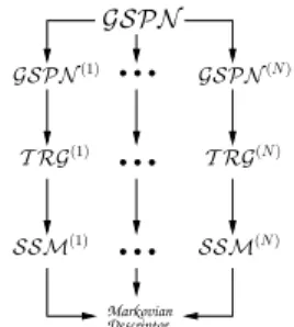
We present in this section a framework to decompose GSPN models. Our de-composition technique is shown in Fig. 1.

The basic idea is to decompose a GSPNmodel intoN componentsGSPN(i) (i∈[1..N]), where each component GSPN(i) is viewed as a subsystem of the

GSPN model. A component GSPN(i) may not be a GSPN model. It is then necessary to know the possible tangible markings. This is done by the con-struction of T RG(i) considering the possible firing of all transitions limited by: availability of tokens; guards; and maximum number of tokens in each place.

A componentGSPN(i) has an independent behavior (local transitions) and occasional interdependencies (synchronized transitions and/or transitions with guards). It is important to notice that there is a strong equivalence between the decomposition of all T RG(i) and the T RG of the whole GSPN (which is the underlying Markov Chain). Nevertheless the computational cost to obtain the T RG from the composition of all T RG(i) is usually too high. In fact, the memory needs can be prohibitive as will be seem in the Section 6.

In the next section, we define a component GSPN(i) and its properties. In Section 4.2, we formally present the tensor format (Markovian Descriptor) used to obtain the infinitesimal generatorQof a decomposedGSPNmodel.

4.1 Decomposition

There is no restriction to decompose a GSPN model with a finite set of tan-gible marking into N components GSPN(i) (i ∈[1..N]). Our technique is less restrictive than the definition of theSGSPN formalism.

Definition 6. Each component GSPN(i) is defined as a GSPN, i.e., it is defined by tuple (P(i)_,T(i)_,π(i)_,I(i)_,O(i)_,W(i)_,G(i)_,M(i)

0 ), where: 6.1. P(i)_{non-empty set of places, such thatp}(i)_{∈ P}(i)_→p(i)_{∈ Pand} N_∪

i=1P (i)₌ P andP(i)_=P;

6.2. T(i) _{non-empty set of transitions, such that t}(i) _{∈ T}(i) _{→ t}(i) _{∈ T and} ∃p∈I(i)_{(t)or ∃p∈O}(i)_{(t)such that p∈ P}(i)_;

6.3. π(i)_:T(i)_{→ {0,1} priority function of the transitions;}

6.4. I(i)_andO(i)_:T(i)_{→ P}(i)∗ _{input and output functions of the transitions in}

whichP(i)∗ _{denotes a possibly empty set of places;}

6.5. W(i)_:T(i)_→R+ _{function that assigns a rate to each transition;}

6.6. G(i)_:T(i)_{→ Cfunction guard that associates a necessary, but not sufficient,} conditionc(i)_{∈ C to the firing of each transitiont}(i)_{∈ T}(i)_;

6.7. M0(i):P(i)→N initial marking in each placep(i)∈ P(i).

It is important to notice that the set of placesP(i)_{is a subset ofP, as well as} the set of transitionsT(i) _{is a subset ofT. Obviously, the subset of places P}(i) of a componentGSPN(i) cannot be the whole set of places P, otherwise there is no decomposition. The same restriction does not apply toT(i)_{, since it can be} identical to T.

There is no restriction to places superposition. A place p∈ P can be in as many subsets of places P(i) as wanted. Obviously, the same applies to transi-tions. The sole restriction regards the immediate transitions that cannot be used to synchronized two or more partitions. However such restriction is a minor dis-comfort since all GSPN model can be described by an equivalent SPN (i.e., without immediate transitions) model. Elements of tuple (P(i)_,T(i)_,π(i)_{, I}(i)_,

O(i)_,W(i)_,G(i)_,M(i)

0 ) are conservatives,i.e., an element in componentGSPN(i) has the same value of the corresponding element in that original GSPN,e.g., if

t(i) _{correspond tot, thenW}(i)_(t(i)_{) has the same value ofW(t).}

4.2 Tensor Format

We now formally present the tensor format (Markovian Descriptor) used to obtain the infinitesimal generatorQof a decomposedGSPN model. As shown in Fig. 1, the decomposition technique uses the concepts ofTangible Reachability Graph andStochastic State Machine.

So we firstly remind the classical definitions ofP-invariants,Reachability Set (RS), Tangible Reachability Set (TRS), Tangible Reachability Graph (TRG) andStochastic State Machine (SSM).

Descriptor Markovian

...

...

...

Fig. 1.Decomposition technique Let

C incidence matrix of aGSPN (dimensions:|P| × |T |);

cjk element from rowj and column kof an incidence matrix. Definition 7. Elements of an incidence matrixC are defined by: 7.1. ∀pj∈ P,∀tk ∈ T cjk= ⎧ ⎪ ⎨ ⎪ ⎩ +1 ifpj∈O(tk) −1 ifpj∈I(tk) 0 ifpj∈O(tk)andpj∈I(tk)

Definition 8. P-invariants of a GSPN are defined by vector solutions σ com-posed of non-negative integer: 0 and 1, given by equation σC = 0 [27], where value 1 in ith position of σ means that ith place of GSPN belongs to the P-invariant.

Let

PI minimal set of P-invariants, wherePI={PI1,PI2, ...}.

The scalar product between a P-invariant and any marking M produces a constant. If in a GSPN all places are covered by P-invariant, the maximum number of tokens in any place in any reachable marking is finite, and the net is said to be bounded [1]. Therefore, a GSPN must have all places covered by P-invariants (all places are bounded) in order to have a finite set of tangible markings. We assume a minimal set of P-invariants as a set with the smaller number of P-invariants that covers all places of the whole net.

Let

Mi(p) number of tokens in placepin markingMi;

B(PIi) number of tokens in any P-invariant PIi (bound);

max(p) maximum number of tokens in place p defined as the minimum

B(PIi) for allPIi, where p∈ PIi;

Definition 9. Reachability SetRS(i)(M0(i))of component GSPN(i) is defined as the smallest set of markings, such that:

9.1. M0(i)∈ RS(i)(M (i) 0 ); 9.2. Ml(i)∈ RS (i)₍ M0(i)), if and only if∀p(i), M (i) l (p(i))≤max(p(i)); and ∃Mk(i)∈ RS (i)

(M0(i)) and∃t∈ T(i) such that M (i) k [t > M

(i) l .

Definition 10. Tangible Reachability SetT RS(i)(M0(i))of componentGSPN(i) is composed of all tangible markings ofRS(i)(M0(i)).

Definition 11. Tangible Reachability Graph T RG(i)(M0(i)) of component GSPN(i) _{given an initial marking}

M0(i) is a labelled directed multigraph whose set of nodesT M(i)is composed of markings of Tangible Reachability SetT RS(i) (M0(i)) and whose set of arcsT ARC(i)is defined as follows:

11.1. T ARC(i) ⊆ T RS(i)(M0(i))×T RS(i)(M (i) 0 )× T (i) T ×T (i)∗ I ; 11.2. a(i)_{= [M}(i) k , M (i)

l , t0, σ]∈ T ARC(i), if and only if

Mk(i)[t0> M (i) 1 , σ=t1, . . . , tn,(n≥0); and 11.3. ∃M2(i), . . . , M (i) n such thatM1(i)[t1> M2(i)[t2> . . . Mn(i)[tn> Ml(i).

Definition 12. A Stochastic State Machine (SSM) is defined by tuple (P,T, F, Λ), where:

12.1. P set of non-empty places; 12.2. T set of non-empty transitions;

12.3. F ⊆((P × T) ∪(T × P))with dom(F)∪codom(F) =P ∪ T is the flow relation. It has to satisfy the following restriction1:∀t∈ T:|◦t| =|t◦|= 1; 12.4. Λ:T →R+, whereΛ(t)is the rate of the exponential probability

distribu-tion associated to transidistribu-tiont.

A decomposedGSPN model hasN componentsGSPN(i), wherei∈[1..N]. Each componentGSPN(i)has a tangible reachability graphT RG(i)(Definition 12). Each tangible reachability graphT RG(i)has an equivalent stochastic state machineSSM(i)such that:

1. Each node Mj(i)∈ T M

(i) _{corresponds to}

p(i)_{∈ P}(i)_ofSSM(i)_; 2. Each arc a(i) _{∈ T ARC}(i) _{corresponds to [}

p(i)_{, t}(i)_{] ∈ F}(i) _{and [t}(i)_{, q}(i)_{] ∈}

F(i)_{, if and only if exista}(i)_{= [M}(i) k , M (i) l , t, σ] such thatM (i) k corresponds to place p(i) _{∈ P}(i)_{, M}(i) l corresponds to place q(i) ∈ P(i), t ∈ T (i) T , and σ∈ TI(i)∗.

The transition rate of t(i) _{∈ T}(i) _{(obtained from [M}(i) k , M

(i)

l , t, σ]) can be computed as Λ(t).Λ(σ)2_{, where Λ(t) is the transition rate of t. Any transition}

t(i) _{∈ T}(i)_{, whose guard has dependency on markings of other components} GSPN(j) ₍

i, j ∈ [1..N] and i = j), has a function f multiplied by its rate. Functionf is evaluated astruefor all markings whose its guard is satisfied, and false otherwise. So we can now classify a transition aslocal orsynchronized. Let

T(i)

l set of local transitions of componentSSM (i)_; T(i)

s set of synchronized transitions of componentSSM(i).

Definition 13. Set of synchronized transitionsTsof a decomposed GSPN model is defined as Ts=Ts(1)∪ Ts(2)∪. . .∪ Ts(N).

Markovian Descriptor is an algebraic formula that allows to store, in a com-pact form, the infinitesimal generator of an equivalent Markov chain. This math-ematical formula describes the infinitesimal generator through the transition tensors of each component. Each componentSSM(i)has associated:

– 1 tensorQ(li), which has all transition rates for local transitions inT (i) l ; – 2|Ts|tensorsQ_t(+i)and Q(_ti−), which have all transition rates for synchronized

transitions inTs(i). Let

Q(i)

k (p(i), q(i)) tensor elementQ (i)

k from rowp(i)and column q(i), where i∈ [1..N] andk∈ {l, t+, t−};

I|P(i)_| identity tensor of order|P(i)|, wherei∈[1..N];

τt(p(i), q(i)) occurrence rate of transition t∈ T(i), where [p(i), t]∈F(i) and [t, q(i)_]∈F(i)_;

succt(p(i)) successor placeq(i)such that [p(i), t]∈F(i) and [t, q(i)]∈F(i). Definition 14. Tensor elementsQ(li), which represent all local transitions t∈ T(i)

l of componentSSM (i)

, are defined by: 14.1. ∀p(i)_{, q}(i)_{∈ P}(i) _{such thatq}(i)_∈succ

t(p(i)) andp(i)=q(i)

Q(li)(p(i), q(i)) =

t∈T_l(i)

τt(p(i), q(i)); 14.2. ∀p(i)_{∈ P}(i) _{such thatq}(i)_∈succ

t(p(i))

Q(li)(p(i), p(i)) =−

t∈Tl(i)

τt(p(i), q(i));

14.3. ∀p(i), q(i)∈ P(i) such thatq(i)∈succt(p(i)) andp(i)=q(i)

Q(li)(p(i), q(i)) = 0. Let

η(t) _{set of indices i (i ∈ [1..N]) such that component SSM}(i) _{has at} least one transitiont∈ T(i)_;

ι(t) _{index of the component SSM which has the transition rate of} synchronized transitiont∈ Ts, whereι(t)∈[1..N].

Actually a transition t can be viewed as local transition if |η(t)_{|= 1 or as} synchronized transition if|η(t)_|>1.

Definition 15. Tensor elements Q(_ti+), which represent the occurrence of

syn-chronized transitiont∈ Ts(i), are defined by: 15.1. ∀i∈η(t)

Q(ti+)=I|P(i)|;

15.2. ∀p(ι(t)), q(ι(t))∈ P(ι(t)) such thatq(ι(t))∈succt(p(ι

(t)₎ ) Q(tι+(t))(p (ι(t)) , q(ι(t))) =τt(p(ι (t)₎ , q(ι(t)));

15.3. ∀i∈η(t) such thati= ι(t),∀p(i), q(i)∈ P(i) such that q(i)∈succt(p(i))

Q(_ti+)(p(i), q(i)) = 1;

15.4. ∀i∈η(t)_,∀p(i)_{, q}(i)_{∈ P}(i)_{such that q}(i)_∈succ t(p(i))

Q(ti+)(p(i), q(i)) = 0.

Definition 16. Tensor elements Q(_ti−), which represent the adjustment of

syn-chronized transitiont∈ Ts(i), are defined by: 16.1. ∀i∈η(t) Q(ti−)=I|P(i)_|; 16.2. ∀p(ι(t))_{∈ P}(ι(t)) Q(_tι−(t))(p(ι (t)₎ , p(ι(t))_{) =} 0 ifq(ι(t))_∈succ t(p(ι (t)₎ ) −τt(p(ι (t)₎ , q(ι(t))_{) if∃q}(ι(t))_∈succ t(p(ι (t)₎ ) 16.3. ∀i∈η(t),i=ι(t) and∀p(i)∈ P(i) Q(_ti−)(p(i), p(i)) = 0 if q(i)_∈succ t(p(i)) 1 if ∃q(i)∈succt(p(i)) 16.4. ∀i∈η(t)_,∀p(i)_{, q}(i)_{∈ P}(i)_andp(i)_=q(i) Q(ti−)(p (i) , q(i)) = 0.

Definition 17. Infinitesimal generator Q corresponding to the Markov chain associated to a decomposed GSPN model is represented by tensor formula called Markovian Descriptor: Q= N g i=1 Q(li)+ t∈Ts ⎛ ⎝N g i=1 Q(ti+)+ N g i=1 Q(ti−) ⎞ ⎠ (1)

Once a tensor sum is equivalent to a sum of particular product tensors, the Markovian Descriptor may be represented as:

Q= (N+2|Ts|) j=1 N g i=1 Q(ji), (2) whereQ(ji)= ⎧ ⎪ ⎪ ⎪ ⎪ ⎪ ⎨ ⎪ ⎪ ⎪ ⎪ ⎪ ⎩ I|P(i)_| ifj ≤N andj=i Q(li) ifj ≤N andj=i Q(_ti+) (j−N) ifN < j≤(N+| Ts|) Q(_ti−) (j−(N+|Ts|)) ifj >(N+| Ts|)

5

Choosing a Decomposition

In this section, we present several approaches to decompose a GSPN model. We show the necessary steps to obtain all components SSM. Afterwards, we comment about the side effect of guards and its consequences.

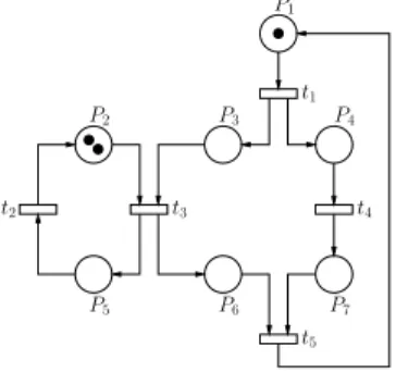
Fig. 2 presents an example of aGSPNmodel. Based on this model, we show our decomposition technique applied in three different approaches. For all the possible decomposition approaches, the demonstration in Section 4.2 can be used to obtain the equivalent tensor algebra representation automatically.

5.1 Decomposing by Places

Firstly, we analyse a quite naive approach, which is based on decomposing a

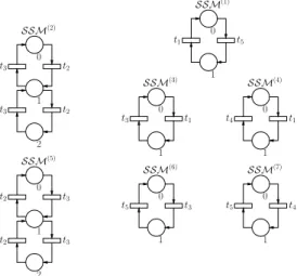
GSPN model by places. Each place has a maximum number of tokensK, and so we can view each place as aSSM withK+ 1 states. A decomposedGSPN model byplaces of Fig. 2 is presented in Fig. 3.

Each componentSSM(i)represents the possible states of placepiof aGSPN model. Note that places p2 and p5 in Fig. 2 are 2-bounded, i.e., there are no

P1 P2 P3 P4 t1 t2 t3 t4 P5 P6 P7 t5

SSM(1) SSM(3) _SSM(4) SSM(5) SSM(6) _SSM(7) t1 t5 t3 t3 t2 t2 t3 t1 t4 t1 t2 t2 t3 t3 t5 t3 t5 t4 SSM(2) 0 1 2 0 1 0 1 1 0 0 1 2 0 1 0 1

Fig. 3.Decomposed GSPN model byplaces

more than 2 tokens in each place in any marking M ∈ RS. Hence SSM(2) andSSM(5) have three places which represent the states (0, 1 and 2) of places

p2andp5 respectively. Analogously, placesp1,p3,p4,p6, andp7 are 1-bounded. So SSM(1), SSM(3), SSM(4), SSM(6), and SSM(7) have two states (0 and 1).

5.2 Decomposing by P-Invariants

Other decomposition of GSPN models is based onP-invariants. A P-invariant is composed of a set of places with constant token count. Fig. 4 presents a decomposed model of Fig. 2 using theP-invariants concept.

There are three minimal solutions ofσ given by equationσC = 0 (see Def-inition 8). So we can define three P-invariants to GSPN model of Fig. 2. PI1 has two places (p2 andp5),PI2 has three places (p1,p3 andp6), andPI3 also has three places (p1,p4and p7).

SSM(1) _SSM(2) _SSM(3) t2 t2 t3 t3 t1 t4 t5 t1 t3 t5

Each PIi corresponds to a componentSSM(i) of theGSPN model. So, in this example, we can decompose theGSPN model in three componentsSSM. It is important to note that, besides the transition superposition, there is a place superposition between componentsSSM(2) andSSM(3).

5.3 Decomposing as Superposed GSPN

Another possible approach to decompose aGSPN model is through transition superposition proposed by Donatelli [17]. Donatelli proposed the SGSPN for-malism in which components (subsystems) interact each other through transition superposition.

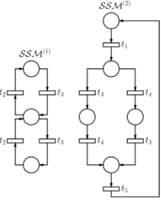
Example of Fig. 2 can be decomposed bySGSPN, since there is a transitiont3 which synchronizes two componentsGSPN. ComponentGSPN(1) is composed of two places (p2andp5), whereas componentGSPN(2)is composed of five places (p1, p3, p4, p6, and p7). Once defined the componentsGSPN(i), it is possible to obtain the equivalent components SSM(i). Fig. 5 presents the equivalent componentsSSM of theGSPN model (Fig. 2).

SSM(2) SSM(1) t2 t2 t3 t3 t3 t4 t4 t3 t5 t1

Fig. 5.Decomposed GSPN model bySGSPN

5.4 Decomposing Arbitrarily

It is also possible to decompose aGSPNmodel according to an arbitrarily chosen semantic. We can decompose the GSPN model of Fig. 2 as follows: markings of places p1,p2,p3, and p4, as well as markings of placesp5,p6, and p7. Hence componentSSM(1)is obtained from distinct markings of placesp1,p2,p3, and

p4 ofT RG, and componentSSM(2) is also obtained from distinct markings of placesp5, p6, andp7ofT RG.

Note that the decomposition choice may privilege some features of the tensor format which is important to the solution method. In some cases, it may be important to decompose a GSPN model considering: a large or small number of componentsSSM; a small number of reachable states; or even the difference between reachable and unreachable states.

5.5 Side Effect of Guards

The concept of guards in the GSPN formalism allows transition firing depen-dency according to the number of tokens in each place. Guards in GSPN are quite similar to functional elements in the SAN formalism [26, 18]. A natural decomposition among components GSPN of a GSPN model can be viewed through the use of guards. Therefore, guards in theGSPN models can allow to produce disconnected GSPN models, which have synchronization through the guards on theirs transitions.

As shown in Section 4.2, tensor format (Markovian Descriptor) of a decom-posedGSPN model uses generalized tensor sum and products.GTA operators in the Markovian descriptor are used to represent the functional rates of tran-sitions, but as long as there are no guards defined to trantran-sitions, they can be classical tensor products. Hence, guards on transitions are evaluated in Marko-vian Descriptor byGTA operators.

Another consequence of the use of guards is the possibility to define GSPN models with “disconnected parts”,i.e., models where there is not only a single net, but two or more nets with no arcs connecting them. In this case, there must be guards referring to places of other components in order to establish an interdependency (not a synchronization) among parts. The last example (Section 6.3) shows a net with disconnected parts and the use of guards to establish the interdependency.

6

Modeling Examples

We now present three modeling examples in order to present the approaches discussed in the previous section. The first one presents aStructured model, the second one describes aSimultaneous Synchronized Tasks model, whereas the last one shows aResource Sharing model.

6.1 Structured Model

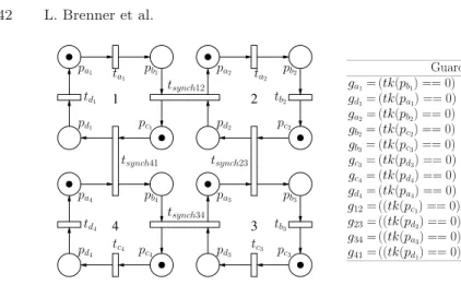
Fig. 6 presents an example of a Structured model composed of four submod-els. The submodeliis composed of four places (pai, pbi,pci,pdi) and two local transitions. There are also four synchronized transitions responsible for the syn-chronization of the submodels. It is important to observe that guards were chosen to define the possible firing sequence of transitions. This model was introduced by Miner [20].

In this model, the decomposition byplaces is rather catastrophic, since there is a correlation among marking of places. It results in a quite large product state space (65,536 states) for a rather small reachable state space (only 486 states). According to theSGSPNand P-invariants approaches, we have exactly the same decomposition and a more reasonable product state space (1,296 states). As a general conclusion one may discard the decomposition by places approach, but this is not really a fair conclusion, since this model is quite particular. Models

3 2 4 1 Guards ga1= (tk(pb1) == 0) gd1= (tk(pa1) == 0) ga2= (tk(pb2) == 0) gb2= (tk(pc2) == 0) gb3= (tk(pc3) == 0) gc3= (tk(pd3) == 0) gc4= (tk(pd4) == 0) gd4= (tk(pa4) == 0) g12= ((tk(pc1) == 0)&(tk(pa2) == 0)) g23= ((tk(pd2) == 0)&(tk(pb3) == 0)) g34= ((tk(pa3) == 0)&(tk(pc4) == 0)) g41= ((tk(pd1) == 0)&(tk(pb4) == 0)) pa1 _t a1 pb1 pa2 _t a2 pb2 td1 pd1 pd2 tsynch41 pa4 pb4 pa3 pb3 td4 pd4 tc4 _p d3 tc3 pc1 pc2 tsynch12 tsynch23 tsynch34 pc4 pc3 tb2 tb3

Fig. 6.Example of a structured model

with places with a larger bound (nets with more tokens) may be more interesting, as the next example will demonstrate.

6.2 Simultaneous Synchronized Tasks

Fig. 7 describes a Simultaneous Synchronized Tasks (SST) model in which five tasks are modeled. Such tasks have synchronization behavior among them, and those synchronization behaviors occur in different levels of the task execution.

t0 P₀ t₁ P₁ P₅ P₉ t₅ t₂ P₂ P₆ P₇ P₁₀ t3 t6 t9 P3 P₈ P₁₁ P₁₃ t₁₀ t₇ t₄ P₄ P₁₂ P₁₄ P16 t₁₁ P15 N t₈

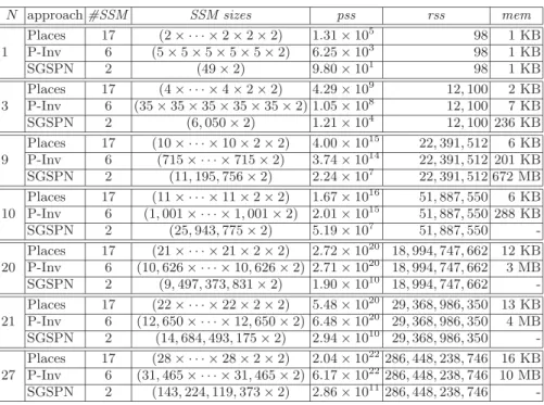
Table 1.Indices of decomposed SST models

N approach#SSM SSM sizes pss rss mem

1 Places 17 (2× · · · ×2×2×2) 1.31×105 98 1 KB P-Inv 6 (5×5×5×5×5×2) 6.25×103 98 1 KB SGSPN 2 (49×2) 9.80×101 98 1 KB 3 Places 17 (4× · · · ×4×2×2) 4.29×109 12,100 2 KB P-Inv 6 (35×35×35×35×35×2) 1.05×108 12,100 7 KB SGSPN 2 (6,050×2) 1.21×104 12,100 236 KB 9 Places 17 (10× · · · ×10×2×2) 4.00×1015 22,391,512 6 KB P-Inv 6 (715× · · · ×715×2) 3.74×1014 22,391,512 201 KB SGSPN 2 (11,195,756×2) 2.24×107 22,391,512 672 MB 10 Places 17 (11× · · · ×11×2×2) 1.67×1016 51,887,550 6 KB P-Inv 6 (1,001× · · · ×1,001×2) 2.01×1015 51,887,550 288 KB SGSPN 2 (25,943,775×2) 5.19×107 51,887,550 -20 Places 17 (21× · · · ×21×2×2) 2.72×1020 18,994,747,662 12 KB P-Inv 6 (10,626× · · · ×10,626×2) 2.71×1020 18,994,747,662 3 MB SGSPN 2 (9,497,373,831×2) 1.90×1010 18,994,747,662 -21 Places 17 (22× · · · ×22×2×2) 5.48×1020 29,368,986,350 13 KB P-Inv 6 (12,650× · · · ×12,650×2) 6.48×1020 29,368,986,350 4 MB SGSPN 2 (14,684,493,175×2) 2.94×1010 29,368,986,350 -27 Places 17 (28× · · · ×28×2×2) 2.04×1022286,448,238,746 16 KB P-Inv 6 (31,465× · · · ×31,465×2) 6.17×1022286,448,238,746 10 MB SGSPN 2 (143,224,119,373×2) 2.86×1011286,448,238,746

-Table 1 presents some indices to compare the decomposition alternatives. In this example, we use the following approaches: decomposing by Places (Sec-tion 5.1), decomposing by P-invariants (Sec(Sec-tion 5.2) and decomposing by Su-perposed GSPN (Section 5.3). N represents the number of tokens in place

P0. The number of SSM components, decomposed by all approaches, is indi-cated by#SSM.SSM sizes represents the number of states in each component SSM. Product State Space,Reachable State Space, and memory needs to store the Markovian Descriptor3 _{of the model are denoted by pss, rss, and mem} respectively.

The first important phenomenon to observe in Table 1 is the increasing gains of theP-invariantandPlacesapproaches achieved to models with largeNvalues. For small N values, there is much waste in the product state space that is not significant compared to the memory savings, specially for thePlaces approach. Regarding the comparison between SGSPN and P-invariant approaches, the model withN = 9 is a turning point, since the memory savings are already quite significant. In fact, larger models could not even be generated using theSGSPN decomposition. The relationship between product and reachable state space for

3 _{We do not take into account the memory needs to store neither the probability}

vector to compute solution, nor any special structure to represent the reachable state space.

decomposition based on P-invariants is considerably large, but we believe that an optimized solution for models with sparse reachable state space could take great advantage from this decomposition approach.

The second very impressive results taken from Table 1 is the very consistent gains of the Places approach. Even though the product state space waste is considerably large for smaller models (roughly one or two orders of magnitude), the difference between the product state space for the P-invariant and Places approaches becomes insignificant for theN = 20 model. Taking the model to its limits (N = 21 to 27) we observe an inversion, since thePlaces approach has a smaller product state space than theP-invariant approach.

6.3 Resource Sharing

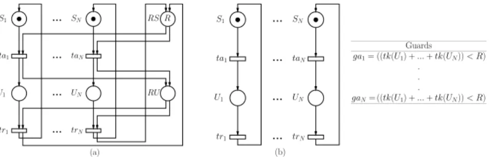
Fig. 8 (a) shows a traditional example of aResource Sharing (RS) model, which hasN process sharingRresources. Each processiis composed of two places:Si (sleeping) andUi(using). Tokens in placeRSrepresent the number of available resources, whereas they represent the number of using resources in place RU. Fig. 8 (b) is an equivalent model in which guards impose a restriction to the firing of each transitiontai.

... ... ... ... S₁ ta1 U1 tr₁ UN trN taN SN RS RU R (a) ... ... ... ... S1 ta1 U1 tr1 (b) trN UN taN SN Guards ga1= ((tk(U1) +...+tk(UN))< R) . . . gaN= ((tk(U1) +...+tk(UN))< R)

Fig. 8.(a) Resource Sharing without guards - (b) Resource Sharing with guards

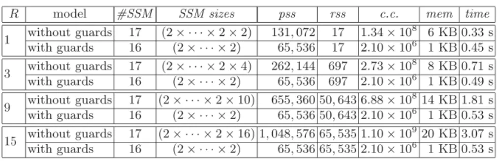
Table 2 shows some indices to compare the use of guards in a GSPNmodel producing, in this case, an equivalent disconnected model. The indices for the model of Fig. 8 (a) are shown in thewithout guardsrows, whereas indices for the model of Fig. 8 (b) are presented in thewith guardsrows.Rindicates the number of tokens in placeRS of Fig. 8 (a), as well as the number of available resources in the model of Fig. 8 (b). The computational cost (number of multiplications) to evaluate the product of a probability vector by the Markovian Descriptor4_, the memory needs and the CPU time to perform one single power iteraction are denoted byc.c.,mem andtime respectively. The numerical results for those

4 _{The vector-descriptor multiplication is the basic operation for most of the iterative}

Table 2.Indices of decomposed RS models (N= 16)

R model #SSM SSM sizes pss rss c.c. mem time

1 without guards 17 (2× · · · ×2×2) 131,072 17 1.34×10 8 _{6 KB 0.33 s} with guards 16 (2× · · · ×2) 65,536 17 2.10×106 1 KB 0.45 s 3 without guards 17 (2× · · · ×2×4) 262,144 697 2.73×10 8 _{8 KB 0.71 s} with guards 16 (2× · · · ×2) 65,536 697 2.10×106 1 KB 0.49 s 9 without guards 17 (2× · · · ×2×10) 655,360 50,643 6.88×10 8_{14 KB 1.81 s} with guards 16 (2× · · · ×2) 65,536 50,643 2.10×106 1 KB 0.53 s 15 without guards 17 (2× · · · ×2×16) 1,048,576 65,535 1.10×10 9_{20 KB 3.07 s} with guards 16 (2× · · · ×2) 65,536 65,535 2.10×106 1 KB 0.53 s

examples were obtained on a 2.8 GHz Pentium IV Xeon under Linux operating system with 2 GBytes of memory.

The results in Table 2 show the decomposition based on P-invariants, since decomposition based on SGSPN could only be applied to the without guards model. Observe thatSGSPN approach would result in exactly the same decom-position as P-invariants. The main conclusion observing this table is the absolute gains represented by the use of guards. It results in a model which has the same product state space independently from the number of resources, as well as the pss sizes are always smaller than those in the without guards models. It also has a smaller memory need and a more efficient solution (smaller computational cost).

It is a common mistake in some segments of the research community to assume that a model which requires functional evaluations (GTAoperators) has a bigger CPU time to perform vector-descriptor multiplication than equivalent models described only withCTA operators. In fact, such use of guards gives to thisGSPNmodel an efficiency as good as the one achieved by an equivalentSAN model [7]. Obviously, it happens due to theMarkovian Descriptorrepresentation usingGTA.

7

Conclusion

The main contribution of this paper is to follow up the pioneer works of Cia-rdo and Trivedi [14], Donatelli [17], and Miner [20]. Our starting point is the assumption that for really large (and therefore structured) models the main dif-ficulty is the storage of the infinitesimal generator. The solution techniques are rapidly evolving and many improvements, probably based on efficient parallel solutions, will soon enough be available. Using this assumption, we do believe that the tensor format based on Generalized Tensor Algebra has an important role to play.

For the moment, it benefits the Stochastic Automata Networks and it can also be applied to Generalized Stochastic Petri Nets. A natural future theoret-ical work is to expand those gains to other formalisms, such as PEPANETs [19]. A more immediate future work would be the integration of this

decompo-sition analysis to the solvers forSAN andGSPN (PEPS [6] and SMART [13] software tools respectively). It is easy to precompute the possible decomposi-tion with their memory and computadecomposi-tional costs. Therefore, the integradecomposi-tion of such precalculation may automatically suggest the best decomposition approach according to the amount of memory available.

Finally, we would like to conclude stating that the use of tensor based storage can still give very interesting results and allows the solution (which cannot be done without the storage) of larger and larger models.

References

1. M. Ajmone-Marsan, G. Balbo, G. Chiola, G. Conte, S. Donatelli, and G. Frances-chinis. An Introduction to Generalized Stochastic Petri Nets. Microelectronics and

Reliability, 31(4):699–725, 1991.

2. M. Ajmone-Marsan, G. Conte, and G. Balbo. A Class of Generalized Stochas-tic Petri Nets for the Performance Evaluation of Multiprocessor Systems. ACM

Transactions on Computer Systems, 2(2):93–122, 1984.

3. V. Amoia, G. De Micheli, and M. Santomauro. Computer-Oriented Formulation of Transition-Rate Matrices via Kronecker Algebra.IEEE Transactions on Reliability, R-30(2):123–132, 1981.

4. R. Bellman. Introduction to Matrix Analysis. McGraw-Hill, New York, 1960. 5. A. Benoit, L. Brenner, P. Fernandes, and B. Plateau. Aggregation of Stochastic

Automata Networks with replicas. Linear Algebra and its Applications, 386:111– 136, July 2004.

6. A. Benoit, L. Brenner, P. Fernandes, B. Plateau, and W. J. Stewart. The PEPS Software Tool. InComputer Performance Evaluation / TOOLS 2003, volume 2794 ofLNCS, pages 98–115, Urbana, IL, USA, 2003. Springer-Verlag Heidelberg. 7. L. Brenner, P. Fernandes, and A. Sales. The Need for and the Advantages of

Generalized Tensor Algebra for Kronecker Structured Representations.

Interna-tional Journal of Simulation: Systems, Science & Technology, 6(3-4):52–60,

Febru-ary 2005.

8. J. W. Brewer. Kronecker Products and Matrix Calculus in System Theory. IEEE

Transactions on Circuits and Systems, CAS-25(9):772–780, 1978.

9. P. Buchholz, G. Ciardo, S. Donatelli, and P. Kemper. Complexity of memory-efficient Kronecker operations with applications to the solution of Markov models.

INFORMS Journal on Computing, 13(3):203–222, 2000.

10. P. Buchholz and T. Dayar. Block SOR for Kronecker structured representations.

Linear Algebra and its Applications, 386:83–109, July 2004.

11. P. Buchholz and P. Kemper. Hierarchical reachability graph generation for Petri nets. Formal Methods in Systems Design, 21(3):281–315, 2002.

12. G. Ciardo, M. Forno, P. L. E. Grieco, and A. S. Miner. Comparing implicit rep-resentations of large CTMCs. In 4th International Conference on the Numerical

Solution of Markov Chains, pages 323–327, Urbana, IL, USA, September 2003.

13. G. Ciardo, R. L. Jones, A. S. Miner, and R. Siminiceanu. SMART: Stochastic Model Analyzer for Reliability and Timing. In Tools of Aachen 2001 Interna-tional Multiconference on Measurement, Modelling and Evaluation of

14. G. Ciardo and K. S. Trivedi. A Decomposition Approach for Stochastic Petri Nets Models. In Proceedings of the4th International Workshop Petri Nets and

Performance Models, pages 74–83, Melbourne, Australia, December 1991. IEEE

Computer Society.

15. M. Davio. Kronecker Products and Shuffle Algebra. IEEE Transactions on

Com-puters, C-30(2):116–125, 1981.

16. S. Donatelli. Superposed stochastic automata: a class of stochastic Petri nets with parallel solution and distributed state space. Performance Evaluation, 18:21–36, 1993.

17. S. Donatelli. Superposed generalized stochastic Petri nets: definition and efficient solution. In R. Valette, editor,Proceedings of the15thInternational Conference on

Applications and Theory of Petri Nets, pages 258–277. Springer-Verlag Heidelberg,

1994.

18. P. Fernandes, B. Plateau, and W. J. Stewart. Efficient descriptor - Vector multi-plication in Stochastic Automata Networks. Journal of the ACM, 45(3):381–414, 1998.

19. J. Hillston and L. Kloul. An Efficient Kronecker Representation for PEPA models. In L. de Alfaro and S. Gilmore, editors, Proceedings of the first joint

PAPM-PROBMIV Workshop), pages 120–135, Aachen, Germany, September 2001.

Springer-Verlag Heidelberg.

20. A. S. Miner. Data Structures for the Analysis of Large Structured Markov Models. PhD thesis, The College of William and Mary, Williamsburg, VA, 2000.

21. A. S. Miner. Efficient solution of GSPNs using Canonical Matrix Diagrams. In

9th International Workshop on Petri Nets and Performance Models (PNPM’01),

pages 101–110, Aachen, Germany, September 2001. IEEE Computer Society Press. 22. A. S. Miner and G. Ciardo. Efficient Reachability Set Generation and Storage Using Decision Diagrams. In Proceedings of the 20th International Conference

on Applications and Theory of Petri Nets, volume 1639 of LNCS, pages 6–25,

Williamsburg, VA, USA, June 1999. Springer-Verlag Heidelberg.

23. A. S. Miner, G. Ciardo, and S. Donatelli. Using the exact state space of a Markov model to compute approximate stationary measures. In Proceedings of the 2000 ACM SIGMETRICS Conference on Measurements and Modeling of Computer Sys-tems, pages 207–216, Santa Clara, California, USA, June 2000. ACM Press. 24. T. Murata. Petri nets: Properties, analysis and applications. Proceedings of the

IEEE, 77(4):541–580, April 1989.

25. B. Plateau. On the stochastic structure of parallelism and synchronization models for distributed algorithms. InProceedings of the 1985 ACM SIGMETRICS

confer-ence on Measurements and Modeling of Computer Systems, pages 147–154, Austin,

Texas, USA, 1985. ACM Press.

26. B. Plateau and K. Atif. Stochastic Automata Networks for modelling parallel systems. IEEE Transactions on Software Engineering, 17(10):1093–1108, 1991. 27. W. Reisig. Petri nets: an introduction. Springer-Verlag Heidelberg, 1985. 28. W. J. Stewart.Introduction to the numerical solution of Markov chains. Princeton