Manuscript version: Author’s Accepted Manuscript
The version presented in WRAP is the author’s accepted manuscript and may differ from the published version or Version of Record.
Persistent WRAP URL:
http://wrap.warwick.ac.uk/119064
How to cite:
Please refer to published version for the most recent bibliographic citation information. If a published version is known of, the repository item page linked to above, will contain details on accessing it.
Copyright and reuse:
The Warwick Research Archive Portal (WRAP) makes this work by researchers of the University of Warwick available open access under the following conditions.
Copyright © and all moral rights to the version of the paper presented here belong to the individual author(s) and/or other copyright owners. To the extent reasonable and
practicable the material made available in WRAP has been checked for eligibility before being made available.
Copies of full items can be used for personal research or study, educational, or not-for-profit purposes without prior permission or charge. Provided that the authors, title and full
bibliographic details are credited, a hyperlink and/or URL is given for the original metadata page and the content is not changed in any way.
Publisher’s statement:
Please refer to the repository item page, publisher’s statement section, for further information.
Did Austerity Cause Brexit?
⇤
Thiemo Fetzer
June 6, 2019
Abstract
This paper documents a significant association between the exposure of an individual or area to the UK government’s austerity-induced welfare reforms begun in 2010, and the following: the subsequent rise in support for the UK Independence Party, an important correlate of Leave support in the 2016 UK referendum on European Union membership; broader individual-level mea-sures of political dissatisfaction; and direct meamea-sures of support for Leave. Leveraging data from all UK electoral contests since 2000, along with detailed, individual-level panel data, the findings suggest that the EU referendum could have resulted in a Remain victory had it not been for austerity.
Keywords: PoliticalEconomy, Austerity, Globalization, Voting, EU
JEL Classification: H2,H3,H5, P16, D72
1 Introduction
Much of the recent rise of populism in the West has been attributed to a politi-cal backlash against globalization. A host of papers suggest that the distributional effects of globalization may causally explain the electoral success of populists (
Au-tor et al., 2016; Colantone and Stanig, 2018; Dippel et al., 2015). Other factors,
such as immigration and, in particular, the free movement of labor within the Eu-ropean Union (EU), may have similar distributional effects (Ottaviano and Peri,
2012;Dustmann et al.,2013), such factors feature prominently in populist rhetoric
as well. Globalization, by creating winners and losers, puts specific emphasis on the role of the welfare state (Stolper and Samuelson, 1941; Rodrik, 2000; Stiglitz,
2002). While a functioning welfare state can compensate the globalization’s losers
(Antras et al., 2016), welfare cuts may do the opposite. This paper provides
evi-dence that, at least in the context of the UK, the austerity-induced withdrawal of the welfare state since 2010 is an important driver to understand both how pres-sures to hold an EU referendum built up, and why the Leave side won.
I proceed in two steps. Using novel data on the universe of all elections held in the UK between 2000 and 2015, I present a set of observations that highlight how the political landscape changed in the UK in the period from 2010 to 2015 immediately prior to the referendum. I focus on the electoral performance of the UK Independence Party (UKIP). UKIP, established in the late 1990s, was prior to 2016, the only main party in the UK with the explicit goal of leaving the EU. Due to the tight correlation between UKIP vote shares and an area’s support for Leave
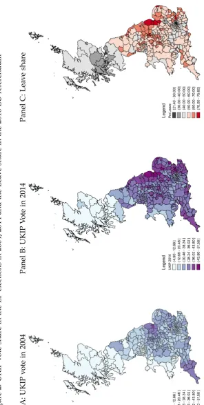
(seeBecker et al.,2017and FigureA1), UKIP’s evolution is an important window
into understanding the buildup of Leave sentiment. Exploiting high-frequency annual election data, I show that the EU referendum was precipitated by a signif-icant expansion in electoral support for UKIP in places with weak socioeconomic fundamentals. For instance, regions with a larger baseline share of residents in “routine jobs” with a larger share of “low-educated” residents, and with higher baseline employment shares in retail and manufacturing all experience an increase in support for UKIP,yet only after 2010.
-welfare spending per person fell by 23.4 percent in real terms between 2010 and 2015. Across districts, the extent of the cuts was widely variable, ranging from 46.3 percent to 6.2 percent, with the sharpest reductions in the poorest areas (Innes and
Tetlow, 2015). Using data from government estimates on the expected intensity
of specific welfare cuts across districts, I show that support for UKIP started to grow in areas with significant exposure to specific benefit cuts after these became effective. As a further plausibility check, I use the austerity shock to estimate mul-tiplier effects on local GDP; this yields estimates that compare well with those in the literature (Ilzetzki et al.,2013).
The austerity-induced increase in support for UKIP is not negligible and sug-gests that the tight 2016 EU referendum could have well resulted in a victory for Remain had it not been for austerity. (Leave won by a margin of 3.8 percentage points) The point estimates suggest that UKIP vote shares increased by between 3.5 to 11.9 percentage points due to austerity. Given the tight link between UKIP vote shares and an area’s support for Leave, simple back-of-the-envelope calculations suggest that Leave support in 2016 could have been easily at least 6 percentage points lower. Because, as this paper shows, support for UKIP is likely to under-state the overall impact austerity had on Leave sentiment, the results suggest that without austerity, Remain would likely have won the EU referendum.
populations (for example, households living in social housing judged to have a “spare bedroom”). Further, for a set of benefit reforms I can document auxiliary effects directly along relevant margins (for example, households living in social rented housing with a “spare bedroom” avoiding benefit cuts by moving to smaller accommodation). While UKIP gains among those exposed to cuts, support for the Conservative Party that brought about the cuts goes down. This suggests that there are political costs to austerity - a notion for which there is limited evidence in the literature (Arias and Stasavage,2016;Alesina et al.,2011,1998).
Lastly, while an in-depth exploration of the underlying economic reasons of why individuals become reliant on the welfare state (and thus, exposed to aus-terity) goes beyond this paper, I provide some suggestive evidence indicating that shocks and economic trends that contribute to the skill divide in labor markets are likely particularly relevant. I show that, consistent with the literature
document-ing growdocument-ing polarization in labor markets (Card and DiNardo, 2002; Lemieux,
2006;Goos et al.,2014), in the past 15 years UK labor incomes diverged along the
human-capital divide. Against this backdrop, the UK welfare state was responsive, providing growing transfers to those who, in relative terms, were increasingly left behind. This came to an abrupt halt from 2010, as the welfare reforms started to bite, marking the onset of the populist backlash. While a host of economic mechanisms which may contribute to the growing skill bias in the economy1, the
patterns are very consistent with this paper’s central argument, which suggests that austerity was key to activating these existing grievances, and to producing the sentiment that ultimately culminated in the Brexit vote.
This paper is related to several strands in the literature. The paper highlights that, at least in the UK context, economic drivers are a non-negligible factor to understand the rise of populism. This lies in contrast with research that traces the origins of the populist wave to a latent cultural drift within Western societies with work such asFukuyama(2018),Mutz(2018) and Norris and Inglehart(2019) mostly suggesting that economic factors are less relevant. In research similar to
1For example trade integration and offshoring (Autor et al.,2013;Scheve and Slaughter,2004),
that of this paper, B´o et al. (2018) carefully trace the economic origins of the re-cent rise in the populist Swedish Democrats to policy-induced economic losses exacerbating grievances between labor market “outsiders” and “insiders.” They suggest that economic pressures may make people more receptive toward mes-sages emphasizing the fiscal costs of immigration; the effect may be an indirect one, as they suggest that the growth in anti-immigration attitudes appears second order compared to the overall growth of distrust among the economic distressed.
Guiso et al. (2018) study the supply- and demand-side of populism. After
ac-counting for turnout, they suggest that economic insecurity is an important driver of demand for populist policies. Also in Sweden, Dehdari (2017) links economic distress to support for right-wing parties, whileAlgan et al.(2017) document that in areas and among individuals more exposed to economic shocks in the wake of the financial crisis, support for populist parties and distrust in political institutions grew. Trade integration with low-income countries may similarly have contributed to the buildup of economic grievances; these grievances have been suggested as an important causal factor behind the surge in populism (Autor et al.,2016;Colantone
and Stanig,2018;Che et al.,2017;Dippel et al.,2015).2 While labor market
dynam-ics are important in contributing to the growing reliance on the welfare state, the results presented here are not confounded by labor market shocks; rather, they capture genuine effects due to changes in the UK’s welfare system.
Another related literature links the recent rise in populism to various forms of immigration, which typically features strongly in populist rhetoric. While the effects may depend on the underlying type of immigration (e.g. legal or illegal immigration, refugee movements), the literature broadly documents, with a few exceptions, that support for right-wing platforms increases in areas affected by mi-gration (seeMayda et al.,2018for the US,Dustmann et al.,2018 in Denmark and
Halla et al., 2017 in Austria).3 While anti-immigration rhetoric featured strongly
2This builds on a rich literature studying the distributional effects of globalzation (Revenga,
1992;Autor et al.,2013;Grossman and Rossi-Hansberg,2008;Scheve and Slaughter,2001b).
3Scheve and Slaughter(2001a);Hainmueller and Hopkins (2014) study preferences over
im-migration policy in the United States. A rich literature studies the economic effects of im-migration:
in the 2016 EU referendum campaign, the results presented here suggest that sup-port for UKIP can be associated to an individuals’ exposure to welfare reforms producing distinct grievances. By documenting that populist voting in the UK can be linked to exposure to austerity through welfare reforms, this paper relates to a growing literature studying the interactions between political preferences and austerity, or fiscal policy more broadly (Alesina et al.,2011,1998). A paper closely related to this one isGalofr´e-Vil`a et al.(2017), who link the rise of the Nazi Party in the 1930s to an area’s exposure to austerity. Also related is the work ofPonticelli
and Voth(2017), who find a positive correlation between austerity and popular
un-rest more broadly. Arias and Stasavage(2016) find no evidence of a political cost to austerity; their findings are similar to those ofAlesina et al.(2011). This paper is able to tackle many plausible identification concerns that arise when working with low-frequency election results data, by turning to rich high-frequency indi-vidual level panel data. The paper presents evidence on a range of further margins, which indicate that exposure to welfare reforms produced tangible grievances that contributed to a consequential political effect: Brexit.
Lastly, the paper naturally relates to a growing literature on Brexit. Most of this work is purely cross sectional. By contrast, this paper comprehensively adds a time dimension.4 Colantone and Stanig (2018), following the seminal paper by Autor
et al.(2013), find compelling evidence suggesting that Leave support was distinctly
higher in areas of the UK most exposed to import competition from low-income countries. This paper qualifies these findings, suggesting that post-2010 austerity, by cutting transfer payments to globalization’s likely losers, is an important factor that can explain the timing of the UK’s populist revolt. Further, the paper suggests that the economic origins of exposure to the welfare state (and, hence, to austerity) likely go beyond what can be explained by trade integration alone. Turning to the consequences of Brexit,Born et al.(2018), using a synthetic control approach, estimate a cumulative Brexit-induced output loss of£19.3 billion, accrued between the EU referendum and the end of the 2017 calendar year. Given that the fiscal
4A rich descriptive correlational and purely cross-sectional literature emerged since the Leave
vote (seeHobolt,2016;Goodwin and Heath,2016;Becker et al.,2017), while (populist) campaigning and social media around the EU referendum are studied in a few papers (Gorodnichenko et al.,
savings of the austerity measures studied in this paper were projected to be around £18.9 billion per year, this suggests that the economic costs of Brexit are likely already higher than the austerity-induced fiscal savings that this paper argues significantly contributed to Brexit. More broadly,Dhingra et al.(2017) discuss the cost (and benefits) of the UK leaving the EU, whileBreinlich et al.(2017) document the welfare losses due to inflation following the Brexit-induced drop in the value of the pound.
The rest of the paper proceeds as follows: Section2, discusses the context and
the main data. Section 3 provides motivating evidence. Section 4 studies the
impact of austerity at the district level, while Section 5 turns to individual level data. Section6concludes.
2 Context and data
2.1 UK Politics, the EU, and the EU referendum
The UK joined the European Economic Community (EEC), the precursor of the EU in 1973, and held its first ”in or out” referendum just two-and-a-half years later following the Labour Party’s 1974 pledge to renegotiate the terms of British mem-bership of the EEC, and to consult the public in a referendum on whether Britain should stay in the EEC on the new terms. The referendum on 5 June 1975 asked the electorate: “Do you think that the UK should stay in the European Commu-nity (the Common Market)?”. The referendum resulted in a decisive victory for remain with a victory margin of 34.5 percent. Since the 1975 Referendum, the EEC has evolved into the central pillar of what became the European Union with the Maastricht Treaty of 1993. Further steps to European integration were formalized through the treaties of Amsterdam in 1997, Nice in 2001, and Lisbon in 2009.
and Whitaker, 2013). UKIP gained traction over time, attracting defectors mainly from the Conservative Party, and developing a footprint in local, European and Westminster elections. Earlier cross-sectional work suggests that UKIP drew its supporters from two pools of voters: 1) more affluent middle-class “strategic de-fectors” from the Conservatives who identify with UKIP’s Euroskeptic platform, and, later, 2) economically struggling, working-class voters with traditional Labour Party backgrounds (see Ford et al., 2012). Because electoral support for UKIP is tightly related with Leave support in 2016, it provides a good proxy variable to pick up broader “Leave sentiment,” which, as I will show, encapsulates broader measures of disaffection as well.
UKIP was seen as a threat to the Conservatives leading the party to adopt anti-EU stances: In March 2009, the Conservatives left the centre-right block in the European Parliament to join a group of right-wing parties, while the 2010 Con-servative manifesto set out “to bring back key powers over legal rights, criminal justice and social and employment legislation to the UK.” In the run-up to the 2015 general election, UK Prime Minister David Cameron pledged to hold an EU referendum by the end of 2017 if the Conservative Party were to win the election. Reports suggest that Cameron never expected to find himself in circumstances necessitating action on his pledge as he, and most polls, predicted another hung parliament and a continuation of the coalition with the pro-EU Liberal Democrats.5
Yet, electoral gains for UKIP in England and the SNP in Scotland split the oppo-sition votes, resulting in a surprise outright election win for the Conservatives. After a round of negotiations with the EU, the EU referendum was called, with Cameron campaigning for Remain in 2016.
The official Leave campaign and UKIP’s own Leave campaign used an aggres-sive populist campaign that likely would have resonated well in areas most af-fected by austerity. Throughout, the Leave campaign wrongly claimed that the “UK sends£350 million to the EU every single week”.6 The correct figure is£181
5The Guardian, Cameron did not think EU referendum would happen, https://goo.gl/
Vsmgnt, accessed 03.03.2019.
6The following inline quotes are from advertisements run by the Vote Leave campaign. These
million, amounting to 1.2 percent of overall UK government spending.7 The
cam-paign suggested that the UK’s contribution to the EU budget could be used to support the National Health Service (NHS), which faced pressures that the cam-paign in turn blamed on immigration. The camcam-paign highlighted that “layoffs and hospital closures continue throughout the UK” because “money is running out,” stoking fears about whether “your local NHS [could] survive.” The campaign sug-gested that leaving the EU was without risks as the UK would hold all the cards in any subsequent negotiations with the EU. It suggested that the UK could re-tain the benefits of EU membership without meeting any of its obligations, and it implied that a windfall profit would result from leaving the EU “to spend on OUR PRIORITIES and NOT THEIRS.” Similarly, the campaign suggested that im-migration is to blame for cuts in the UK health care system as “local hospitals are shutting down across the UK because of pressures from EU immigration policies”. The campaign further claimed that “the EU acts overwhelmingly in the interests of big business and against the interests of workers,” and suggested that remain-ing in the EU would erode workers’ rights. Lastly, the campaign suggested that UK public money was wasted by supporting luxurious lifestyles of “corrupt” EU bureaucrats; it contended that “EU officials wasted thousands of pounds on elite chauffeur services and prestige cars.” It is not inconceivable that this type of cam-paigning was particularly effective in areas and among people most affected by
austerity.8 After a 10 week campaign period, Leave narrowly won the referendum
with 51.9% of the votes on 23. June 2016.
2.2 Measuring Leave sentiment
Throughout this paper, the electoral performance or expressions of support for UKIP is a key outcome variable. I next describe both the data on the electoral 7Office of National Statistics, The UK contribution to the EU budget,https://goo.gl/nsVuaD,
accessed 03.03.2019.
8UKIP’s 2015 manifesto was not campaigning on a very distinct anti-austerity platform
performance of UKIP across elections, and the individual-level panel data.9
Election data I leverage data from the population of electoral contests between
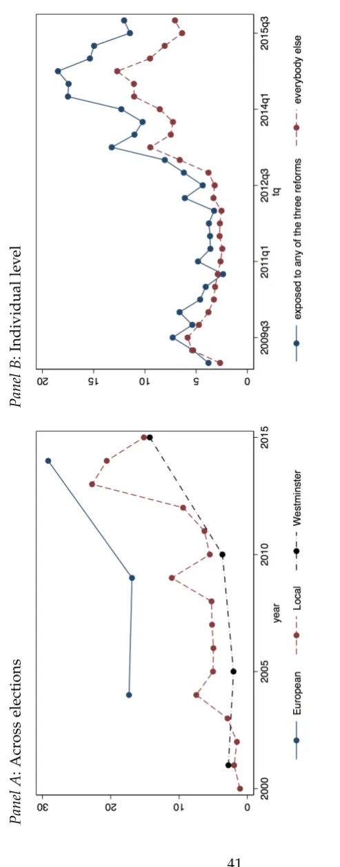
2000 to 2015, drawing on data from Westminster, European, and local council elections in this time frame, as well as from the 2016 EU referendum. The per-formances of UKIP across the different types of electoral contests over time are
presented in the left panel of Figure 1. Support for UKIP surged significantly
after 2010 across all election types, yet, the overall levels of support for UKIP are different, which is due to the different electoral systems and due to the way election results are reported. Westminster elections are conducted using a first-past-the-post (FPTP) electoral system, which results in voters casting their votes strategically, favoring large parties. As a result, UKIP, like most other small par-ties, has performed quite poorly, with its vote share being well below 10 percent prior to 2010. Yet, in 2015 UKIP came in third, winning 12.6 percent of the popu-lar vote, while still only winning a single seat (which was held by a Conservative Party member who had defected to UKIP), highlighting the distortions introduced by FPTP.10 Constructing consistent measures of an area’s population’s political
preferences across Westminster elections is difficult due to regular constituency boundary changes. Bearing in mind these caveats, I harmonize the results across elections to the 2001 constituency boundaries using detailed ward-level shapefiles together with 2001 population figures. The resulting data set is a balanced panel of 570 harmonized constituencies in which I measure UKIP’s vote share; I assign an area with a zero if UKIP did not field a candidate there.
I also leverage data from the European Parliamentary (EP) Elections held in 2004, 2009, and 2014. These elections report results at the local authority district level. Importantly, they essentially use proportional representation to allocate the British seats in the European Parliament. Not surprisingly, as strategic voting con-cerns do not weigh in, UKIP has significantly higher vote shares, increasing from 15.6 percent in 2004 to 26.6 percent in 2014. The extent and the spatial distribution
9Summary statistics of the main variables are provided in Appendix TableA1.
10A further distortion may be introduced since not all parties field candidates in each
of UKIP support base across EP elections changed significantly between 2004 and 2014, as Figure2 illustrates. UKIP gains since 2004 are most concentrated in the coastal regions, Wales, and parts of the industrial areas of the Midlands. Panel C presents the spatial distribution of the 2016 EU Leave vote share, for which the official counting areas were also the 380 local authority districts; the map high-lights the tight relationship between an areas’ support for UKIP and support for the Leave already alluded to earlier. While EP elections use proportional represen-tation, and are thus able to pick up protest voting quite well, EP elections usually have low turnout. Further, EP and Westminster elections happen only infrequently, which may limit the statistical power of analysis exploiting time-varying shocks.
To navigate the issue of the low-frequency nature of EP and Westminster elec-tions, I also make use of local council election data for England and Wales since 2000. Local elections have an appealing feature in that, rather than happening uni-formly across the UK every four years such elections may take place in any given year across the UK due to the rotating fashion by which councillors are elected.11
The left panel of Figure 1highlights that across local elections, UKIP’s vote share hovered between Westminster election performance (as lower bound) and Euro-pean election performance (as upper bound), ranging from between 5 percent and 12 percent in the 2004-2009 period, and peaking at 22.7 percent in 2013. Yet, the figures are likely downward biased because most local elections are conducted at the local ward level, while election results are collated at the level of the local au-thority district.12 This implies that if UKIP does not field candidates in each of the
races at the ward level, UKIP’s vote shares are mechanically downward biased as wards that were not contested mechanically contribute zero votes.13
While each of the different types of election results data has its own advantages and disadvantages, the results focusing on election outcomes are robust across election types. I next detail the individual-level panel data, which allow for sharper empirical designs and finer outcome measurement.
11Terms last for four years, and most councils hold elections by “thirds” with a third of the seats
up for election each year, and with no election held one year. See appendixB.1for more details.
Individual-level panel data This paper leverages a newly constructed individual-level panel data set, making use of the USOC panel study with approximately 40,000 households contributing across the UK. Participating households are vis-ited, on average, every year. Interviews are carried out face to face in respondents’ homes by trained interviewers or through a self-completed online survey. Respon-dents are coded based on the residence at the district-level and in this paper, I use data from the first eight waves covering the years from 2009 to 2016. Given the gradual data collection, I can construct a quarterly individual-level unbalanced panel.
The survey instruments used across waves are quite harmonized. In particular, each survey wave includes an instrument eliciting respondents’ and households’ sources of income and employment status. Further, most survey waves include a module to elicit political preferences. Respondents are first asked “whether they see themselves a supporter of a specific political party” or “whether they are closer to a political party compared to another.” If neither of these questions is success-ful in eliciting a response of a party name, the remainder of the respondents are asked which party they would vote for if a general election were held tomorrow. The resulting answers are coded as dummy variable if respondent expresses sup-port for UKIP (or any of the other parties).14 Panel B of Figure1presents the share
of respondents expressing support for UKIP over time. The plot highlights that support for UKIP surged from around 2013 onward, and remained distinctly high among individuals directly exposed to any of the three welfare reforms studied in detail in Section 5. In addition to asking questions about political party pref-erences, survey waves two, three and six included further measures of of broader dissatisfaction or discontent, asking questions of individual’s perceived political influence (whether individuals think their vote makes a difference), the extent to which they think that “public officials do not care” or that they have “no say in what government does.” I use these measures as further outcome variables capturing broader discontent and anti-establishment sentiment. These sentiments
14Hence, for a significant share of respondents, preferences are elicited without election framing;
are strongly associated with Leave preferences and also strongly increase among those exposed to welfare reforms. Further, as I later discuss in detail, the data al-low me to study other adjustment margins directly relevant to some of the reforms studied. Lastly, the most recent USOC wave 8 actually asks the EU referendum question, providing an additional, immediately relevant outcome measure, which I will link with the empirical analysis of support for UKIP and the measures of broader discontent.
I next present a range of stylized facts used to motivate the subsequent analysis.
3 Where (and when) did UKIP start to grow?
I first present a range of stylized facts, which highlight that UKIP-support dis-tinctly grew in areas with weak socioeconomic fundamentals, but only after 2010.
3.1 Empirical specification
Using data from the local, Westminster and EP elections, I estimate the follow-ing regression:
yi,r,t =ai+br,t+
Â
t6=2010ht⇥Yeart⇥Xi,baseline+ei,r,t (1)
where yirt denotes UKIP vote shares in council, Westminster and EP elections.
The fixed effect ai absorbs any time-invariant differences in political preferences
or sentiment across districts.15 Region-by-time fixed effects b
rt capture non-linear
time trends specific to each of the eleven regions across the UK. The main coeffi-cients of interest are the interaction terms between (fixed) baseline socio-economic characteristic Xi,baseline and a set of year fixed effects. I plot out the estimated
coefficients ˆhtover time relative to 2010 as the reference year (2009 for the EP
elec-tions) to capture how UKIP differentially gained support over time as a function of Xi,baseline. Throughout the paper, standard errors are clustered at the district level
(constituency level for the Westminster election analysis).16
15Local Council election results, similar to EP elections, are reported at the district level; the
Westminster election results data is presented at the harmonized 2001 constituency level.
16Districts are the main meaningful subnational administrative unit in the UK. Results are robust
I focus on four main characteristics Xi,baseline that stand out due to their
promi-nence in the cross-sectional analysis of the Leave vote and their relevance to the wider literature: the share of the 2001 resident population with no formal qualifica-tions, the share working in routine jobs, and the working-age resident population shares working in the manufacturing and retail sectors.17
3.2 Results
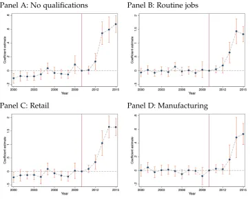
I discuss results for the local elections presented in Figure3in more detail.18
Human capital Panel A of Figure3focuses on a baseline proxy measure of area’s
population’s human capital. The results suggest that support for UKIP gradually
trends up as a function of the share of the resident population with low educational attainment. The correlation between support for UKIP and the measure of low human capital only becomes sharply strongerafter 2010.
Routine jobs In Panel B of Figure 3, I present results when studying how the
degree of correlation between support for UKIP in local elections and the share of
an area’s working-age population employed in routine jobs as per the Census
so-cioeconomic statusclassification. Prior to 2010, support for UKIP is not statistically associated with the share working in routine jobs. Since 2010, this correlation be-comes sharply stronger, which can account for, on average, 7.5 (or 6.7) percentage points of the increase increase in UKIP vote shares in local elections since 2010 (in EP elections between 2009 and 2014).
Economic structure Lastly, panels C and D of Figure 3 zoom in on measures
of a district’slocal economic structure, focusing on employment shares in retail and manufacturing sectors. The latter is of particular interest due to the manufacturing sector’s exposure to trade integration. The retail sector is represented all across the country, and the sector is, for the bulk of jobs, not directly subject to global trade exposure; at the same time, however, it provides relatively low-quality jobs, and
17AppendixC.1shows that patterns presented here are robust to alternative fixed effects,
dif-ferent sample cuts and broader or more refined baseline measures. Further, in appendix C.2, I document that the growth of UKIP is mostly at the expense of the Conservative party.
18Appendix FigureC1and FigureC2highlight that I obtain very similar results studying UKIP’s
is likely indirectly affected by contractions in consumer spending. Areas with larger employment shares in retail and manufacturing saw significant increases in electoral support for UKIPafter 2010. As we will see, these sectors are dispropor-tionately affected by the contraction in local area incomes due to austerity.
Discussion The observation that UKIP, after 2010, starts to thrive distinctly in
areas characterized by low educational attainment, and a significant share of the population working in routine jobs or in manufacturing or retail suggests that the
underlying causal drivers of the EU referendum may gobeyond what is currently
known. The extent of knowledge on this issue has been limited because most papers thus far have studied the topic using cross-sectional data.19 A central
ques-tion is why the structure of support for UKIP only changed so rapidly after 2010. The next sections presents evidence on how austerity is the likely causal factor explaining these trends, starting with aggregate district-level evidence in Section4
and then moving to evidence from individual-level data in Section5.
4 Austerity as activating factor?
I next present evidence from aggregate data suggesting that austerity measures are likely factors behind the shift toward UKIP.
4.1 Aggregate trends in fiscal spending
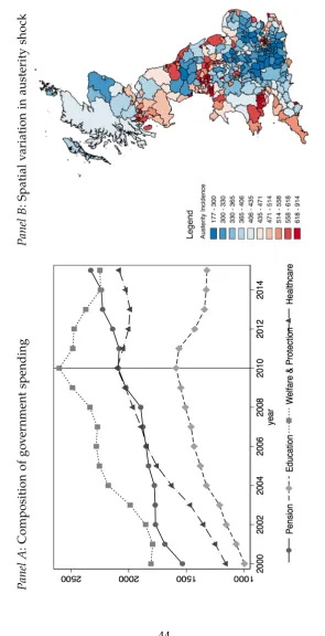
In the wake of the financial crisis, the Conservative-led coalition government that came to power after the May 2010 General Election brought forward wide-ranging austerity measures to reign in public-sector deficits. The government cut spending across all levels of government. Panel A of Figure4suggests that, start-ing in 2011, spendstart-ing for welfare and social protection dropped significantly, de-clining by 16 percent in real terms, falling to levels that had last been seen in the early 2000s. Spending on healthcare, which was spared direct cuts, flatlined. Yet the rapidly aging population added pressures on health care services. Further, spending on education contracted by 19 percent in real terms, while expenses for 19Colantone and Stanig (2018) suggest that import-competition may be an important causal
pensions steadily increased, suggesting a significant shift in the composition of government spending. The Conservative-led government used three methods to cut spending. First, the initial wave taking immediate effect with the announce-ment of the autumn budget in 2010 cut budgets for day-to-day spending across
most Westminster departments.20 Local government funding fell significantly,
putting pressures on local councils to provide services, despite increasing demand due to population growth (Innes and Tetlow,2015). A second significant compo-nent took the form of nominal freezes. From 2011 to 2013, the government froze salaries of public-sector employees earning more than£21,000. Beginning in 2014, it capped public-sector wage growth at 1 percent. Similar freezes were introduced for most welfare benefits, resulting in cuts in real terms, as inflation averaged be-tween 2 and 4 percent throughout this period. In this paper, I focus on the third important component of austerity – the reform of the welfare state – which was set in motion through the Welfare Reform Act 2012.
4.2 Exposure of welfare cuts at the district level
I draw on data from Beatty and Fothergill(2013), who, using detailed data on the distribution of claimants across different types of benefits before reforms be-came effective, provide an estimate of the incidence of the different welfare cuts at the district level. Beatty and Fothergill (2013) consider 10 different measures, which, taken together, were expected to yield fiscal savings of up to£18.9 billion per year by 2015. The estimates of the intensity of exposure of an area to the welfare reforms are “deeply rooted in official statistics” drawing in “data from the Treasury’s own estimates of the projected savings, the government’s impact assess-ments, and benefit claimant data.”21 The exposure of an area to specific reforms is
measured as the financial loss per working age adult in a district and year. The ag-gregate figure masks a wide range of variation in the intensity of treatment, which is driven by the heterogeneity in the distribution of benefit claimants across the UK prior to the reforms. This variation is visually presented in Panel B of Figure
4. The overall projected financial loss per working adult varied between £914 in 20The Department for International Development and the Department for Health, which funds
the National Health Service (NHS), were spared cuts.
Blackpool and£177 in the City of London.
The measures with the largest effect were the reform of tax credits, changes to child benefit, and the capping of benefit increases to account for inflation to 1% per year. Tax credits are a means-tested transfer to households to top up low incomes; child benefit is an unconditional benefit paid out to families. The re-form of tax credits involved a faster withdrawal of the transfer payment as income grows, in addition to a host of changes to eligibility requirements. This complexity makes identifying the affected group in the population difficult because exposure depends on a rage of characteristics. In the case of child benefit, the main measure was to make the benefit means tested withdrawing child-benefit from better-off households with at least one earner with an annual pre-tax income above£50,000. According to the estimates from the Department of Works and Pensions, these three measures alone were expected to generate around£10 billion in savings per year by 2015. It is estimated that changes to tax credits and child benefit affected between 4.135 million to 6.980 million households, or roughly between 15-25 per-cent of the 27.2 million UK households. My paper demonstrates that these specific measures, while having small direct effect on individual households, had sizable indirect effects on the local economy.22 In the individual-level analysis, I focus on
three smaller welfare reforms – the abolishment of council tax benefit, the so-called “bedroom-tax” and the introduction of Personal Independence Payments replac-ing Disability Livreplac-ing allowance – about which I provide more detail later in Section
5. I first estimate the impact of the overall welfare-reform austerity measures on voting outcomes, incomes, and support for Leave.
4.3 Empirical strategy
I perform three related exercises. First, I estimate a difference-in-differences specification to study how support for UKIP distinctly grew after 2010 in areas more exposed to cuts across local, European and Westminster elections. I fur-ther explore an event study design similar to specification 1, where I replace the measure Xi,baseline with a measure the exposure of district i to welfare reform j,
22In total, the paper studies five measures in some detail. The other reforms are indirectly
Austerityi,j. Further, I study a specification allowing me to estimate local multipli-ers. The pooled difference-in-difference specification takes the following form:
yi,r,t= ai+br,t+g⇥1(Year> 2010)⇥Austerityi,j+ei,r,t (2)
The only difference compared to the earlierevent studiesspecification1 is that the treatment periods are pooled together. As we will see when studying the event studies as second exercise, this is likely to underestimate the specific impacts of some benefit cuts that only became effective starting 2013.
For the third exercise, the estimation of local multipliers, I obtained district-level data from the Office of National Statistics (ONS) on local area gross value added by sectors.23 I also estimate an event study to highlight that contractions
in district GDP due to austerity only occur after austerity takes effect. Lastly, I show that exposure to austerity, changes in support for UKIP and higher levels of support for Leave in 2016 in the cross section are tightly linked.
4.4 Results
I first discuss the pooled difference-in-difference results, before turning to the event studies and the estimates of the multipliers.
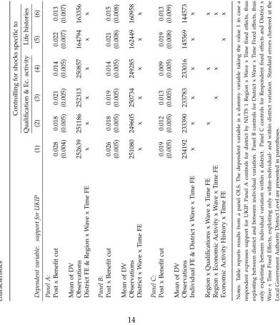
Pooled difference-in-difference The results from estimating specification 2 are
presented in Table 1. The rows explore UKIP’s electoral performance in local,
European and Westminster elections, while the columns explore the different wel-fare reformj-specific measures Austerityi,jtaken fromBeatty and Fothergill(2013). Column 1 studies the impact of the overall estimated impact of the reforms. The average anticipated financial loss per working-age adult was estimated to be£447.1. Given that the median household disposable income in the UK stands at just
around £27,300, this is a non-negligible amount. The point estimates indicate a
strong positive relationship between the austerity exposure and UKIP’s electoral performance. Computing the full in-sample distribution of point estimates implied by column (1) suggests that UKIP’s electoral performance increased, on average, by 6.5, 3.5, 3.8 percentage points across local, European or Westminster elections
respectively after 2010.
Columns 2-6 zoom in to a set of specific benefit cuts, in particular, changes to tax credit (TC) and child benefit (CB). For the former, I find sizable effects on support for UKIP, while for the latter the results are more mixed. This is due to the nature of the child benefit cut, which affected relatively well-off households. Other key welfare reforms (which are described in detail in Section5.2) - abolish-ing council tax benefit (CTB) and the disability livabolish-ing allowance (DLA), and the ”bedroom tax” (BTX) - almost exclusively affected low-income households. For these benefit cuts, I have reasonably sharp timings and eligibility rules that I can trace out in the individual-level data. Across most of these specific reforms, the aggregate election data suggest similar sized effects across Panels A - C.
At the bottom of Table 1, I provide some summary statistics on the size and
distribution of the cuts. For example, the bedroom tax explored in column (6) was expected to yield fiscal savings of just£10.81 per working-age adult; yet, the measure was much more concentrated, affecting an estimated 660,000 households. Further, I also provide the correlations between the share of working age house-holds affected by the reforms and the baseline district measures explored in section
3. This highlights non-negligible cross-correlations between an area’s exposure to austerity and these measures, indicating that indeed, benefit cuts were particu-larly concentrated in areas with significant resident shares with low qualifications or significant working-age adult populations working in routine jobs.
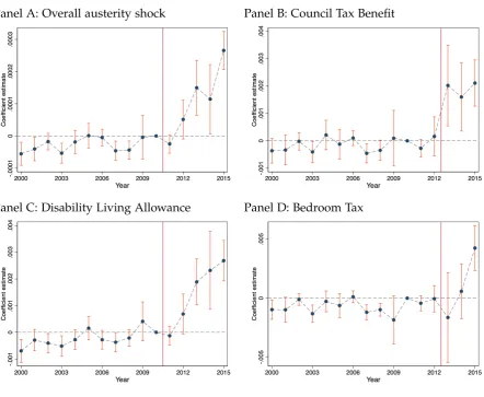
Event studies The pooled difference-in-difference analysis, by averaging the
co-efficient estimates after 2010, may underestimate the effect of austerity. Welfare cut measures, such as freezing of benefits, or changes in inflation indexing, com-pound over time, while others only become fully effective at a later date. This only affects the local election results, because for Westminster and EP elections, only a single election occurred in the time window between 2010 and 2015 before the referendum. Nevertheless, looking at Westminster and EP elections is still useful in terms of whether support for UKIP in more austerity-exposed areas followed similar trends prior to the time when the reforms took effect.
Wel-fare Reform Act 2012 and became effective with the start of the financial year in 2013, some measures, such as reforms to tax credits or nominal freezes had al-ready taken effect in 2011. In the event studies presented in Figure 5, I focus on the overall austerity exposure measure in Panel A, as well as three individual policies further detailed in the next section. Throughout, there is no evidence of systematic divergence before 2011 in a fashion that is correlated with exposure to austerity. Markedly, the timing is also quite consistent with the specific measures. The first effects appear in 2012 for the overall austerity measures in Panel A, which is significantly carried by the tax credit reforms taking effect from April 2011. The estimated coefficient for the year 2015 is, not surprisingly, larger compared to the pooled difference-in-difference estimates: the full distribution of implied ef-fect sizes across England and Wales suggests that the main austerity measure can explain an increase in support for UKIP of 11.9 percentage points by 2015.
Panels B - D focus on three reforms further detailed in the next section – the abolishment of council tax benefit, the so-called “bedroom-tax” and the introduc-tion of Personal Independence Payments replacing Disability Living allowance. There is no evidence of diverging pre-trends for any of these reforms. The timing of each of the effects is quite consistent with the times at which various measures (particularly for the abolishing of the council tax benefit) took hold.24
Local multipliers I estimate local spending multipliers as a further plausibility
check. The average local authority district was expected to lose£447.1 per working-age adult in transfer income, which should result in further indirect contractions of local incomes. I estimate these multiplier effects using data on local-area GDP estimates. The only difference from the main estimating equation is that the de-pendent variable now is the log value added per working-age adult by sector, while the independent variable is the overall austerity-exposure measure.
The results are presented in Appendix Table A3. The estimates suggest a sig-nificant negative relationship between austerity exposure and local GDP: for every 24Appendix FigureA2presents the same figures for Westminster elections. Appendix Figure
pound contraction in transfer income to working-age adults, local-area gross value added contracts by around 2.4 pounds. The multiplier effects are broadly carried by contractions in the distribution and retail sectors, as well as by the manufac-turing sector. The magnitude of the multipliers and the distribution across sectors are quite consistent with estimates in the wider literature (Ilzetzki et al.,2013).25
Austerity, UKIP, and Leave support in 2016 The previous results suggest that
austerity, at the aggregate level, is consistently and significantly associated with the steep rise in support for UKIP after individual austerity measures started to take effect. In turn, changes in support for UKIP across elections and the Leave vote are also tightly linked. In column (1) of Appendix Table A4, I highlight that areas exposed to austerity experience higher levels of support for Leave in 2016. Similarly, column (2) suggests that areas that see marked swings to UKIP across the three election types studied see higher levels of support for Leave in 2016. Across election types, the estimated coefficients suggest that a 1 percentage point larger swing to UKIP is associated with a 0.9 to 1.9 percentage point higher level of support for Leave in 2016. Column (3) further highlights that changes in sup-port for UKIP are tightly correlated with the district-level austerity exposure: after controlling for the swing to UKIP, the coefficient on the austerity measure shrinks markedly. This suggests that a lot of the variation that drives the correlation be-tween the austerity measure and the Leave vote share can, in fact, be captured by the change in support for UKIP.
I next turn to use these observations to provide back-of-the-envelope calcu-lations. The estimated effects of austerity and UKIP are sizable and substantially
meaningful: a victory for Remainin the 2016 EU referendum would have been much
more likely, had it not been for austerity. Taking the point estimates from column
(2) of Appendix Table A4, which links changes in support for UKIP with leave
support in 2016, I can obtain estimates of the potential impact that austerity had on support for leave. For European election, the previous analysis suggests that the austerity-induced increase in support for UKIP of around 3.5 percentage points may have translated into up to 3.5⇥1.9 = 6.7 percentage points higher levels of 25Appendix FigureA4shows that there are no pre-trends in local area gross value added across
support for Leave. For local elections, the full distribution of pooled difference-in-difference estimates suggested that the austerity exposure can account for, on aver-age, a 6.5 percentage point increase in support for UKIP. Taking the corresponding
point estimate from Appendix Table A4 suggests that leave support could have
been at least 6.5⇥0.9=5.9 percentage points lower. In the event studies for local elections, the analysis suggested that the increase in support for UKIP by 2015 that can be attributed to the main austerity measure is 11.9 percentage points. This would suggest that leave support in 2016 could have been up to 11.9⇥0.9= 10.7 percentage points lower. This implies that even conservative estimates would sug-gest that Remain would have won the EU referendum had it not been for austerity. Despite the consistency of results in terms of timing, magnitude, and election types, a range of concerns still make it difficult to interpret the results in a causal fashion. In particular, selection into benefit receipt could be endogenous to an area’s exposure to austerity. In addition, austerity may affect political preferences, and contribute to the buildup of Leave sentiment more broadly in ways that do not necessarily operate solely through changes in support for UKIP. Lastly, the ob-served changes in the election results could also reflect changes in composition of turnout (Guiso et al.,2018). To tackle these concerns, I next turn to an individual-level panel, which will allow me to get cleaner identification by tracking pools of individuals affected by specific welfare reforms over time.
5 Turning to individual level evidence
To overcome the issues highlighted when studying aggregate data, I turn to individual-level panel dataconstructed from the USOC study starting in 2009.
5.1 Capturing individual exposure to welfare cuts
received benefits of certain types and were thus, exposed to reforms.
The substantive concern for causal identification is selection. Individuals can be exposed to austerity in three different direct ways. First, individuals who have received benefits prior to the reform, may lose benefits altogether as a result of the reforms. Second, individuals who were not receiving benefits, due to a host of reasons (possibly related to austerity), may start receiving benefits from a now less generous welfare state. Third, individuals who had already and continuously received the same benefit prior to a reforms could see a reduction in the value or quality of the benefit. The main challenge is to distinguish those selection in (or out) of benefits as a result of the reforms vis-a-vis those whose personal situation changes for reasons unrelated to the welfare cuts.
5.2 Zooming in on individual benefit reforms
I next discuss three welfare reforms affecting roughly 10 percent of all UK households, for which I can tackle selection concerns rather well.
Council tax benefit abolishment (CTB) Council tax is a tax levied by local
coun-cils to pay for some public goods (e.g., waste collection). Up until April 2013, people earning low incomes could be exempted from paying council tax, or they could receive a rebate. The central government financed this benefit, but it was canceled without replacement starting with the new fiscal year in 2013. As a re-sult, an estimated 2.4 million households across the UK were asked to pay the full council tax for the first time starting in April 2013. The extent of council tax varies across the UK from council to council, but is usually at least around£1,000 annu-ally per household. I identify the population of individual households affected by this reform based on whether they consistently received council tax benefit at all the timesthey were surveyed prior to April 2013. This set of individuals was most likely affected by the abolishment of the council tax benefit and it is unlikely that results are conflated by endogenous selection. For the estimating equation to be explored in detail further below, I define a subset of treated individuals as:
Ti,CTB= 8 < :
1 received council tax benefit prior to April 2013
In addition, the USOC survey instrument consistently asked respondents whether they were “behind with their council tax payments,” allowing me to provide evi-dence on a direct reform impact margin.
Disability Living Allowance (DLA) Established in 1992, the Disability Living
Allowance (DLA) was a social security benefit paid to disabled individuals aged under 65 to help cover the cost of a personal care and/or mobility need due to a disability. It was a tax-free, non-means tested and non-contributory benefit with an estimated 3.2 million claimants across the UK by 2012. The Welfare Reform Act of 2012 lead to the replacement of DLA with a new system of benefits called Personal Independence Payments (PIP). PIP could be claimed by working-age claimants, and continues to be non-means tested; but involves regular work-capability as-sessments carried out by private contractors on behalf of the government.
The transfer to the new system caused significant public outcry. While only a relatively small share of DLA claimants lost their benefit following the reassess-ment, a change in the quality or conditionality of awards (by requiring regular work capability checks, for example) affected a non-negligible share of the 73 per-cent of recipients transitioned to PIP.26 The PIP roll out started from the 28th of
October, 2013 existing beneficiaries from DLA were gradually converted to PIP. Unfortunately, I do not know when individuals were converted from DLA to PIP, because these two benefits are lumped together in the benefit-receipt data.
To tackle selection, I focus on the subset of claimants who had a so-called indefinite award of DLA and, prior to the introduction of PIP, were not required to regularly reapply for the benefit. I code these lifetime recipients as treated from the fourth quarter 2013, when the roll-out of PIP started. For the empirical design, this set of affected individuals is identified as follows:
Ti,DLA = 8 < :
1 always received either DLA or PIP
0 else
Technically, all DLA recipients with a lifetime award should receive a similar mon-26Department of Works and Pensions (DWP), “Personal Independence Payment: Official
etary award through PIP. Nonetheless, the process and the requirement for assess-ment are said to have caused significant grievances.27
Bedroom tax (BTX) Housing benefit is a benefit paid to individuals on low
in-come living in social housing, as government-subsidized rental properties are called in the UK. As of April 2013, all current and future working-age tenants renting from a local authority, housing association, or other registered ”social land-lord” ceased to receive help that had previously been available to defray the costs of a spare room. This provision was also dubbed the “bedroom tax” in the popular press as it implied that a lot of working-age parents, whose children had moved out, found themselves living in accommodation with a spare bedroom. The rules allow one bedroom for each adult couple, for each single person over 16, for each two children of the same sex under 16 and for each two children of either sex un-der 10. Significant cuts were imposed on housing benefit for individual recipients who were found to have a spare room as per these definitions; financial support to pay rent fell by 14 percent for those found to have one spare bedroom, and by 25 percent for those found to have two or more.
I identify individuals who were most likely affected by the “bedroom tax” as follows. They mustcontinuously live in social housing (roughly 16.4 percent of the sample) and, they must have a spare bedroom as per the governments definition the most recent time they were surveyed before April 2013.28 This defines a simple
treatment indicator used in the various difference-in-difference estimations.
Ti,BTX = 8 < :
1 lives in social housing with excess bedroom(s) prior April 2013
0 else
27Anecdotes that generated outrage proliferated in the media. For example, articles
re-ported that wheelchair-bound claimants were asked to attend reassessment appointments in non-accessible facilities, and claimants with trisomy 21 (Down syndrom) were asked when they “caught it.” Further, there were concerns about the qualification of the staff of two private firms tasked with conducting the reassessments. The Independent, “Disability benefit assessors failing to meet Gov-ernment’s quality standards,”https://goo.gl/uX4yD5, accessed 23.06.2018.
28The requirement of living continuously in social housing is a conservative as some households
The bedroom tax was widely debated and affected more than 660,000 households across the country. To avoid financial losses, the government encouraged house-holds to “move to accommodation which better reflects the size and composition of their household.”29 I can directly measure two impact margins relevant to this
benefit cut: the number of bedrooms in the respondent’s accommodation after April 2013, and further, whether individuals report to be “behind with their rent.”
Combined treatment In addition to using these three groups to define exposure
to treatment Ti,j with j 2 {CTB,DLA,BTX}, I also construct a combined dummy
Ti,ANY that takes on a value of one if a respondent household belongs to either of
these groups. In total, 10 percent of my USOC sample are affected by either of these three treatments, which is similar compared to the aggregate estimate from
Beatty and Fothergill(2013), suggesting that between 2 million to 3 million
house-holds (around 10 percent of househouse-holds) were affected by these three measures. I next discuss the empirical strategy.
5.3 Empirical strategy
As before, I present results from pooled difference-in-difference designs as well as event studies.
Pooled difference-in-difference I begin by estimating simple pooled
difference-in-differences, across a range of specifications that include different sets of fixed ef-fects. The least demanding specification will be the equivalent to the specifications estimated in the previous sections, controlling for district- and region-specific non-linear time effects, but now exploiting individual-level data. The most demanding specification, withiindexing an individual, takes the following form:
yi,d,w,t= ai+bd,w,t+g⇥Posti,j,t⇥Ti,j+ei,d,w,t (3)
The inclusion of individual-level fixed effectsai implies that I exploit only
within-individual variation. The time fixed effects,bd,w,t, are very demanding because they
common fashion. This amounts to estimating more than 12,000 coefficients.30
Im-portantly, these district-specific time effects also quite richly control for the indirect exposure to austerity that the analysis of the local multipliers suggested.
The main coefficient of interest is g, which captures changes in the outcome
variables yi,d,w,t after, indicated by Posti,j,t, a benefit cut jbecame effective for the
subpopulation indicated by Ti,j. The main outcome variable studied yi,d,w,t is a
dummy variable indicating whether respondents reveal a preference toward UKIP. In addition, I study a range of reform-specific auxiliary outcome measures that are either immediately relevant to the welfare cuts, or capture political perceptions more broadly.
Event studies I also estimate a range of event studies for the specific benefit
cuts, using less demanding specifications, but fully exploiting the frequency of the survey data that arises due to the staggered data collection for the USOC waves.
The estimation specification is as follows:
yi,d,r,w,t =ad+br,w,t+ 2015q4
Â
t=2010q1
gt⇥Timet⇥Ti,j+ei,r,w,t (4)
This specification is almost identical to the specification studied when using aggregate data with two differences. The time fixed effects br,w,t are resolved at
the quarterly level specific to the survey wave w and region r. I estimate a full set of quarter time effectsgt, to draw event study plots showing how the outcome
variablesyi,d,r,w,tevolved over time relative to the timing specific to a reform j.
5.4 Results
I first discuss the results from the pooled difference-in-difference exercise, be-fore turning to the event studies.
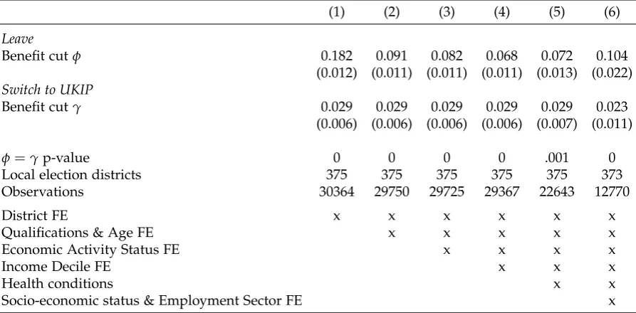
Pooled difference-in-difference The pooled difference-in-difference results are
presented in Table 2. The dependent variable in this table is a dummy
indicat-ing whether an individual expressed support for UKIP. Columns 2-4 provide es-timates for the three different welfare reforms affecting different subpopulations, 30Such shocks could be austerity-caused closures of libraries or parks. The fixed effects are also
while column 1 combines these into a single treatment indicator that is switched on from April 2013. The different Panels A - C employ different sets of fixed effects for the estimation. Panel A controls for district and region by survey-wave by time fixed effects. This empirical design comes closest to the estimations conducted in the previous sections by exploiting district-level variation. This empirical design comes closest to the estimations conducted in the previous sections by exploiting district-level variation. Across the different welfare reforms, the population likely exposed to a reform is significantly more likely to express support for UKIP af-ter these reforms became effective. The point estimates are economically sizable and precisely estimated, indicating that the treated population sees an increase in the propensity to support UKIP by between 2.6 - 5.1 percentage points. In rela-tive terms, the propensity to support UKIP increases by between 53 percent and 108 percent (relative to the mean of the dependent variable which stands at 4.7 percent). While the mean of the dependent variable appears low, suggesting that the effects are driven by a small subpopulation, it should be seen relative to lev-els of support for other political parties. The Liberal Democrats, the UK’s other main party, sees support in the USOC population averaging at just 8.2%; hence, the UKIP figures are not dramatically lower. In the next section, I explore a set of further outcomes to allay concerns about the validity of the outcome measure.
Panel B only exploits within-district variation, controlling for district by survey wave by time fixed effects. This effectively controls for any idiosyncratic and time-varying shocks affecting all residents in a specific districts. Such common shocks could, e.g. be capturing the indirect economic effects of austerity affecting the wider local economy or other local shocks. Throughout, the results remain very similar across the different measures.
Event studies I next turn to the event studies for the council tax benefit and the
bedroom tax.31 I begin by studying the abolishment of council tax benefit. The
results are presented visually in Figure 6. The left panel presents the average support for UKIP among those individuals who have consistently received council tax benefit at all times prior to its abolishment. The vertical line marks the date from which the council tax benefit was abolished. The propensity to support UKIP is consistently higher, on average, after the benefit was abolished which most likely affected this subpopulation. Panel B highlights that this subpopulation is indeed affected by the benefit cut; the share of individuals in the treated subpopulation stating that they are behind with their council tax payments rises sharply and in a very timely fashion. In Appendix Figure A5, I further highlight how, for this population, a marked and timely significant drop occurs in benefit income and gross income, while labor income remains unaffected.
Next, I turn to study the effects of the bedroom tax, which affected households on low incomes living in social housing. The results are presented in Figure7. The left panel presents the effects on support for UKIP among the group of individuals affected by the bedroom tax. While the pattern is noisier, there is a consistent in-crease in support for UKIP among this subpopulation. The central panel explores an economic margin directly relevant to those individuals who, likely, saw a cut to their housing benefit payment: they are significantly more likely to be in arrears with their rent, suggesting that the cut to housing benefit due to the spare bedroom increased rent arrears. Lastly, the right panel studies the number of bedrooms as an outcome variable, which is immediately relevant as the “bedroom tax” could be avoided if households moved to smaller accommodation. The pattern is quite consistent, suggesting that households started to move to smaller accommodation; while moving costs may not be negligible, this suggests that some households may have been able to avoid some of the direct economic grievances.
31The analysis of the disability living allowance reform is relegated to the Appendix FigureA6.
Together, these results provide further evidence in support of the underlying common trends assumption inherent to the previously presented difference-in-difference estimates. I next discuss a few additional robustness checks before studying broader measures of political dissatisfaction.
Accounting for other shocks While the event studies suggest that there are no
diverging pre-trends, some concerns may remain that the observed effects on sup-port for UKIP (and the auxiliary outcomes explored in the next section) could be masking other unobserved and concurrent shocks. A host of these concerns can be addressed by saturating the main estimation model with additional controls
as is done in Appendix TableA5, where column (1) replicates the corresponding
column (1) in Table 2 for reference. Columns (2) - (4) explore the implications of controlling for region-by-qualification-group or region-by-economic-activity status specific time effects. The former accounts for unobservable region and skill-group specific (labor market) shocks, while the latter accounts for the potential exposure to multiple concurrent policy shocks. (The economic activity status distinguishes between 11 different categories, such as being employed, retired, self-employed, a student, in a family care role, or being unemployed.)
Columns (5) and (6) further aim to account for a potentially (long-delayed) political response to the 2009 Recession. To address this issue, I construct an iden-tifier for each distinct economic activity status sequence that appears in the whole USOC panel. I then allow each such unique group that is identified by a dis-tinct economic activity status history to have a different set of time effects.32 This
adds to the estimation a further 18,000 unique estimable controls in the most de-manding specification and renders many observations perfectly collinear. Yet, the observation that exposure to either of the three reforms increases the propensity to support for UKIP remains broadly intact.
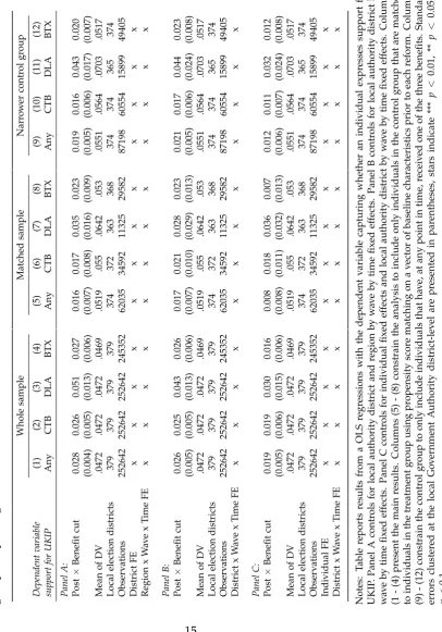
Refinement of the control group A second refinement of the analysis may
con-sist of restricting the control group. Naturally, this will have implications for the 32This would allow a separate non-linear time trend in political attitudes for certain cohorts. For
statistical power especially when estimation the more saturated models. I consider two such refinements. First, an ad hoc refinement that restricts the control group to those who at some point in time, have received the respective benefit or could have received it. An alternative approach to refine the control group uses propensity-score matching to construct matched pairs. For each reform, I construct matched pairs, with the matching based on: gender, age, dummy variables for the differ-ent economic-activity status, the housing-tenure status indicators, a set of features capturing the educational attainment across the five categories included in the UK census, along with the log value of pre-treatment monthly benefit income. This variable implies that matching will compare individuals with similar amounts of benefit income that differ only with respect to the specific benefit that is undergo-ing reform and is the subject of study. I impose a caliper of 0.01 to focus on good matches based on the baseline observables.The results from this exercise are added as Appendix Table A6, replicating the main results Table 2, but adding the esti-mates that are obtained restricting the control groups. The analysis highlights that the results are robust. Unsurprisingly, statistical power is lost when moving from the less demanding specifications to the most demanding specifications, which ab-sorb both individual-level and demanding district-level time effects, especially for the Disability Living Allowance reform and the bedroom tax. This loss of power is not a substantive concern as, for example, the specification on the matched panel in column (5) of Panel C, in excess of 18,000 parameters are estimated on a sample of just over 60,000 observations.
5.5 Broader outcome measures
Expressing political support for UKIP may only be one specific outcome mea-sure, but the political responses to austerity could be broader.
Support and like or dislike for other parties I first present results capturing
welfare reforms. There is also a weak reduction in those reporting that they would not vote for any party if there was an election tomorrow in Panel D. This would be indicative of a potential increase in turnout that has been suggested to be an important factor in driving populist support (seeGuiso et al., 2018). The analysis
presented in Appendix TableA7suggests that those who become UKIP supporters
are mostly original supporters of the Conservatives, Labour and a few other parties but only marginally from among those who initially reported that they support no party/would not vote. The welfare-reform induced gains for Labour are mostly drawn from this pool of people.
In Appendix Table A8, I present results drawing on measures of the intensity of like or dislikes of the three historic main political parties (the Conservatives, Labour and the Liberal Democrats) on a 10 point Likert scale. The results suggest
that, respondents affected by the combined any welfare reform measure are much
more likely to express a scores indicating strong dislike for the Conservative party.
Perception of politics more broadly In Table4, I present evidence for three addi-tional survey questions, asking whether individuals perceive that “Public officials do not care”, that they “Don’t have a say in what government does” and that “your vote is unlikely to make a difference”. Each of these auxiliary measures see a sig-nificant increase among individuals exposed to welfare reforms. Appendix Table
A9further highlights that the effects of exposure to welfare reforms on these aux-iliary outcomes go beyond what can be accounted for by an individuals’ political preferences. As we will see, these auxiliary outcomes are also correlates for Leave support, even after accounting for an individuals’ political party preference.33
The perception of having no political voice is something that was prominently leveraged in the EU referendum campaign, with voters being suggested that
vot-ing against EU membership is a vote against the status quo (Ford and Goodwin,
2017). The observed additional effects are consistent with the idea that austerity contributed to a feeling of disenfranchisement or disconnect from the established political parties and institutions, and encouraged voters to support more extreme policy positions or engage in protest voting (Myatt,2017). Unfortunately, despite 33Appendix TableA10further highlights that the effects on these auxiliary outcomes are broadly