Processing Modflow A Simulation System for Modeling Groundwater Flow and Pollution. Wen-Hsing Chiang and Wolfgang Kinzelbach

(1)

Processing Modflow

A Simulation System for Modeling Groundwater Flow and Pollution

Wen-Hsing Chiang and Wolfgang Kinzelbach

(2)

(3)

Preface

1. Introduction . . . 1

System Requirements . . . 4 Setting Up PMWIN . . . 4 Documentation . . . 4 Online Help . . . 5

2. Your First Groundwater Model with PMWIN . . . 7

2.1 Run a Steady-State Flow Simulation . . . 8

2.2 Simulation of Solute Transport . . . 32

2.2.1 Perform Transport Simulation with MT3D . . . 33

2.2.2 Perform Transport Simulation with MOC3D . . . 39

2.3 Automatic Calibration . . . 44

2.3.1 Perform Automatic Calibration with PEST . . . 46

2.3.2 Perform Automatic Calibration with UCODE . . . 49

2.4 Animation . . . 51

3. The Modeling Environment . . . 53

3.1 The Grid Editor . . . 55

3.2 The Data Editor . . . 59

3.2.1 The Cell-by-Cell Input Method . . . 61

3.2.2 The Zone Input Method . . . 62

3.2.3 Specification of Data for Transient Simulations . . . 63

3.3 The File Menu . . . 65

3.4 The Grid Menu . . . 69

3.5 The Parameters Menu . . . 74

3.6 The Models Menu . . . 80

3.6.1 MODFLOW . . . 80

3.6.2 MOC3D . . . 111

3.6.3 MT3D . . . 119

3.6.4 MT3DMS . . . 132

(4)

4.3 PMPATH Options Menu . . . 187

4.4 PMPATH Output Files . . . 195

5. Modeling Tools . . . 199

5.1 The Digitizer . . . 199

5.2 The Field Interpolator . . . 200

5.3 The Field Generator . . . 206

5.4 The Results Extractor . . . 208

5.5 The Water Balance Calculator . . . 210

5.6 The Graph Viewer . . . 210

6. Examples and Applications . . . 215

6.1 Tutorials . . . 215

6.1.1 Tutorial 1 - Unconfined Aquifer System with Recharge . . . 215

6.1.2 Tutorial 2 - Confined and unconfined Aquifer System with River . . . 232

6.2 Basic Flow Problems . . . 244

6.2.1 Determination of Catchment Areas . . . 244

6.2.2 Use of the General-Head Boundary Condition . . . 248

6.2.3 Simulation of a Two-layer Aquifer System in which the Top Layer Converts between Wet and Dry . . . 250

6.2.4 Simulation of a Water-table Mound resulting from Local Recharge . . . 253

6.2.5 Simulation of a Perched Water Table . . . 257

6.2.6 Simulation of an Aquifer System with Irregular Recharge and a Stream . 260 6.2.7 Simulation of a Flood in a River . . . 263

6.2.8 Simulation of Lakes . . . 266

(5)

6.4.1 Basic Model Calibration Skill with PEST/UCODE . . . 270

6.4.2 Estimation of Pumping Rates . . . 274

6.4.3 The Theis Solution - Transient Flow to a Well in a Confined Aquifer . . . 276

6.4.4 The Hantush and Jacob Solution - Transient Flow to a Well in a Leaky Confined Aquifer . . . 279

6.5 Geotechnical Problems . . . 282

6.5.1 Inflowof Water into an Excavation Pit . . . 282

6.5.2 Flow Net and Seepage under a Weir . . . 284

6.5.3 Seepage Surface through a Dam . . . 286

6.5.4 Cutoff Wall . . . 289

6.5.5 Compaction and Subsidence . . . 292

6.6 Solute Transport . . . 295

6.6.1 One-Dimensional Dispersive Transport . . . 295

6.6.2 Two-Dimensional Transport in a Uniform Flow Field . . . 297

6.6.3 Benchmark Problems and Application Examples from Liturature . . . 300

6.7 Miscellaneous Topics . . . 302

6.7.1 Using the Field Interpolator . . . 302

6.7.2 An Example of Stochastic Modeling . . . 306

7. Appendices . . . 309

Appendix 1: Limitation of PMWIN . . . 300

Appendix 2: Files and Formats . . . 310

Appendix 3: Input Data Files of the Supported Models . . . 315

Appendix 4: Internal Data Files of PMWIN . . . 318

Appendix 5: Using PMWIN with your MODFLOW . . . 324

Appendix 6: Running MODPATH with PMWIN . . . 326

(6)

(7)

Welcome to Processing Modflow: A Simulation System for Modeling Groundwater Flow and Pollution. Processing Modflow was originally developed for a remediation project of a disposal site in the coastal region of Northern Germany. At the beginning of the work, the code was designed as a pre- and postprocessor for the groundwater flow model MODFLOW. Several years ago, we began to prepare a Windows-version of Processing Modflow with the goal of bringing various codes together in a complete simulation system. The size of the program code grew, as we began to prepare the Windows-based advective transport model PMPATH and add options and features for supporting the solute transport models MT3D, MT3DMS and MOC3D and the inverse models PEST and UCODE.

As in the earlier versions of Processing Modflow, our goal is to provide an integrated groundwater modeling system with the hope that the very user-friendly implementation will lower the threshold which inhibits the widespread use of computer based groundwater models. To facilitate the use of Processing Modflow, more than 60 documented ready-to-run models are included in this software. Some of these models deal with theoretical background, some of them are of practical values.

The present text can be divided into three parts. The first two chapters introduce PMWIN with an example. Chapters 3 through 5 are a detalied description of the building blocks. Chapter 3 describes the use of Processing Modflow; chapter 4 describes the advection model PMPATH and chapter 5 introduces the modeling tools provided by Processing Modflow. The third part, Chapter 6, provides two tutorials and documents the examples.

Beside this text, we have gathered about 3,000 pages of documents related to the supported models. It is virtually not possible to provide all the documents in a printed form. So we decided to present these documents in an electronic format. The advantage of the electronic documents is considerable: with a single CD-ROM, you always have all necessary documents with you and we save resources by saving valuable papers and trees.

Many many people contributed to this modeling system. The authors wish to express heartfelt thanks to researchers and scientists, who have developed and coded the simulation programs MODFLOW, MOC3D, MT3D, MT3DMS, PEST and UCODE. Without their contributions, Processing Modflow would never have its present form. Many thanks are also due to authors of numerous add-on packages to MODFLOW.

We wish to thank many of our friends and colleagues for their contribution in developing, checking and validating the various parts of this software. We are very grateful to Steve Bengtson, John Doherty, Maciek Lubczynski, Wolfgang Schäfer, Udo Quek, Axel Voss and Jinhui Zhang who tested the software and provided many valuable comments and criticisms. For their encouragement and support, we thank Ian Callow, Lothar Moosmann, Renate Taugs, Gerrit van Tonder and Ray Volker. The authors also wish to thank Alpha Robinson, a scientist at the University of Paderborn, who checked Chapter 3 of this user’s guide. And thanks to our readers

(8)

(9)

1. Introduction

The applications of MODFLOW, a modular three-dimensional finite-difference groundwater model of the U. S. Geological Survey, to the description and prediction of the behavior of groundwater systems have increased significantly over the last few years. The “original” version of MODFLOW-88 (McDonald and Harbaugh, 1988) or MODFLOW-96 (Harbaugh and McDonald, 1996a, 1996b) can simulate the effects of wells, rivers, drains, head-dependent boundaries, recharge and evapotranspiration. Since the publication of MODFLOW various codes have been developed by numerous investigators. These codes are called packages, models or sometimes simply programs. Packages are integrated with MODFLOW, each package deals with a specific feature of the hydrologic system to be simulated, such as wells, recharge or river. Models or programs can be alone codes or can be integrated with MODFLOW. A stand-alone model or program communicates with MODFLOW through data files. The advective transport model PMPATH (Chiang and Kinzelbach, 1994, 1998), the solute transport model MT3D (Zheng, 1990), MT3DMS (Zheng and Wang, 1998) and the parameter estimation programs PEST (Doherty et al., 1994) and UCODE (Poeter and Hill, 1998) use this approach. The solute transport model MOC3D (Konikow et al., 1996) and the inverse model MODFLOWP (Hill, 1992) are integrated with MODFLOW. Both codes use MODFLOW as a function for calculating flow fields.

This text and the companion software Processing Modflow for Windows (PMWIN) offer a totally integrated simulation system for modeling groundwater flow and transport processes with MODFLOW-88, MODFLOW-96, PMPATH, MT3D, MT3DMS, MOC3D, PEST and UCODE. PMWIN comes with a professional graphical user-interface, the supported models and programs and several other useful modeling tools. The graphical user-interface allows you to create and simulate models with ease and fun. It can import DXF- and raster graphics and handle models with up to 1,000 stress periods, 80 layers and 250,000 cells in each model layer. The modeling tools include a Presentation tool, a Result Extractor, a Field Interpolator, a Field

Generator, a Water Budget Calculator and a Graph Viewer. The Result Extractor allows the

user to extract simulation results from any period to a spread sheet. You can then view the results or save them in ASCII or SURFER-compatible data files. Simulation results include hydraulic heads, drawdowns, cell-by-cell flow terms, compaction, subsidence, Darcy velocities, concentrations and mass terms. The Field Interpolator takes measurement data and interpolates the data to each model cell. The model grid can be irregularly spaced. The Water Budget

Calculator not only calculates the budget of user-specified zones but also the exchange of flows

between such zones. This facility is very useful in many practical cases. It allows the user to determine the flow through a particular boundary. The Field Generator generates fields with

(10)

1. Introduction

animation sequences using the simulation results (calculated heads, drawdowns or concentration). At present, PMWIN supports seven additional packages, which are integrated with the “original” MODFLOW. They are Time-Variant Specified-Head (CHD1), Direct Solution (DE45), Density (DEN1), Horizontal-Flow Barrier (HFB1), Interbed-Storage (IBS1), Reservoir (RES1) and Streamflow-Routing (STR1). The Time-Variant Specified-Head package (Leake et al., 1991) was developed to allow constant-head cells to take on different values for each time step. The Direct Solution package (Harbaugh, 1995) provides a direct solver using Gaussian elimination with an alternating diagonal equation numbering scheme. The Density package (Schaars and van Gerven, 1997) was designed to simulate the effect of density differences on the groundwater flow system. The Horizontal-Flow Barrier package (Hsieh and Freckleton, 1992) simulates thin, vertical low-permeability geologic features (such as cut-off walls) that impede the horizontal flow of ground water. The Interbed-Storage package (Leake and Prudic, 1991) simulates storage changes from both elastic and inelastic compaction in compressible fine-grained beds due to removal of groundwater. The Reservoir package (Fenske et al., 1996) simulates leakage between a reservoir and an underlying ground-water system as the reservoir area expands and contracts in response to changes in reservoir stage. The Streamflow-Routing package (Prudic, 1988) was designed to account for the amount of flow in streams and to simulate the interaction between surface streams and groundwater.

The particle tracking model PMPATH uses a semi-analytical particle tracking scheme (Pollock, 1988) to calculate the groundwater paths and travel times. PMPATH allows a user to perform particle tracking with just a few clicks of the mouse. Both forward and backward particle tracking schemes are allowed for steady-state and transient flow fields. PMPATH calculates and displays pathlines or flowlines and travel time marks simultaneously. It provides various on-screen graphical options including head contours, drawdown contours and velocity vectors.

The MT3D transport model uses a mixed Eulerian-Lagrangian approach to the solution of the three-dimensional advective-dispersive-reactive transport equation. MT3D is based on the assumption that changes in the concentration field will not affect the flow field significantly. This

(11)

1. Introduction allows the user to construct and calibrate a flow model independently. After a flow simulation is complete, MT3D simulates solute transport by using the calculated hydraulic heads and various flow terms saved by MODFLOW. MT3D can be used to simulate changes in concentration of single species miscible contaminants in groundwater considering advection, dispersion and some simple chemical reactions. The chemical reactions included in the model are limited to equilibrium-controlled linear or non-linear sorption and first-order irreversible decay or biodegradation.

MT3DMS is a further development of MT3D. The abbreviation MS denotes the Multi-Species structure for accommodating add-on reaction packages. MT3DMS includes three major classes of transport solution techniques, i.e., the standard finite difference method; the particle tracking based Eulerian-Lagrangian methods; and the higher-order finite-volume TVD method. In addition to the explicit formulation of MT3D, MT3DMS includes an implicit iterative solver based on generalized conjugate gradient (GCG) methods. If this solver is used, dispersion, sink/source, and reaction terms are solved implicitly without any stability constraints.

The MOC3D transport model computes changes in concentration of a single dissolved chemical constituent over time that are caused by advective transport, hydrodynamic dispersion (including both mechanical dispersion and diffusion), mixing or dilution from fluid sources, and mathematically simple chemical reactions, including decay and linear sorption represented by a retardation factor. MOC3D uses the method of characteristics to solve the transport equation on the basis of the hydraulic gradients computed with MODFLOW for a given time step. This implementation of the method of characteristics uses particle tracking to represent advective transport and explicit finite-difference methods to calculate the effects of other processes. For improved efficiency, the user can apply MOC3D to a subgrid of the primary MODFLOW grid that is used to solve the flow equation. However, the transport subgrid must have uniform grid spacing along rows and columns. Using MODFLOW as a built-in function, MOC3D can be modified to simulate density-driven flow and transport.

The purpose of PEST and UCODE is to assist in data interpretation and in model calibration. If there are field or laboratory measurements, PEST and UCODE can adjust model parameters and/or excitation data in order that the discrepancies between the pertinent model-generated numbers and the corresponding measurements are reduced to a minimum. Both codes do this by taking control of the model (MODFLOW) and running it as many times as is necessary in order to determine this optimal set of parameters and/or excitations.

(12)

1. Introduction

Software

A FORTRAN compiler is required if you intend to modify and compile the models MODFLOW-88, MODFLOW-96, MOC3D, MT3D or MT3DMS. For the reason of compability, the models must be compiled by a Lahey Fortran compiler. The source codes of the above-mentioned models are saved in the folder \Source\ of the CD-ROM.

Setting Up PMWIN

You install PMWIN on your computer using the self-installing program PM32010.EXE contained in the folder \programs\pm5\ of the CD-ROM. Please note: If you are using Windows NT 4.0, you must install the Service Pack 3 (or above) before installing PMWIN. Refer to the file readme.txt on the PM5 CD-ROM for more information.

Documentation

The folder \Document\ of the CD-ROM contains electronic documents in the Portable Document Format (PDF). You must first install the Acrobat®_{Reader before you can read or print the PDF} documents. You can find the installation file of the Acrobat®_{Reader in the folder}_\Reader\_. Execute the file \Reader\win95\ar302.exe from the CD directly and follow the screen to install the Reader.

Starting PMWIN

Once you have completed the installation procedure, you can start Processing Modflow by using the Start button on the task bar in Windows.

(13)

1. Introduction

Online Help

The online help system references nearly all aspects of PMWIN. You can access Help through the Help menu Contents command, by searching for specific topics with the Help Search tool, or by clicking the Help button to get context sensitive Help.

Help Search

The fastest way to find a particular topic in Help is to use the Search dialog box. To display the

Search dialog box, either choose Search from the Help menu or click the Search button on any Help topic screen.

<< To search Help

1. From the Help menu, choose Search. (You can also click the Search button from any Help topic window).

2. In the Search dialog box, type a word, or select one from the list by scrolling up or down. Press ENTER or choose Show Topics to display a list of topics related to the word you specified.

3. Select a topic and press ENTER or choose Go To to view the topic.

Context-Sensitive Help

Many parts of the PMWIN Help facility are context-sensitive. Context-sensitive means you can access help on any part of PMWIN directly by clicking the Help button or by pressing the F1 key.

Updates

Today the development of groundwater modeling techniques is progressing very rapidly, and a groundwater model must periodically be updated and expanded. For updates of PMWIN and our other software you may access the following web-pages on the Internet:

http://www.uovs.ac.za/igs/index.htm

(14)

(15)

Your First Groundwater Model with PMWIN

2. Your First Groundwater Model with PMWIN

It takes just a few minutes to build your first groundwater flow model with PMWIN. First, create a groundwater model by choosing New Model from the File menu. Next, determine the size of the model grid by choosing Mesh Size from the Grid menu. Then, specify the geometry of the model and set the model parameters, such as hydraulic conductivity, effective porosity etc.. Finally, perform the flow simulation by choosing MODFLOW<<Run... from the Models

menu.

After completing the flow simulation, you can use the modeling tools provided by PMWIN to view the results, to calculate water bugdets of particular zones, or graphically display the results, such as head contours. You can also use PMPATH to calculate and save pathlines or use the finite difference transport models MT3D or MOC3D to simulate transport processes.

This chapter provides an overview of the modeling process with PMWIN, describes the basic skills you need to use PMWIN, and takes you step by step through a sample problem. A complete reference for all menus and dialog boxes in PMWIN is contained in Chapter 3. The advective transport model PMPATH and the modeling tools are described in Chapter 4 and Chapter 5, respectively.

Overview of the Sample Problem

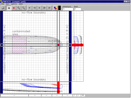
As shown in Fig. 2.1, an aquifer system with two stratigraphic units is bounded by no-flow boundaries on the North and South sides. The West and East sides are bounded by rivers, which are in full hydraulic contact with the aquifer and can be considered as fixed-head boundaries. The hydraulic heads on the west and east boundaries are 9 m and 8 m above reference level, respectively.

The aquifer system is unconfined and isotropic. The horizontal hydraulic conductivities of the first and second stratigraphic units are 0.0001 m/s and 0.0005 m/s, respectively. Vertical hydraulic conductivity of both units is assumed to be 10 percent of the horizontal hydraulic conductivity. The effective porosity is 25 percent. The elevation of the ground surface (top of the first stratigraphic unit) is 10m. The thickness of the first and the second units is 4 m and 6 m, respectively. A constant recharge rate of 8×10-9_{m/s is applied to the aquifer. A contaminated} area lies in the first unit next to the west boundary. The task is to isolate the contaminated area using a fully penetrating pumping well located next to the eastern boundary.

A numerical model has to be developed for this site to calculate the required pumping rate of the well. The pumping rate must be high enough, so that the contaminated area lies within the

(16)

2.1 Run a Steady-State Flow Simulation

Fig. 2.1 Configuration of the sample problem

concentration distribution after a simulation time of 3 years and display the breakthrough curves (concentration versus time) at two points [X, Y] = [290, 310], [390, 310] in both units.

2.1 Run a Steady-State Flow Simulation

Six main steps must be performed in a steady-state flow simulation: 1. Create a new model model

2. Assign model data

3. Perform the flow simulation 4. Check simulation results

5. Calculate subregional water budget 6. Produce output

(17)

Step 1: Create a New Model

The first step in running a flow simulation is to create a new model.

<< To create a new model

1. Choose New Model from the File menu. A New Model dialog box appears. Select a folder for saving the model data, such as C:\PM5DATA\SAMPLE, and type the file name SAMPLE for the sample model. A model must always have the file extension .PM5. All file names valid under Windows 95/98/NT with up to 120 characters can be used. It is a good idea to save every model in a separate folder, where the model and its output data will be kept. This will also allow you to run several models simultaneously (multitasking).

2. Click OK.

PMWIN takes a few seconds to create the new model. The name of the new model name is shown in the title bar.

Step 2: Assign Model Data

The second step in running a flow simulation is to generate the model grid (mesh), specify boundary conditions, and assign model parameters to the model grid.

PMWIN requires the use of consistent units throughout the modeling process. For example, if you are using length [L] units of meters and time [T] units of seconds, hydraulic conductivity will be expressed in units of [m/s], pumping rates will be in units of [m3_{/s] and} dispersivities will be in units of [m].

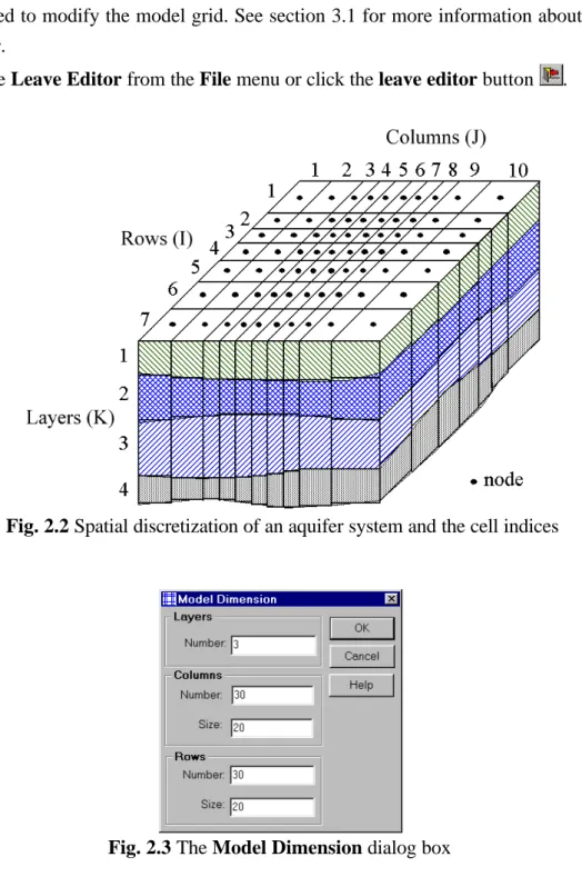
In MODFLOW, an aquifer system is replaced by a discretized domain consisting of an array of nodes and associated finite difference blocks (cells). Fig. 2.2 shows a spatial discretization of an aquifer system with a mesh of cells and nodes at which hydraulic heads are calculated. The nodal grid forms the framework of the numerical model. Hydrostratigraphic units can be represented by one or more model layers. The thicknesses of each model cell and the width of each column and row may be variable. The locations of cells are described in terms of columns, rows, and layers. PMWIN uses an index notation [J, I, K] for locating the cells. For example, the cell located in the 2nd column, 6th row, and the first layer is denoted by [2, 6, 1].

<< To generate the model grid

1. Choose Mesh Size from the Grid menu.

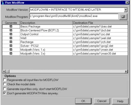
The Model Dimension dialog box appears (Fig. 2.3).

2. Enter 3 for the number of layers, 30 for the numbers of columns and rows, and 20 for the size of columns and rows.

(18)

Fig. 2.2 Spatial discretization of an aquifer system and the cell indices

(19)

Fig. 2.4 The generated model grid

Fig. 2.5 The Layer Options dialog box and the layer type drop-down list

The next step is to specify the type of layers.

<< To assign the type of layers

1. Choose Layer Type from the Grid menu. A Layer Options dialog box appears.

(20)

Note that a DXF-map is loaded by using the Maps Options. See Chapter 3 for details.

Now, you must specify basic boundary conditions of the flow model. The basic boundary contition array (IBOUND array) contains a code for each model cell which indicates whether (1) the hydraulic head is computed (active variable-head cell or active cell), (2) the hydraulic head is kept fixed at a given value (fixed-head cell or time-varying specified-head cell), or (3) no flow takes place within the cell (inactive cell). Use 1 for an active cell, -1 for a constant-head cell, and 0 for an inactive cell. For the sample problem, we need to assign -1 to the cells on the west and east boundaries and 1 to all other cells.

<< To assign the boundary condition to the flow model

1. Choose Boundary Condition << IBOUND (Modflow) from the Grid Menu.

The Data Editor of PMWIN appears with a plan view of the model grid (Fig. 2.6). The grid cursor is located at the cell [1, 1, 1], that is the upper-left cell of the first layer. The value of the current cell is shown at the bottom of the status bar. The default value of the IBOUND array is 1. The grid cursor can be moved horizontally by using the arrow keys or by clicking the mouse on the desired position. To move to an other layer, use PgUp or PgDn keys or click the edit field in the tool bar, type the new layer number, and then press enter.

2. Press the right mouse button. PMWIN shows a Cell Value dialog box. 3. Type -1 in the dialog box, then click OK.

The upper-left cell of the model has been specified to be a fixed-head cell. 4. Now turn on duplication by clicking the duplication button .

Duplication is on, if the relief of the duplication button is sunk. The current cell value will be duplicated to all cells passed by the grid cursor, if it is moved while duplication is on. You can turn off duplication by clicking the duplication button again.

5. Move the grid cursor from the upper-left cell [1, 1, 1] to the lower-left cell [1, 30, 1] of the model grid.

(21)

Fig. 2.6 Data Editor with a plan view of the model grid.

The value of -1 is duplicated to all cells on the west side of the model. 6. Move the grid cursor to the upper-right cell [30, 1, 1].

7. Move the grid cursor from the upper-right cell [30, 1, 1] to the lower-right cell [30, 30, 1]. The value of -1 is duplicated to all cells on the east side of the model.

8. Turn on layer copy by clicking the layer copy button .

Layer copy is on, if the relief of the layer copy button is sunk. The cell values of the current layer will be copied to other layers, if you move to the other model layer while layer copy is on. You can turn off layer copy by clicking the layer copy button again.

9. Move to the second layer and then to the third layer by pressing the PgDn key twice. The cell values of the first layer are copied to the second and third layers.

10. Choose Leave Editor from the File menu or click the leave editor button .

The next step is to specify the geometry of the model.

<< To specify the elevation of the top of model layers

1. Choose Top of Layers (TOP) from the Grid menu. PMWIN displays the model grid.

2. Choose Reset Matrix... from the Value menu (or press Ctrl+R). A Reset Matrix dialog box appears.

(22)

second and third layers to 6, 3 and 0, respectively.

3. Choose Leave Editor from the File menu or click the leave editor button .

We are going to specify the temporal and spatial parameters of the model. The spatial parameters for sample problem include the initial hydraulic head, horizontal and vertical hydraulic conductivities and effective porosity.

<< To specify the temporal parameters

1. Choose Time... from the Parameters menu.

A Time Parameters dialog box will come up. The temporal parameters include the time unit and the numbers of stress periods, time steps and transport steps. In MODFLOW, the simulation time is divided into stress periods - i.e., time intervals during which all external excitations or stresses are constant - which are, in turn, divided into time steps. In most transport models, each flow time step is further divided into smaller transport steps. The length of stress periods is not relevant to a steady state flow simulation. However, as we want to perform contaminant transport simulation with MT3D and MOC3D, the actual time length must be specified in the table.

2. Enter 9.46728E+07 (seconds) for Length of the first period. 3. Click OK to accept the other default values.

Now, you need to specify the initial hydraulic head for each model cell. The initial hydraulic head at a fixed-head boundary will be kept constant during the flow simulation. The other heads are starting values in a transient simulation or first guesses for the iterative solver in a steady-state simulation. Here we firstly set all values to 8 and then correct the values on the west side by overwriting them with a value of 9.

(23)

2.1 Run a Steady-State Flow Simulation 1. Choose Initial Hydraulic Heads from the Parameters menu.

PMWIN displays the model grid.

2. Choose Reset Matrix... from the Value menu (or press Ctrl+R) and enter 8 in the dialog box, then click OK.

3. Move the grid cursor to the upper-left model cell.

4. Press the right mouse button and enter 9 into the Cell Value dialog box, then click OK. 5. Now turn on duplication by clicking the duplication button .

Duplication is on, if the relief of the duplication button is sunk. The current cell value will be duplicated to all cells passed over by the grid cursor, if duplication is on.

6. Move the grid cursor from the upper-left cell to the lower-left cell of the model grid. The value of 9 is duplicated to all cells on the west side of the model.

Layer copy is on, if the relief of the layer copy button is sunk. The cell values of the current layer will be copied to another layer, if you move to the other model layer while layer copy is on.

8. Move to the second layer and the third layer by pressing PgDn twice. The cell values of the first layer are copied to the second and third layers. 9. Choose Leave Editor from the File menu or click the leave editor button .

<< To specify the horizontal hydraulic conductivity

1. Choose Horizontal Hydraulic Conductivity from the Parameters menu.

2. Choose Reset Matrix... from the Value menu (or press Ctrl+R), type 0.0001 in the dialog box, then click OK.

3. Move to the second layer by pressing PgDn.

5. Repeat steps 3 and 4 to set the value of the third layer to 0.0005.

<< To specify the vertical hydraulic conductivity

1. Choose Vertical Hydraulic Conductivity from the Parameters menu.

(24)

Q_k ' _Q

total @

T_k

ET (2.1)

<< To specify the recharge rate

1. Choose MODFLOW<< Recharge from the Models menu.

2. Choose Reset Matrix... from the Value menu (or press Ctrl+R), enter 8E-9 for Recharge

Flux [L/T] in the dialog box, then click OK.

The last step before performing the flow simulation is to specify the location of the pumping well and its pumping rate. In MODFLOW, an injection or pumping well is represented by a node (or a cell). The user specifies an injection or pumping rate for each node. It is implicitly assumed that the well penetrates the full thickness of the cell. MODFLOW can simulate the effects of pumping from a well that penetrates more than one aquifer or layer provided that the user supplies the pumping rate for each layer. The total pumping rate for the multilayer well is equal to the sum of the pumping rates from the individual layers. The pumping rate for each layer (Q_k) can be approximately calculated by dividing the total pumping rate (Q_total) in proportion to the layer transmissivities (McDonald and Harbaugh, 1988):

where T_k is the transmissivity of layer k and ET is the sum of the transmissivities of all layers penetrated by the multilayer well. Unfortunately, as the first layer is unconfined, we do not exactly know the saturated thickness and the transmissivity of this layer at the position of the well. Eq. 2.1 cannot be used unless we assume a saturated thickness for calculating the transmissivity. An other possibility to simulate a multi-layer well is to set a very large vertical hydraulic conductivity (or vertical leakance), e.g. 1 m/s, to all cells of the well. The total pumping rate is assigned to the lowest cell of the well. For the display purpose, a very small pumping rate (say, 1×10-10_m3_{/s) can be assigned to other cells of the well. In this way, the exact}

(25)

2.1 Run a Steady-State Flow Simulation extraction rate from each penetrated layer will be calculated by MODFLOW implicitly and the value can be obtained by using the Water Budget Calculator (see below).

As we do not know the required pumping rate for capturing the contaminated area shown in Fig. 2.1, we will try a total pumping rate of 0.0012 m3_/s.

<< To specify the pumping well and the pumping rate

1. Choose MODFLOW<<Well from the Models menu.

2. Move the grid cursor to the cell [25, 15, 1]

3. Press the right mouse button and type -1E-10, then click OK. Note that a negative value is used to indicate a pumping well.

5. Press the right mouse button and type -1E-10 then click OK. 6. Move to the third layer by pressing PgDn.

7. Press the right mouse button and type -0.0012 then click OK.

Step 3: Perform the Flow Simulation << To perform the flow simulation

1. Choose MODFLOW<<Run... from the Models menu.

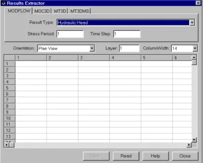
The Run Modflow dialog box appears (Fig. 2.7). 2. Click OK to start the flow computation.

Prior to running MODFLOW, PMWIN will use the user-specified data to generate input files for MODFLOW (and optionally MODPATH) as listed in the table of the Run

Modflow dialog box. An input file will be generated only if the generate flag is set to .

You can click on the button to toggle the generate flag between and . Generally, you do not need to change the flags, as PMWIN will care about the settings.

Step 4: Check Simulation Results

During a flow simulation, MODFLOW writes a detailed run record to the listing file path\OUTPUT.DAT, where path is the folder in which your model data are saved. If a flow simulation is successfully completed, MODFLOW saves the simulation results in various unformatted (binary) files as listed in Table 2.1. Prior to running MODFLOW, the user may control the output of these unformatted (binary) files by choosing Modflow<<Output Control

from the Models menu. The output file path\INTERBED.DAT will only be generated, if the Interbed Storage Package is activated (see Chapter 3 for details about the Interbed Storage Package).

(26)

Fig. 2.7 The Run Modflow dialog box

(27)

VOLUMETRIC BUDGET FOR ENTIRE MODEL AT END OF TIME STEP 1 IN STRESS PERIOD 1 CUMULATIVE VOLUMES L**3 RATES FOR THIS TIME STEP L**3/T ---

IN: IN:

CONSTANT HEAD = 209690.3590 CONSTANT HEAD = 2.2150E-03 WELLS = 0.0000 WELLS = 0.0000 RECHARGE = 254472.9380 RECHARGE = 2.6880E-03 TOTAL IN = 464163.3130 TOTAL IN = 4.9030E-03 OUT: OUT:

CONSTANT HEAD = 350533.6880 CONSTANT HEAD = 3.7027E-03 WELLS = 113604.0310 WELLS = 1.2000E-03 RECHARGE = 0.0000 RECHARGE = 0.0000 TOTAL OUT = 464137.7190 TOTAL OUT = 4.9027E-03 IN - OUT = 25.5938 IN - OUT = 2.7008E-07 PERCENT DISCREPANCY = 0.01 PERCENT DISCREPANCY = 0.01

Table 2.2 Volumetric budget for the entire model written by MODFLOW Table 2.1Output files from MODFLOW

File Contents

path\OUTPUT.DAT Detailed run record and simulation report

path\HEADS.DAT Hydraulic heads

path\DDOWN.DAT Drawdowns, the difference between the starting heads and the calculated hydraulic heads.

path\BUDGET.DAT Cell-by-Cell flow terms

path\INTERBED.DAT Subsidence of the entire aquifer and compaction and preconsolidation heads in individual layers.

path\MT3D.FLO Interface file to MT3D/MT3DMS. This file is created by the LKMT package provided by MT3D/MT3DMS (Zheng, 1990, 1998). - path is the folder in which the model data are saved.

Step 5: Calculate subregional water budget

There are situations in which it is useful to calculate water budgets for various subregions of the model. To facilitate such calculations, flow terms for individual cells are saved in the file path\BUDGET.DAT. These individual cell flows are referred to as cell-by-cell flow terms, and are of four types: (1) cell-by-cell stress flows, or flows into or from an individual cell due to one of the external stresses (excitations) represented in the model, e.g., pumping well or recharge; (2) cell-by-cell storage terms, which give the rate of accumulation or depletion of storage in an

(28)

Fig. 2.8 The Water Budget dialog box

not need to change the settings in the Time group. 2. Click Zones.

A zone is a subregion of a model for which a water budget will be calculated. A zone is indicated by a zone number ranging from 0 to 50. A zone number must be assigned to each model cell. The zone number 0 indicates that a cell is not associated with any zone. Follow steps 3 to 5 to assign zone numbers 1 to the first and 2 to the second layer.

3. Choose Reset Matrix... from the Value menu, type 1 in the dialog box, then click OK. 4. Press PgDn to move to the second layer.

5. Choose Reset Matrix... from the Value menu, type 2 in the dialog box, then click OK. 6. Choose Leave Editor from the File menu or click the leave editor button .

7. Click OK in the Water Budget dialog box.

PMWIN calculates and saves the flows in the file path\WATERBDG.DAT as shown in Table 2.3. The unit of the flows is [L3T-1]. Flows are calculated for each zone in each layer and each time step. Flows are considered IN, if they are entering a zone. Flows between subregions are given in a Flow Matrix. HORIZ. EXCHANGE gives the flow rate horizontally across the boundary of a zone. EXCHANGE (UPPER) gives the flow rate coming from (IN) or going to (OUT) to the upper adjacent layer. EXCHANGE (LOWER) gives the flow rate coming from

(29)

FLOWS ARE CONSIDERED "IN" IF THEY ARE ENTERING A SUBREGION THE UNIT OF THE FLOWS IS [L^3/T]

TIME STEP 1 OF STRESS PERIOD 1

ZONE= 1 LAYER= 1

FLOW TERM IN OUT IN-OUT STORAGE 0.0000000E+00 0.0000000E+00 0.0000000E+00 CONSTANT HEAD 1.8407618E-04 2.4361895E-04 -5.9542770E-05 HORIZ. EXCHANGE 0.0000000E+00 0.0000000E+00 0.0000000E+00 EXCHANGE (UPPER) 0.0000000E+00 0.0000000E+00 0.0000000E+00 EXCHANGE (LOWER) 0.0000000E+00 2.5872560E-03 -2.5872560E-03 WELLS 0.0000000E+00 1.0000000E-10 -1.0000000E-10 DRAINS 0.0000000E+00 0.0000000E+00 0.0000000E+00 RECHARGE 2.6880163E-03 0.0000000E+00 2.6880163E-03 . . . . . . . . SUM OF THE LAYER 2.8720924E-03 2.8308749E-03 4.1217543E-05 . . . . . . . .

FLOW TERM IN OUT IN-OUT STORAGE 0.0000000E+00 0.0000000E+00 0.0000000E+00 CONSTANT HEAD 1.0027100E-03 1.7383324E-03 -7.3562248E-04 HORIZ. EXCHANGE 0.0000000E+00 0.0000000E+00 0.0000000E+00 EXCHANGE (UPPER) 2.5872560E-03 0.0000000E+00 2.5872560E-03 EXCHANGE (LOWER) 0.0000000E+00 1.8930938E-03 -1.8930938E-03 WELLS 0.0000000E+00 1.0000000E-10 -1.0000000E-10 DRAINS 0.0000000E+00 0.0000000E+00 0.0000000E+00 RECHARGE 0.0000000E+00 0.0000000E+00 0.0000000E+00 . . . . . . . . SUM OF THE LAYER 3.5899659E-03 3.6314263E-03 -4.1460386E-05 . . . . . . . .

WATER BUDGET OF SELECTED ZONES:

IN OUT IN-OUT ZONE( 1): 2.8720924E-03 2.8308751E-03 4.1217310E-05 ZONE( 2): 3.5899659E-03 3.6314263E-03 -4.1460386E-05

---WATER BUDGET OF THE WHOLE MODEL DOMAIN:

FLOW TERM IN OUT IN-OUT STORAGE 0.0000000E+00 0.0000000E+00 0.0000000E+00 CONSTANT HEAD 2.2149608E-03 3.7026911E-03 -1.4877303E-03 WELLS 0.0000000E+00 1.2000003E-03 -1.2000003E-03 DRAINS 0.0000000E+00 0.0000000E+00 0.0000000E+00 RECHARGE 2.6880163E-03 0.0000000E+00 2.6880163E-03 . . . . . . . . SUM 4.9029770E-03 4.9026916E-03 2.8545037E-07 DISCREPANCY [%] 0.01

The value of the element (i,j) of the following flow matrix gives the flow rate from the i-th zone into the j-th zone. Where i is the column

index and j is the row index.

FLOW MATRIX:

1 2 ... 0 1 0.0000 0.0000 0 2 2.5873E-03 0.0000

Table 2.3 Output from the Water Budget Calculator

100 @ (IN & _OUT)

(IN % _{OUT) / 2} (2.2)

(IN) or going to (OUT) to the lower adjacent layer. For example, consider EXCHANGE (LOWER) of ZONE=1 and LAYER=1, the flow rate from the first layer to the second layer is 2.587256E-03 m3/s. The percent discrepancy in Table 2.3 is calculated by

(30)

FLOWS ARE CONSIDERED "IN" IF THEY ARE ENTERING A SUBREGION THE UNIT OF THE FLOWS IS [L^3/T]

TIME STEP 1 OF STRESS PERIOD 1

FLOW TERM IN OUT IN-OUT STORAGE 0.0000000E+00 0.0000000E+00 0.0000000E+00 CONSTANT HEAD 0.0000000E+00 0.0000000E+00 0.0000000E+00

HORIZ. EXCHANGE 7.7992809E-05 0.0000000E+00 7.7992809E-05

EXCHANGE (UPPER) 0.0000000E+00 0.0000000E+00 0.0000000E+00 EXCHANGE (LOWER) 0.0000000E+00 7.9696278E-05 -7.9696278E-05 WELLS 0.0000000E+00 1.0000000E-10 -1.0000000E-10 DRAINS 0.0000000E+00 0.0000000E+00 0.0000000E+00 RECHARGE 3.1999998E-06 0.0000000E+00 3.1999998E-06 . . . . . . . . SUM OF THE LAYER 8.1192811E-05 7.9696380E-05 1.4964317E-06 . . . . . . . .

EXCHANGE (UPPER) 7.9696278E-05 0.0000000E+00 7.9696278E-05 EXCHANGE (LOWER) 0.0000000E+00 6.4027577E-04 -6.4027577E-04 WELLS 0.0000000E+00 1.0000000E-10 -1.0000000E-10 . . . . . . . . SUM OF THE LAYER 6.4005010E-04 6.4027589E-04 -2.2578752E-07 ZONE= 3 LAYER= 3

EXCHANGE (UPPER) 6.4027577E-04 0.0000000E+00 6.4027577E-04 EXCHANGE (LOWER) 0.0000000E+00 0.0000000E+00 0.0000000E+00 WELLS 0.0000000E+00 1.2000001E-03 -1.2000001E-03 . . . . . . . . SUM OF THE LAYER 1.1979371E-03 1.2000001E-03 -2.0629959E-06

Table 2.4 Output from the Water Budget Calculator for the pumping well

Step 6: Produce Output

(31)

2.1 Run a Steady-State Flow Simulation results and creating graphical outputs. Pathlines and velocity vectors can be displayed by

PMPATH. Using the Results Extractor, simulation results of any layer and time step can be

read from the unformatted (binary) result files and saved in ASCII Matrix files. An ASCII Matrix file contains a value for each model cell in a layer. PMWIN can load ASCII matrix files into a model grid. The format of the ASCII Matrix file is described in Appendix 2. In the following, we will carry out the steps:

1. Use the Results Extractor to read and save the calculated hydraulic heads. 2. Generate a contour map based on the calculated hydraulic heads for the first layer. 3. Use PMPATH to compute pathlines as well as the capture zone of the pumping well.

<< To read and save the calculated hydraulic heads

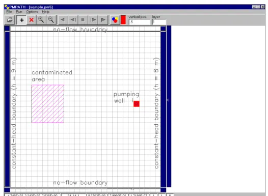
1. Choose Results Extractor... from the Tools menu

The Results Extractor dialog box appears (Fig. 2.9). The options in the Results Extractor dialog box are grouped under four tabs - MODFLOW, MOC3D, MT3D and MT3DMS. In the MODFLOW tab, you may choose a result type from the Result Type drop-down box. You may specify the layer, stress period and time step from which the result should be read. The spreadsheet displays a series of columns and rows. The intersection of a row and column is a cell. Each cell of the spreadsheet corresponds to a model cell in a layer. Refer to Chap. 5 for more detailed information about the Results Extractor. For the current sample problem, follow steps 2 to 6 to save the hydraulic heads of each layer in three ASCII Matrix files.

2. Choose Hydraulic Head from the Result Type drop-down box. 3. Type 1 in the Layer edit field.

For the current problem (steady-state flow simulation with only one stress period and one time step), the stress period and time step number should be 1.

4. Click Read.

Hydraulic heads in the first layer at time step 1 and stress period 1 will be read and put into the spreadsheet. You can scroll the spreadsheet by clicking on the scrolling bars next to the spreadsheet.

5. Click Save.

A Save Matrix As dialog box appears. By setting the Save as type option, the result can be optionally saved as an ASCII matrix or a SURFER data file. Specify the file name H1.DAT and select a folder in which H1.DAT should be saved. Click OK when ready. 6. Repeat steps 3, 4 and 5 to save the hydraulic heads of the second and third layer in the files

H2.DAT and H3.DAT, respectively. 7. Click Close to close the dialog box.

(32)

Note that PMWIN will clear the Visible check box when you leave the Editor.

results and use an additional Apply button in the Results Extractor dialog box to put the data into the Presentation matrix.

3. Click the Load... button.

The Load Matrix dialog box appears (Fig. 2.11).

4. Click and select the file H1.DAT, which was saved earlier by the Results Extractor. Click OK when ready. H1.DAT is loaded into the spreadsheet.

5. In the Browse Matrix dialog box, click OK. The Browse Matrix dialog box is closed.

6. Choose Environment from the Options menu (or Press Ctrl+E).

The Environment Options dialog box appears (Fig. 2.12). The options in the

Environment Options dialog box are grouped under three tabs. Appearance and Coordinate System allow the user to modify the appearance and position of the model grid.

Use Contours to generate contour maps.

7. Click the Contours tab, check Visible, then click the Restore Defaults button.

Clicking on the Restore Defaults button, PMWIN sets the number of contour lines to 11 and uses the maxmum and minimum values in the current layer as the minimum and maximum contour levels (Fig. 2.13). If Fill Contours is checked, the contours will be filled with the colors given in the Fill column of the table. Use Label Format button to specify an appropriate format.

8. In the Environment Options dialog box, Click OK.

PMWIN will redraw the model and display the contours (Fig. 2.14).

9. To save or print the graphics, choose Save Plot As... or Print Plot... from the File menu. 10. Press PgDn to move to the second layer. Repeat steps 2 to 9 to load the file H2.DAT,

display and save the plot.

(33)

Fig. 2.9 The Results Extractor dialog box.

Fig. 2.10 The Browse Matrix dialog box

to save changes to Presentation.

Using the procedure described above, you can generate contour maps based of your input data, any kind of simulation results or any data saved as an ASCII Matrix file. For example, you can create a contour map of the starting heads or you can use the Result Extractor to read the concentration distribution and display the contours. You can also generate contour maps of the fields created by the Field Interpolator or Field Generator. See chapter 5 for details about the Field Interpolator and Field Generator.

(34)

Fig. 2.13 The Contours options of the Environment Options dialog box Fig. 2.12 The Environment Options dialog box

(35)

Fig. 2.14 A contour map of the hydraulic heads in the first layer

Note that if you subsequently modify and calculate a model within PMWIN, you must load the modified model into PMPATH again to ensure that the modifications can be recognized by PMPATH. To load a model, click and select a model file with the extension .PM5 from the

Open Model dialog box.

<< To delineate the capture zone of the pumping well

1. Choose PMPATH (Pathlines and Contours) from the Models menu.

PMWIN calls the advective transport model PMPATH and the current model will be loaded into PMPATH automatically. PMPATH uses a "grid cursor" to define the column and row for which the cross-sectional plots should be displayed. You can move the grid cursor by holding down the Ctrl-key and click the left mouse button on the desired position.

2. To calculate the capture zone of the pumping well: a. Click the Set Particle button

b. Move the mouse cursor to the model area. The mouse cursor turns into crosshairs. c. Place the crosshairs at the upper-left corner of the pumping well, as shown in Fig. 2.15. d. Hold down the left moust button and drag the crosshairs until the window covers the

pumping well.

(36)

2.1 Run a Steady-State Flow Simulation zone of the pumping well (Fig. 2.17).

To see the projection of the pathlines on the cross-section windows in greater details, open an

Environment Options dialog box by choosing Environment... from the Options menu and set

a larger exaggeration value for the vertical scale in the Cross Sections tab. Fig. 2.18 shows the same pathlines by setting the vertical exaggeration value to 10. Note that some pathlines end up at the groundwater surface, where recharge occurs. This is one of the major differences between a three-dimensional and a two-dimensional model. In two-dimensional areal simulation models, such as ASM for Windows (Chiang et al., 1998), FINEM (Kinzelbach et al, 1990) or MOC (Konikow and Bredehoeft, 1978), a vertical velocity term does not exist (or always equals to zero). This leads to the result that pathlines can never be tracked back to the ground surface where the groundwater recharge from the precipitation occurs.

PMPATH can create time-related capture zones of pumping wells. The 100-days-capture zone shown in Fig. 2.19 is created by using the settings in the Particle Tracking (Time)

Properties dialog box (Fig. 2.20) and clicking . To open this dialog box, choose Particle

Tracking (Time)... from the Options menu. Note that because of lower hydraulic conductivity

(and thus lower flow velocity) the capture zone in the first layer is smaller than those in the other layers.

(37)

Fig. 2.15 The sample model loaded in PMPATH

(38)

Fig. 2.17 The capture zone of the pumping well (with vertical exaggeration=1)

(39)

Fig. 2.19 100-days-capture zone calculated by PMPATH

(40)

The Modeling Environment - 3.1 The Grid Editor

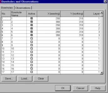
Fig. 2.21 The Boreholes and Observations dialog box

The hydrodynamic dispersion can be expressed in terms of the dispersivity [L] and the coefficient of molecular diffusion [L2_T-1_{] for the solute in the porous medium. The types of} reactions incorporated into MOC3D are restricted to those that can be represented by a first-order rate reaction, such as radioactive decay, or by a retardation factor, such as instaneous, reversible, sorption-desorption reactions goverened by a linear isotherm and constant distribution coefficient (K_d). In addition to the linear isotherm, MT3D supports non-linear isotherms, i.e., Freundlich and Langmuir isotherms.

Prior to running MT3D or MOC3D, you need to define the observation boreholes, for which the breakthrough curvers will be calculated.

<< To define observation boreholes

1. Choose Boreholes and Observations from the Paramters menu.

A Boreholes and Observations dialog box appears. Enter the coordinates of the observation boreholes into the dialog box as shown in Fig. 2.21.

(41)

2.2.1 Perform Transport Simulation with MT3D

2.2.1 Perform Transport Simulation with MT3D

MT3D requires a boundary condition code for each model cell which indicates whether (1) solute concentration varies with time (active concentration cell), (2) the concentration is kept fixed at a constant value (constant-concentration cell), or (3) the cell is an inactive concentration cell. Use 1 for an active concentration cell, -1 for a constant-concentration cell, and 0 for an inactive concentration cell. Active, variable-head cells can be treated as inactive concentration cells to minimize the area needed for transport simulation, as long as the solute concentration is insignificant near those cells.

Similar to the flow model, you must specify the initial concentration for each model cell. The initial concentration at a constant-concentration cell will be kept constant during a transport simulation. The other concentration are starting values in a transport simulation.

<< To assign the boundary condition to MT3D

1. Choose Boundary Conditions << ICBUND (MT3D/MT3DMS) from the Grid menu.

For the current example, we accept the default value 1 for all cells.

<< To set the initial concentration

1. Choose MT3D << Initial Concentration from the Models menu.

For the current example, we accept the default value 0 for all cells.

<< To assign the input rate of contaminants

1. Choose MT3D << Sink/Source Concentration << Recharge from the Models menu.

2. Assign 12500 [µg/m3_{] to the cells within the contaminated area.}

This value is the concentration associated with the recharge flux. Since the recharge rate is 8 × 10-9 [m3/m2/s] and the dissolution rate is 1 × 10-4 [µg/s/m2], the concentration associated with the recharge flux is 1 × 10-4_{/ 8 × 10}-9_{= 12500 [µg/m}3_]

<< To assign the transport parameters to the Advection Package

1. Choose MT3D << Advection... from the Models menu.

An Advection Package (MTADV1) dialog box appears. Enter the values as shown in Fig. 2.22 into the dialog box, select Method of Characteristics (MOC) for the solution scheme and First-order Euler for the particle tracking algorithm.

(42)

Fig. 2.22 The Advection Package (MTADV1) dialog box

<< To assign the dispersion parameters

1. Choose MT3D << Dispersion... from the Models menu.

A Dispersion Package (MT3D) dialog box appears. Enter the ratios of the transverse dispersivity to longitudinal dispersivity as shown in Fig. 2.23.

2. Click OK.

PMWIN displays the model grid. At this point you need to specify the longitudinal dispersivity to each cell of the grid.

3. Choose Reset Matrix... from the Value menu (or press Ctrl+R), type 10 in the dialog box then click OK.

5. Move to the second layer and the third layer by pressing PgDn twice. The cell values of the first layer are copied to the second and third layers. 6. Choose Leave Editor from the File menu or click the leave editor button .

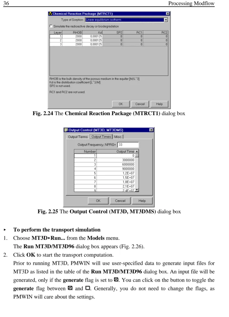
<< To assign the chemical reaction parameters

1. Choose MT3D << Chemical Reaction << Layer by Layer from the Models menu.

A Chemical Reaction Package (MTRCT1) dialog box appears. Clear the check box

(43)

R ' ₁ % Db

n @ Kd (2.3)

Fig. 2.23 The Advection Package (MTADV1) dialog box

isotherm for the type of sorption. For the linear isotherm, the retardation factor R for each

cell is calculated at the beginning of the simulation by

Where n [-] is the effective porosity with respect to the flow through the porous medium, Db

[ML-3_{] is the bulk density of the porous medium and}_K

d [L3M-1] is the distribution coefficient

of the solute in the porous medium. As the effective porosity is equal to 0.25, setting

Db = 2000 and Kd = 0.000125 yields R = 2.

2. Click OK to close the Chemical Reaction Package (MTRCT1) dialog box (Fig. 2.24).

The last step before running the transport model is to specify the output times, at which the calculated concentration should be saved.

<< To specify the output times

1. Choose MT3D << Output Control... from the Models menu.

An Output Control (MT3D, MT3DMS) dialog box appears. The options in this dialog box are grouped under three tabs - Output Terms, Output Times and Misc.

2. Click the Output Times tab, then click the header Output Time of the (empty) table. An Output Times dialog box appears. Enter 3000000 to Interval in this dialog box then click OK to accept the other defalut values.

(44)

Fig. 2.24 The Chemical Reaction Package (MTRCT1) dialog box

Fig. 2.25 The Output Control (MT3D, MT3DMS) dialog box

<< To perform the transport simulation

1. Choose MT3D<<Run... from the Models menu.

The Run MT3D/MT3D96 dialog box appears (Fig. 2.26). 2. Click OK to start the transport computation.

Prior to running MT3D, PMWIN will use user-specified data to generate input files for MT3D as listed in the table of the Run MT3D/MT3D96 dialog box. An input file will be generated, only if the generate flag is set to . You can click on the button to toggle the

generate flag between and . Generally, you do not need to change the flags, as

(45)

Fig. 2.26 The Run MT3D/MT3D96 dialog box << Check simulation results and produce output

During a transport simulation, MT3D writes a detailed run record to the file path\OUTPUT.MT3, where path is the folder in which your model data are saved. MT3D saves the simulation results in various files, which can be controlled by choosing MT3D << Output Control... from the Models menu.

To check the quality of the simulation results, a mass budget is calculated at the end of each transport step and accumulated to provide summarized information on the total mass into or out of the groundwater flow system. The discrepancy between the total mass in and out servers as an indicator of the accuracy of the simulation results. It is highly recommended to check the record file or at least take a glance at it.

Using Presentation you can generate contour maps of the calculated concentration. Fig. 2.27 shows the calculated concentration in the third layer at the end of the simulation (simulation time=9.467E+07 seconds).

To generate the breakthrough curves, choose Graphs << Concentration Time << MT3D

from the Tools menu. Click on the Plot flags of the Boreholes table until they are set to (Fig. 2.28).

(46)

Fig. 2.27 Simulated concentration at 3 years in the third layer

(47)

2.2.2 Perform Transport Simulation with MOC3D

Fig. 2.29 The Subgrid for Transport (MOC3D) dialog box. 2.2.2 Perform Transport Simulation with MOC3D

In MOC3D, transport may be simulated within a subgrid, which is a “window” within the primary model grid used to simulate flow. Within the subgrid, the row and column spacing must be uniform, but the thickness can vary from cell to cell and layer to layer. However, the range in thickness values (or product of thickness and effective porosity) should be as small as possible. The initial concentration must be specified throughout the subgrid within which solute transport occurs. MOC3D assumes that the concentration outside of the subgrid is the same within each layer, so only one value is specified for each layer within and adjacent to the subgrid. The use of constant-concentration boundary condition has not been implemented in MOC3D.

<< To set the initial concentration

1. Choose MOC3D << Initial Concentration from the Models menu.

For the current example, we accept the default value 0 for all cells. Note that PMWIN automatically uses the same initial concentration values for both MOC3D and MT3D. 2. Choose Leave Editor from the File menu or click the leave editor button .

<< To define the transport subgrid and the concentration outside of the subgrid

1. Choose MOC3D << Subgrid... from the Models menu.

The Subgrid for Transport (MOC3D) dialog box appears (Fig. 2.29). The options in the dialog box are grouped under two tabs - Subgrid and C’ Outside of Subgrid. The default size of the subgrid is the same as the model grid used to simulate flow. The default initial concentration outside of the subgrid is zero. We will accept the defaults.

(48)

Fig. 2.30 The Parameters for Advective Transport dialog box.

1. Choose MOC3D << Advection... from the Models menu.

A Parameters for Advection Transport (MOC3D) dialog box appears. Enter the values as shown in Fig. 2.30 into the dialog box, select Bilinear (X, Y directions) for the interpolation scheme for particle velocity. As noted by Konikow et al. (1996), if transmissivity within a layer is homogeneous or smoothly varying, bilinear interpolation of velocity yields more realistic pathlines for a given discretization than does linear interpolation.

2. Click OK to close the dialog box.

<< To assign the parameters for dispersion and chemical reaction

1. Choose MOC3D << Dispersion & Chemical Reaction... from the Models menu.

A Dispersion / Chemical Reaction (MOC3D) dialog box appears. Check Simulate

Dispersion and enter the values as shown in Fig. 2.31. Note that the parameters for

dispersion and chemical reaction are the same for each layer. 2. Click OK to close the dialog box.

(49)

Fig. 2.31 The Dispersion / Chemical Reaction (MOC3D) dialog box. << To set Strong/Weak Flag

1. Choose MOC3D << Strong/Weak Flag from the Models menu.

2. Move the grid cursor to the cell [25, 15, 1].

3. Press the right mouse button and type 1, then click OK. Note that a strong sink or source is indicated by the value of 1 in the matrix. When a fluid source is “strong”, new particles are added to replace old particles as they are advected out of that cell. Where a fluid sink is “strong”, particles are removed after they enter that cell.

4. Repeat steps 2 and 3 to assign the value 1 to the cells [25, 15, 2] and [25, 15, 3]. 5. Choose Leave Editor from the File menu or click the leave editor button .

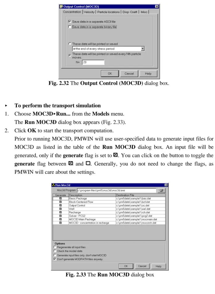
<< To specify the output terms and times

1. Choose MOC3D << Output Control... from the Models menu.

An Output Control (MOC3D) dialog box appears. The options in the dialog box are grouped under five tabs - Concentration, Velocity, Particle Locations, Disp. Coeff. and

Misc.

2. In the Concentration tab, select the option These data will be printed or saved every

Nth particle moves and enter N = 20.

3. Click OK to accept all other default values and close the Output Control (MOC3D) dialog box (Fig. 2.32).

(50)

Fig. 2.32 The Output Control (MOC3D) dialog box.

Fig. 2.33 The Run MOC3D dialog box << To perform the transport simulation

1. Choose MOC3D<<Run... from the Models menu.

The Run MOC3D dialog box appears (Fig. 2.33). 2. Click OK to start the transport computation.

Prior to running MOC3D, PMWIN will use user-specified data to generate input files for MOC3D as listed in the table of the Run MOC3D dialog box. An input file will be generated, only if the generate flag is set to . You can click on the button to toggle the

generate flag between and . Generally, you do not need to change the flags, as

(51)

Fig. 2.34 Simulated concentration at 3 years in the third layer << Check simulation results and produce output

During a transport simulation, MOC3D writes a detailed run record to the file path\MOC3D.LST, where path is the folder in which your model data are saved. MOC3D saves the simulation results in various files, which can be controlled by choosing MOC3D << Output Control... from the Models menu.

To check the quality of the simulation results, mass balance calculations are performed and saved in the run record file. The mass in storage at any time is calculated from the concentrations at the nodes of the transport subgrid to provide summarized information on the total mass into or out of the groundwater flow system. The mass balance error will typically exhibit an oscillatory behavior over time, because of the finite-difference approximation and the nature of the method of characteristics. As discussed in Konikow et al. (1996), as long as the oscillations remain within a steady range, not exceeding about ±10 percent as a guide, then the error probably does not represent a bias and is not a serious problem. Rather, the ocillations only reflect the fact that the mass balance calculation is itself just an approximation.

Using Presentation you can generate contour maps of the calculated concentration. Fig. 2.34 shows the calculated concentration at 3 years in the third layer (simulation time=9.467E+07 seconds).

To generate the breakthrough curves, choose Graphs << Concentration Time << MOC3D

from the Tools menu. Click on the Plot flags of the Boreholes table until they are set as in Fig. 2.35.

(52)

2.3 Automatic Calibration

Fig. 2.35 Concentration-time curves at the observation boreholes

2.3 Automatic Calibration

Calibration of a flow model is accomplished by finding a set of parameters, hydrologic stresses or boundary conditions so that the simulated heads or drawdowns match the measurement values to a reasonable degree. The calibration process is one of the most difficult and critical steps in the model application. Hill (1998) gives methods and guidelines for model calibration using inverse modeling.

To demonstrate the use of the inverse models PEST and UCODE within PMWIN, we assume that the hydraulic conductivity in the third layer is homogeneous but its value is unknown. We want to find out this value through a model calibration by using the measured hydraulic heads at the observation boreholes listed below.

Borehole X-coordinate Y-coordinate Layer Hydraulic Head

1 130 200 3 8.85

2 200 400 3 8.74

3 480 250 3 8.18