systems
.
White Rose Research Online URL for this paper:
http://eprints.whiterose.ac.uk/798/
Article:
Liu, G.P.P., Kadirkamanathan, V. and Billings, S.A. (1999) Variable neural networks for
adaptive control of nonlinear systems. IEEE Transactions on Systems Man and
Cybernetics Part C: Applications and Reviews, 29 (1). pp. 34-43. ISSN 1094-6977
https://doi.org/10.1109/5326.740668
[email protected] https://eprints.whiterose.ac.uk/ Reuse
Unless indicated otherwise, fulltext items are protected by copyright with all rights reserved. The copyright exception in section 29 of the Copyright, Designs and Patents Act 1988 allows the making of a single copy solely for the purpose of non-commercial research or private study within the limits of fair dealing. The publisher or other rights-holder may allow further reproduction and re-use of this version - refer to the White Rose Research Online record for this item. Where records identify the publisher as the copyright holder, users can verify any specific terms of use on the publisher’s website.
Takedown
If you consider content in White Rose Research Online to be in breach of UK law, please notify us by
Variable Neural Networks for Adaptive
Control of Nonlinear Systems
Guoping P. Liu,
Member, IEEE, Visakan Kadirkamanathan,Member, IEEE, and Stephen A. BillingsAbstract— This paper is concerned with the adaptive control
of continuous-time nonlinear dynamical systems using neural networks. A novel neural network architecture, referred to as a variable neural network, is proposed and shown to be useful in approximating the unknown nonlinearities of dynamical systems. In the variable neural networks, the number of basis functions can be either increased or decreased with time according to specified design strategies so that the network will not overfit or underfit the data set. Based on the Gaussian radial basis function (GRBF) variable neural network, an adaptive control scheme is presented. The location of the centers and the determination of the widths of the GRBF’s in the variable neural network are analyzed to make a compromise between orthogonality and smoothness. The weight adaptive laws developed using the Lya-punov synthesis approach guarantee the stability of the overall control scheme, even in the presence of modeling error. The tracking errors converge to the required accuracy through the adaptive control algorithm derived by combining the variable neural network and Lyapunov synthesis techniques. The oper-ation of an adaptive control scheme using the variable neural network is demonstrated using two simulated examples.
Index Terms— Adaptive control, neural networks, nonlinear
systems, radial basis functions.
I. INTRODUCTION
N
EURAL networks are capable of learning and recon-structing complex nonlinear mappings and have been widely studied by control researchers in the identification analysis and design of control systems. A large number of control structures have been proposed, including supervised control [55], direct inverse control [34], model reference con-trol [39], internal model concon-trol [13], predictive concon-trol [14], [56], [29], gain scheduling [12], optimal decision control [10], adaptive linear control [7], reinforcement learning control [1], [3], variable structure control [30], indirect adaptive control [39], and direct adaptive control [19], [45], [50], [51]. The principal types of neural networks used for control problems are the multilayer perceptron (MLP) neural networks with sigmoidal units [34], [39], [48] and the radial basis function (RBF) neural networks [41], [43], [47].Manuscript received September 4, 1995; revised September 9, 1996 and November 8, 1997. This work was supported by the Engineering and Physical Sciences Research Council (EPSRC) of the United Kingdom under Contract GR/J46661.
G. P. Liu is with the ALSTOM Energy Technology Centre, LE8 6LH Leicester, U.K. (e-mail: [email protected]).
V. Kadirkamanathan and S. A. Billings are with the Department of Automatic Control and Systems Engineering, University of Sheffield, S1 3JD Sheffield, U.K.
Publisher Item Identifier S 1094-6977(99)00100-5.
Most of the neural network-based control schemes view the problem as deriving adaptation laws using a fixed structure neural network. However, choosing this structure, such as the number of basis functions (hidden units in a single hidden layer) in the neural network, must be done a priori. This can often lead to either an overdetermined or an underdetermined network structure. In the discrete-time formulation, some approaches have been developed to determine the number of hidden units (or basis functions) using decision theory [4] and model comparison methods, such as minimum description
length [54] and Bayesian methods [33]. The problem with
these methods is that they require all observations to be available and hence are not suitable for online control tasks, especially adaptive control. In addition, the fixed structure neural networks often need a large number of basis functions even for simple problems.
Another type of neural network structure developed for learning systems is to begin with a larger network and then to prune this [32], [36], or to begin with a smaller network and then to expand this [9], [42] until the optimal network complexity is found. Among these dynamic structure models, the resource allocating network (RAN) developed by Platt [42] is an online or sequential identification algorithm. The RAN is essentially a growing Gaussian radial basis function (GRBF) network whose growth criteria and parameter adaptation laws have been studied and extended further [20], [21], [31] and applied to time-series analysis [24] and pattern classification [23]. The RAN and its extensions addressed the identification of only autoregressive systems with no external inputs and hence stability was not an issue. Recently, the growing GRBF neural network has been applied to sequential identification and adaptive control of dynamical continuous nonlinear sys-tems with external inputs [8], [22], [27], [28]. Though the growing neural network is much better than the fixed neural network in reducing the number of basis functions, it is still possible that this network will induce an overfitting problem. There are two main reasons for this. It is difficult to know how many basis functions are really needed for the problem, and secondly, the nonlinearity of a nonlinear function to be modeled is different when its variables change their value ranges. Normally, the number of basis functions in the growing neural network may increase to the one that the system needs to meet the requirement for dealing with the most complicated nonlinearity (the worst case) of the nonlinear function. Thus, it may lead to a network that has the same size as the fixed neural networks.
To overcome the above limitations, a new network structure, referred to as the variable neural network, is proposed in this paper. The basic principle of the variable neural network is that the number of basis functions in the network can be either increased or decreased over time according to a design strategy in an attempt to avoid overfitting or underfitting. In order to model unknown nonlinearities, the variable neural network starts with a small number of initial hidden units and then adds or removes units located in a variable grid. This grid consists of a number of subgrids composed of different sized hypercubes that depend on the novelty of the observation. Since the novelty of the observation is tested, it is ideally suited for online control problems. The objective behind the development is to gradually approach the appropriate network complexity that is sufficient to provide an approximation to the system nonlinearities and consistent with the observations being received. By allocating GRBF units on a variable grid, only the relevant state-space traversed by the dynamical system is spanned, resulting in considerable savings on the size of the network.
The parameters of the variable neural network are adjusted by adaptation laws developed using the Lyapunov synthesis approach. Combining the variable neural network and Lya-punov synthesis techniques, the adaptive control algorithm developed for continuous dynamical nonlinear systems guar-antees the stability of the whole control scheme and the convergence of the tracking errors between the reference inputs and the outputs.
The remainder of the paper is organized as follows. In Section II, the modeling of nonlinear dynamical systems by the GRBF network is discussed and a one-to-one mapping of the state-space to form a compact network input space is intro-duced. In Section III, a variable neural network is developed, based on a proposed variable grid. The selection of the GRBF’s for the variable neural network is discussed. The adaptive control scheme using the variable neural networks and the Lyapunov synthesis techniques is developed in Section IV. The stability of the overall control scheme and the convergence of the tracking errors are also analyzed. The operation of the adaptive control scheme is demonstrated by two simulated examples in Section V.
II. NONLINEAR SYSTEMMODELING
Consider a class of continuous nonlinear dynamical systems that can be expressed in the canonical form [18], [40], [53]
(1)
where is the output, is the control input, is the th derivative of the output with respect to time, and and are unknown nonlinear functions. The above system represents a class of continuous-time nonlinear systems, called affine systems. The above equation can also be transformed to the state-space form
(2)
(3)
where
(4)
, is an identity matrix,
and is the state vector.
Due to some desirable features, such as local adjustment of weights and mathematical tractability, RBF networks have recently attracted considerable attention (see, for example, [2], [5], [6], and [26]). Their importance has also greatly benefited from the work of Moody and Darken [35] and Poggio and Girosi [44], who explored the relationship between regular-ization theory and RBF networks. The good approximation properties of the RBF’s in interpolation have been well studied by Powell and his group [47]. With the use of Gaussian activation functions, each basis function in the RBF network responds only to inputs in the neighborhood determined by the center and width of the function. It is also known that, if the variables of a nonlinear function are in compact sets, the continuous function can be approximated arbitrarily well by GRBF networks [43]. Here, the GRBF networks are used to model the nonlinearity of the system.
If is not in a certain range, we introduce the following one-to-one (1-1) mapping [27]:
for (5)
where are positive constants, which can be chosen by the designer (e.g., are one). Thus, it is clear from (5)
that for . The above
one-to-one mapping shows that, in the -dimensional space, the entire area can be transferred into an -dimensional hypercube denoted by the compact set . Clearly, if is already in the desired area, we only need to set .
Thus, the nonlinear part of the system can be described by the following GRBF network:
(6)
where
(7)
for
(8)
and
are the optimal weight vectors, is the variable vector, is the th center, is the th width, is the modeling error, and is the number of the basis functions. It is known from approximation theory that the modeling error can be reduced arbitrarily by increasing the number , i.e., the number of the linear independent basis functions in the network model. Thus, it is reasonable to assume that the modeling error is bounded by a constant , which represents the accuracy of the model, and this is defined as
Although can be reduced arbitrarily by increasing the number of the independent basis functions, generally, when the number is greater than a small value, the modeling error is improved very little by increasing the number further. It also results in a large-sized network even for a simple problem. In practice, this is not realistic. In most cases, the required modeling error can be given by considering the design requirements and specifications of the system. Thus, the problem now is to find a suitable-sized network to achieve the required modeling error. In other words, it is how to determine the number, centers, widths, and weights of the GRBF’s in the network.
III. VARIABLENEURAL NETWORKS
Two main neural network structures that are widely used in online identification and control are the fixed neural network and the growing neural network. The fixed neural network usually needs a large number of basis functions in most cases even for a simple problem. Though the growing network is much better than the fixed network in reducing the number of the basis functions for a number of problems, it is still possible that this network will lead to an overfitting problem for some cases, and this is explained in Section I. To overcome the above limitations of the fixed and growing neural networks, a new network structure, called the variable neural network, is proposed in this section.
A. Variable Grid
In GRBF networks, the very important parameter is the location of the centers of the GRBF’s over the compact set , which is the approximation region. Usually, an -dimension grid is used to locate all centers in the gridnodes [51]. Thus, the distance between the gridnodes affects the size of the networks and the approximation accuracy. In other words, a large distance leads to a small network and a coarser approximation, while a small distance results in a large size network and a finer approximation. However, even if the required accuracy is given, it is very difficult to know how small the distance should be since the underlying function is unknown. Also, the nonlinearity of the system is not uniformly complex over the set . So, here a variable grid is introduced for the location of the centers of all GRBF’s in the network.
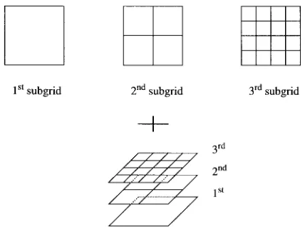
The variable grid consists of a number of different subgrids. Each subgrid is composed of equally sized -dimensional hypercuboids. It implies that the number of the subgrids can increase or decrease with time in the grid according to a design strategy. All subgrids are named, the initial grid is named the first-order subgrid, then the second-order subgrid, and so on. In each subgrid, there are a different number of nodes, which are denoted by their positions. Let denote the set of nodes in the th-order subgrid. Thus, the set of all nodes in the grid with subgrids is
(10)
[image:4.612.325.539.57.216.2]To increase the density of the gridnodes, the edge lengths of the hypercubes of the th-order subgrid will always be less
Fig. 1. Variable grid with three subgrids.
than those of the th-order subgrid. Hence, the higher order subgrids have more nodes than the lower order ones. On the other hand, to reduce the density of the gridnodes, always remove some subgrids from the grid until a required density is reached.
Let all elements of the set represent the possible centers of the network. So, the more subgrids, the more possible centers. Since the higher order subgrids probably have some nodes that are the same as the lower order subgrids, the set of the new possible centers provided by the th order subgrid is defined as
and for
(11)
where is an empty set. It shows that the possible center set corresponding to the th subgrid does not include those that are given by the lower order subgrids, i.e.,
(12)
For example, in the two-dimensional (2-D) case, let the edge length of rectangulars on the th subgrid be half of the th subgrid. The variable grid with three subgrids is shown in Fig. 1.
B. Variable Network
The variable neural network has the property that the num-ber of the basis functions in the network can be either increased or decreased over time according to a design strategy.
For the problem of nonlinear modeling with neural net-works, the variable network is initialized with a small number of basis function units. As observations are received, the network grows by adding some new basis functions or is pruned by removing some old ones.
To add new basis functions to the network the following two conditions must be satisfied: 1) the modeling error must be greater than the required accuracy and 2) the period between the two adding operations must be greater than the minimum response time to the adding operation.
error must be less than the required accuracy and 2) the period between the two removing operations must be greater than the minimum response time of the removing operation.
It is known that if the grid consists of the same size -dimension hypercubes with the edge length vector
, the accuracy of approximating a function is in direct proportion to the norm of the edge length vector of the grid [46], i.e.,
(13)
Therefore, based on the variable grid, the structure of a variable neural network is proposed here. The network selects the centers from the node set of the variable grid. When the network needs some new basis functions, a new higher order subgrid (say, th subgrid) is appended to the grid. The network chooses the new centers from the possible center set provided by the newly created subgrid. Similarly, if the network needs to be reduced, the highest order subgrid (say, th subgrid) is deleted from the grid. Meanwhile, the network removes the centers associated with the deleted subgrid. In this way, the network is kept to a suitable size. How to locate the centers and determine the widths of the GRBF’s is discussed in the next section.
C. Selection of Basis Functions
It is also known that the GRBF has a localization property that the influence area of the th basis function is governed by the center and width . In other words, once the center and the width are fixed, the influence area of the GRBF is limited in the state-space to the neighborhood of .
On the basis of the possible center set produced by the variable grid, there are large number of basis function candidates, denoted by the set . During the system operation, the state vector will gradually scan a subset of the state-space set . Since the basis functions in the GRBF network have a localized receptive field, if the neighborhood of a basis function is located “far away” from the current state , its influence to the approximation is very small and could be ignored by the network. On the other hand, if the neighborhood of a basis function is near to or covers the current state , it will play a very important role in the approximation. Thus, it should be kept if it is already in the network or added into the network if it is not in.
Given any point , the nearest node
to it in the th subgrid can be calculated by
round (14)
for , where round is an operator for rounding the number to the nearest integer; for example, round , and is the edge length of the hypercube
corresponding to the th element of the vector in the th subgrid. Without lose of generality, let
.
Define hyperspheres corresponding to the subgrids, respectively
(15)
for , where is the radius of the th hypersphere. In order to get a suitable-sized variable network, choose the centers of the basis functions from the nodes contained in the different hyperspheres , which are centered in the nearest nodes to in the different subgrids with radius , for . For the sake of simplicity, it is assumed that the basis function candidates whose centers are in the set have the same width and . Thus, for the higher order subgrids, use the smaller radius, i.e.,
(16)
Usually, choose
(17)
where is a constant and less than one. Thus, the chosen centers from the set are given by the set
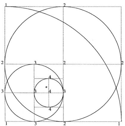
and (18)
In order that the basis function candidates in the set that are less than an activation threshold to the nearest grid node in the th subgrid are outside the set , it can be deduced from (8) and (15) that the must be chosen to be
(19)
for , where represents the
activation threshold.
Thus, the center set of the network is given by the union of the center sets , for , that is
(20)
For example, in the 2-D case, the radii are chosen to be the same as the edge lengths of the squares in the subgrids, that is
for (21)
The chosen centers in the variable grid with four subgrids are as shown in Fig. 2.
Now, consider how to choose the width of the th basis function. The angle between the two GRBF’s and is defined as in (22), shown at the bottom of the
Fig. 2. Location of centers in the variable grid with four subgrids. The numberi (i = 1; 2; 3; 4) denotes the centers chosen from the ith subgrid.
previous page, where is the inner product in the space of square-integrable functions, which is defined as
(23)
The angle can be given by [20]
(24)
where . It shows from the above that the
depends on three factors: the dimension , the width ratio , and the output of a basis function at the center of the other basis function .
If the centers of the two basis functions are chosen from the same subgrid, i.e., , it is clear from (24) that
(25)
On the other hand, if the centers of the two basis functions are from different subgrids, it is possible that their centers are very close. The worst case will be when is near to one. In this case, the angle between the two basis functions can be written as
(26)
Given the center , in order to assign a new basis function that is nearly orthogonal to all existing basis functions, the angle between the GRBF’s should be as large as possible. The width should therefore be reduced. However, reducing increases the curvature of that in turn gives a less smooth function and can lead to overfitting problems. Thus, to make a tradeoff between the orthogonality and the smoothness, it can be deduced from (25) and (26) that
the width , which ensures the angles between GRBF units are not less than the required minimum angle should satisfy
(27)
or
(28)
and
(29)
For example, assume that the satisfies (27). If the width of the basis functions whose centers are located in the set , which corresponds to the th subgrid with , is chosen to be and the width of the basis functions associated to the initial grid satisfies
(30)
then the smallest angle between all basis functions are not less than the required minimum angle .
Therefore, based on a variable grid with subgrids, the nonlinear function approximated by the GRBF network in (6) can also be expressed by
(31) where
(32)
is the th element of the set , is the number of its elements, and and are the optimal weights. So, the next step is how to obtain the estimates of the weights.
IV. ADAPTIVE CONTROL
A. Adaptation Laws
We assume that the basis functions for are given. Section IV-B will discuss how the basis functions of the network model are chosen.
The control objective is to force the plant state vector to follow a specified desired trajectory . The tracking error vector and the weight error vectors, respectively, are defined as
(33)
(34)
(35)
where and are the estimated weight vectors. From (1), it can be shown that
(36)
Hence, from (33)–(36), the dynamical expression of the track-ing error is
(37)
One approach to this problem is to take the control input satisfying
(38)
where the vector makes the following matrix stable:
..
. ... ... ... ... (39)
i.e., all eigenvalues are in the open left plane. The control input consists of a linear combination of the tracking errors , the adaptive part that will attempt to estimate, and cancel, the unknown function , and is a feedforward of the th derivative of the desired trajectory.
Consider the following Lyapunov function:
(40)
where is chosen to be a positive definite matrix so that the matrix is also a positive definite matrix and and are positive constants that will appear in the sequential adaptation laws, also referred to as the learning or
adaptation rates. Using (37), the derivative of the Lyapunov function with respect to time is given by
(41)
where the vector is the th row of the matrix , i.e., .
Since is a constant vector, we have that , similarly, . If there is no modeling error, i.e., , the weight vectors and can simply be generated according to the following standard adaptation
laws: and .
In the presence of a modeling error , to ensure the stability of the system, a lot of algorithms, e.g., the fixed or switching -modification [16], [17], -modification [37], and the dead-zone methods [38], [52], can be applied to modify the above standard adaptation laws.
Define the following sets:
or and
(42)
and (43)
or
and (44)
and (45)
where and are positive constants.
Here, in order to avoid parameter drift in the presence of modeling error, the application of the projection algorithm [11], [15], [45] gives the following adaptive laws for the parameter estimates and , as in (46) and (47), shown at the bottom of the page. It is clear that, if the initial weights
are chosen such that and ,
the weight vectors and are confined to the sets
and , respectively. With use of the adaptive laws (46) and (47), (41) becomes
(48)
For the sake of simplicity, the positive definite matrix is assumed to be diagonal, i.e., , where
, for . Also define
(49)
where is a positive variable, i.e., .
if
if (46)
if
If there is no modeling error (i.e., ), (48) can be written as
(50)
The above clearly shows that is negative semidefinite. Hence, the stability of the overall identification scheme is guaranteed and
(51)
On the other hand, in the presence of modeling error, (48) can be expressed as
(52)
It is easy to show from the above that, if , is still negative and the tracking errors will converge to the set . But, if , it is possible that , which implies that the weight vectors and may drift to infinity over time. The adaptive laws (46) and (47) avoid this drift by limiting the upper bounds of the weights. Thus, the tracking error always converges to the set and the overall control scheme will remain stable in the case of modeling error.
B. Adaptive Control Algorithm
From the set that gives a relationship between the tracking and modeling errors, it can be shown that the tracking error depends on the modeling error. If the modeling error is known, the set to which the tracking error will converge is also known. However, in most cases, the upper bound is unknown.
In practice, control systems are usually required to keep the tracking errors within prescribed bounds, that is
for (53)
where is the required accuracy. At the beginning, it is very difficult to know how many neural network units are needed to achieve the above control requirements. In order to find a suitable-sized network for this control problem, first set lower and upper bounds for the tracking errors, which are functions of time , and then try to find a variable network such that
for (54)
where are monodecreasing functions of time , respectively. Those bounds are usually defined as
(55)
(56)
where are constants and less than one,
are the initial values. It is clear that decrease with time . As approach zero. Thus, in this way, the tracking errors reach the required accuracies given in (53).
According to the relationship between the modeling error and the tracking error, it is easy to know that given the lower and upper bounds of the tracking errors the modeling error corresponding to the above should be
(57)
It is easy to know that the area that the set covers is a hyperellipsoid with the center
(58)
Thus, it can be deduced from the set given by (49) that the upper bound and the lower bound are given by
(59)
(60)
Hence, if the tracking error , the network needs more basis functions. Add the th order subgrid to the grid. The parameters associated with the GRBF units are then changed as follows:
(61)
(62)
(63)
(64)
(65)
(66)
where , for , is a constant and less than one. But, if the tracking error , the network needs to remove some basis functions. Just remove the units associated with the th subgrid. The parameters associated with the GRBF units are then changed as follows:
(67)
(68)
(69)
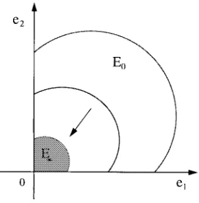
Fig. 3. Two-dimensional convergence area.
parameters. For the 2-D case, the convergence area is shown in Fig. 3. At the beginning, the convergence area of the tracking area is . Finally, it approaches to the expected convergence
area , that is, , for .
V. SIMULATION RESULTS
This section considers two examples. The first is concerned with adaptive control of a time-invariant nonlinear system. The second considers adaptive control of a time-variant nonlinear system.
Example 1: The dynamical system used in the simulation
example is given in [51]
(70)
which is a second-order time-invariant nonlinear system. The parameter values used in this example are as follows: the reference input ; the initial value of the output ; the initial value of the output derivative ; the required accuracy of the tracking error
vector ; the constants ;
the initial values , for
; the required minimum angle between the GRBF’s ; the edge length of the rectangles in the first subgrid is ; the radius of center selection in the first subgrid ; the width of the GRBF units corresponding to the first subgrid ; the activation threshold ; the initial number of the variable networks is 45;
the vector ; the matrix ;
and the adaptation rates and .
The parameters associated with the variable network are
(71)
for . The maximum of (the number of the subgrids) is limited to be 11.
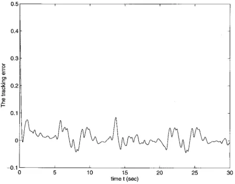
The weights are adaptively adjusted by the laws in (46) and (47). The adaptive control law is given by (38). The results of the simulation are shown in Figs. 4–6. Though the difference between the system output and the desired output is very large at the beginning, the system is still stable and the tracking error asymptotically converges to the expected range, which
[image:9.612.315.550.60.245.2]Fig. 4. Reference inputyd(t), output y(t), reference input derivative _yd(t), and output derivative _y(t) of the system.
Fig. 5. Tracking errory(t) 0 yd(t) of the system.
is also shown in Fig. 5. As it can be seen from Fig. 6, the number of GRBF units in the neural network also converges in a period of time.
Example 2: Consider a time-variant nonlinear dynamical
system given by
(72)
This plant is different from that in Example 1. The functions and in Example 1 are time-invariant nonlinear functions. While, here the functions and are time variant.
[image:9.612.312.552.290.476.2]Fig. 6. NumberK of GRBF units in the variable neural network.
Fig. 7. Tracking errory(t) 0 yd(t) of the system.
neural networks also works well for time-variant nonlinear systems.
VI. CONCLUSION
A variable neural network structure has been proposed, in which the number of the basis functions in the network can be either increased or decreased over time according to some design strategy to avoid either overfitting or underfitting. In order to model unknown nonlinearities of nonlinear systems, the variable neural network starts with a small number of initial hidden units, then adds or removes units on a variable grid consisting of a variable number of subgrids with different sized hypercubes, based on the novelty of observation. The adaptive control algorithm, developed by combining the variable GRBF network and Lyapunov synthesis techniques, guarantees the stability of the control system and the convergence of the tracking errors. The number of GRBF units in the neural network also converges by introducing the monodecreasing upper and lower bounds of the tracking errors. The results of the simulation examples illustrate the operation of the variable neural network for adaptive nonlinear system control.
REFERENCES
[1] C. W. Anderson, “Learning to control an inverted pendulum using neural networks,” IEEE Contr. Syst. Mag., vol. 9, pp. 31–37, 1989.
[2] P. J. Antsaklis, Ed., “Special issue on neural networks in control systems,” IEEE Contr. Syst. Mag., vol. 10, no. 3, 1990.
[3] G. Barto, Neural Network for Control. Cambridge, MA: MIT Press, 1990.
[4] E. Baum and D. Haussler, “What size net gives valid generalization,”
Neural Computat., vol. 1, no. 1, pp. 151–160, 1989.
[5] S. A. Billings and S. Chen, “Neural networks and system identification,” in Neural Networks for Systems and Control, K. Warwick et al., Eds. London, U.K.: Peregrinus, 1992, pp. 181–205.
[6] S. Chen, S. A. Billings, and P. M. Grant, “Nonlinear system identifica-tion using neural networks,” Int. J. Contr., vol. 51, no. 6, pp. 1191–1214, 1990.
[7] S. R. Chi, R. Shoureshi, and M. Tenorio, “Neural networks for system identification,” IEEE Contr. Syst. Mag., vol. 10, pp. 31–34, 1990. [8] S. Fabri and V. Kadirkamanathan, “Dynamic structure neural networks
for stable adaptive control of nonlinear systems,” IEEE Trans. Neural
Networks, vol. 7, no. 5, pp. 1151–1167, 1996.
[9] S. E. Fahlman and C. Lebiere, “The cascade-correlation architecture,” in
Advances in Neural Information Processing Systems 2, D. S. Touretzky,
Ed. San Mateo, CA: Morgan Kaufmann, 1990.
[10] K. S. Fu, “Learning control systems—Review and outlook,” IEEE Trans.
Automat. Control, vol. 16, pp. 210–221, Jan. 1970.
[11] G. C. Goodwin and D. Q. Mayne, “A parameter estimation perspective of continuous time model reference adaptive control,” Automatica, vol. 23, no. 1, pp. 57–70, 1987.
[12] A. Guez, J. L. Elibert, and M. Kam, “Neural network architecture for control,” IEEE Contr. Syst. Mag., vol. 8, pp. 22–25, 1988.
[13] K. J. Hunt and D. Sbararo, “Neural networks for nonlinear internal model control,” Proc. Inst. Elect. Eng. D, vol. 138, pp. 431–438, 1991. [14] K. J. Hunt, D. Sbararo, R. Zbikowski, and P. J. Gawthrop, “Neural networks for control systems—A survey,” Automatica, vol. 28, no. 6, pp. 1083–1112, 1992.
[15] P. A. Ioannou and A. Datta, “Robust adaptive control: Design, analysis and robustness bounds,” in Foundations of Adaptive Control, P. V. Kokotovic, Ed. Berlin, Germany: Springer-Verlag, pp. 71–152, 1991. [16] P. A. Ioannou and P. V. Kokotovic, Adaptive Systems with Reduced
Models. New York: Springer-Verlag, 1983.
[17] P. A. Ioannou and Tsakalis, “A robust direct adaptive control,” IEEE
Trans. Automat. Control, vol. AC-31, pp. 1033–1043, Sept. 1986.
[18] A. Isidori, Nonlinear Control Systems: An Introduction. Berlin, Ger-many: Springer-Verlag, 1989.
[19] A. Karakasoglu, S. L. Sudharsanan, and M. K. Sundareshan, “Identi-fication and decentralized adaptive control using neural networks with application to robotic manipulators,” IEEE Trans. Neural Networks, vol. 4, pp. 919–930, June 1993.
[20] V. Kadirkamanathan, “Sequential learning in artificial neural networks,” Ph.D dissertation, Univ. Cambridge, Cambridge, U.K., 1991. [21] , “A statistical inference based growth criteria for the RBF
network,” in Proc. IEEE Workshop Neural Networks Signal Processing, 1994, pp. 12–21.
[22] V. Kadirkamanathan and G. P. Liu, “Robust identification with neural networks using multiobjective criteria,” in Preprints 5th IFAC Symp.
Adaptive Syst. Contr. Signal Processing, Budapest, Hungary, 1995, pp.
237–242.
[23] V. Kadirkamanathan and M. Niranjan, “Application of an architec-turally dynamic network for speech pattern classification,” in Proc. Inst.
Acoust., 1992, vol. 14, part 6, pp. 343–350.
[24] , “A function estimation approach to sequential learning with neural networks,” Neural Computation, vol. 5, pp. 954–957, 1993. [25] I. D. Landau, Adaptive Control—The Model Reference Approach. New
York: Marcel Dekker, 1979.
[26] G. P. Liu and V. Kadirkamanathan, “Learning with multiobjective criteria,” in Proc. 4th Int. Conf. Artif. Neural Networks, Cambridge, U.K., 1995, pp. 35–40.
[27] G. P. Liu, V. Kadirkamanathan, and S. A. Billings, “Identification of nonlinear systems using growing RBF networks,” in Proc. 3rd Eur.
Contr. Conf., Rome, Italy, 1995, pp. 2408–2413.
[28] , “Stable sequential identification of continuous nonlinear dynam-ical systems by growing RBF networks,” Int. J. Contr., vol. 65, no. 1, pp. 53–69, 1996.
[29] , “Nonlinear predictive control using neural networks,” in Proc.
Control’96, U.K.
[image:10.612.51.288.280.466.2][31] , “On-line identification of nonlinear systems using Volterra polynomial basis function neural networks,” in Proc. 4th Eur. Contr.
Conf., Brussels, Belgium, 1997.
[32] Y. LeCun, J. S. Denker, and S. A. Solla, “Optimal brain damage,” in
Advances in Neural Information Processing Systems 2, D. S. Touretzky,
Ed. San Mateo, CA: Morgan Kaufmann, 1990, pp. 598–605. [33] D. J. C. MacKay, “Bayesian interpolation,” Neural Computat., vol. 4,
no. 3, pp. 415–447, 1992.
[34] T. M. Miller, R. S. Sutton III, and P. J. Werbos (Eds.), Neural Networks
for Control. Cambridge, MA: MIT Press, 1990.
[35] J. Moody and C. J. Darken, “Fast learning in networks of locally-tuned processing units,” Neural Computat., vol. 1, pp. 281–294, 1989. [36] M. C. Mozer and P. Smolensky, “Skeletonization: A technique for
trimming the fat from a network via relevance assignment,” in Advances
in Neural Information Processing Systems 1, D. S. Touretzky, Ed. San Mateo, CA: Morgan Kaufmann, 1989.
[37] K. S. Narendra and A. M. Annaswamy, “A new adaptive law for robust adaptation with persistent excitation,” IEEE Trans. Automat. Contr., vol. 32, no. 2, pp. 134–145, 1987.
[38] , Stable Adaptive Systems. Engelwood Cliffs, NJ, Prentice-Hall, 1989.
[39] K. S. Narendra and K. Parthasarathy, “Identification and control of dy-namical systems using neural networks,” IEEE Trans. Neural Networks, vol. 1, pp. 4–27, Jan. 1990.
[40] H. Nijmeijer and A. J. van der Schaft, Nonlinear Dynamical Control
Systems. New York: Springer-Verlag, 1990.
[41] M. Niranjan and F. Fallside, “Neural networks and radial basis functions for classifying static speech patterns,” Comput. Speech Language, vol. 4, pp. 275–289, 1990.
[42] J. Platt, “A resource allocating network for function interpolation,”
Neural Computat., vol. 4, no. 2, pp. 213–225, 1991.
[43] T. Poggio and F. Girosi, “Networks for approximation and learning,”
Proc. IEEE, vol. 78, pp. 1481–1497, Sept. 1990.
[44] , “Regularization algorithms for learning that are equivalent to multilayer networks,” Science, vol. 247, pp. 978–982, 1990.
[45] M. M. Polycarpou and P. A. Ioannou, “Identification and control of nonlinear systems using neural network models: Design and stability analysis,” Dept. Elect. Eng. Syst., Univ. Southern California, Tech. Rep. 91-09-01, 1991.
[46] M. J. D. Powell, Approximation Theory and Methods. Cambridge, U.K., Cambridge Univ. Press, 1981.
[47] , “Radial basis functions for multivariable interpolation: A re-view,” in Algorithms for Approximation, J. C. Mason and M. G. Cox, Eds. Oxford, U.K.: Oxford Univ. Press, 1987, pp. 143–167. [48] D. Psaltis, A. Sideris, and A. A. Yamamura, “A multilayered neural
network controller,” IEEE Contr. Syst. Mag., vol. 8, pp. 17–21, 1988. [49] S. Z. Qin, H. T. Su, and T. J. McAvoy, “Comparison of four net
learn-ing methods for dynamic system identification,” IEEE Trans. Neural
Networks, vol. 3, pp. 122–130, Jan. 1992.
[50] N. Sadegh, “A perceptron network for functional identification and control of nonlinear systems,” IEEE Transactions Neural Networks, vol. 4, pp. 982–988, June 1993.
[51] R. M. Sanner and J. J. E. Slotine, “Gaussian networks for direct adaptive control,” IEEE Trans. Neural Networks, vol. 3, pp. 837–863, June 1992. [52] S. Sastry and M. Bodson, Adaptive Control: Stability, Convergence and
Robustness. Engelwood Cliffs, NJ: Prentice-Hall, 1989.
[53] J. J. E. Slotine and W. Li, Applied Nonlinear Control. Engelwood Cliffs, NJ: Prentice-Hall, 1991.
[54] P. Smyth, “On stochastic complexity and admissible models for neural network classifiers,” in Advances in Neural Information Processing
Systems 3, R. P. Lippmann, J. Moody, and D. S. Touretzky, Eds. San Mateo, CA: Morgan Kaufmann, 1991.
[55] R. J. Werbos, “Backpropagation through time: What it does and how to do it,” Proc. IEEE, vol. 78, pp. 1550–1560, Dec. 1990.
[56] M. J. Willis, G. A. Montague, C. Di. Massimo, M. T. Tham, and A. J. Morris, “Artificial neural networks in process estimation and control,”
Automatica, vol. 28, no. 6, pp. 1181–1187, 1992.
Guoping P. Liu (M’97) was born in Changsha,
China, in November 1962. He received the B.Eng. and M.Eng. degrees in electrical and electronic engineering from the Central South University of Technology, China, in 1982 and 1985, respectively, and the Ph.D. degree in control systems engineer-ing from the University of Manchester Institute of Science and Technology, Manchester, U.K., in 1992.
He was appointed as a Lecturer in the Department of Automatic Control Engineering, Central South University of Technology, in 1985 and as a Professor in the Institute of Information Engineering, Central South University of Technology, in 1994. He received the Alexander von Humboldt Research Fellowship in 1992. From 1992 to 1993, he worked as a Postdoctoral Research Assistant in the Department of Electronics, University of York, York, U.K. From 1993 to 1996, he was a Research Associate in the Department of Automatic Control and Systems Engineering, University of Sheffield, Sheffield, U.K. He was a Senior Engineer in the Mechanical Engineering Centre, GEC-Alsthom, Leicester, U.K. from 1996 to 1998. He is currently with the ALSTOM Energy Technology Centre, Leicester. He developed an eigenstructure assignment toolbox for use with MATLAB. He is a co-author of three books: Critical
Control Systems: Theory, Design and Applications (New York: Research
Studies Press and Wiley, 1993), Advanced Adaptive Control (Oxford, U.K.: Pergamon, 1995), and Eigenstructure Assignment for Control System Design (Chichester, U.K.: Wiley, 1998). His main research interests include nonlinear system identification and control, adaptive control, eigenstructure assignment for multivariable control systems, multiobjective optimization and control, robust control, critical control systems, and real-time computer control and applications.
Visakan Kadirkamanathan (S’89–M’90) was born
in Jaffna, Sri Lanka, on October 15, 1962. He received the B.A. degree in electrical and informa-tion sciences (with first-class honors) in June 1987 and the Ph.D. degree in February 1992, both from Cambridge University, Cambridge, U.K.
He was a Postdoctoral Research Assistant in the Electrical and Electronic Engineering Depart-ment, University of Surrey, Surrey, U.K., from 1991 to 1992 and in the Engineering Department, Cambridge University. Since 1993, he has been a Lecturer in the Department of Automatic Control and Systems Engineering, University of Sheffield, Sheffield, U.K. His research interests include nonlinear systems, neural networks, adaptive estimation and control, medical signal analysis, engine fault diagnosis, and applications of neural networks.
Stephen A. Billings was born in the United
King-dom in 1951. He received the B.Eng. degree in electrical engineering (with first-class honors) from the University of Liverpool, Liverpool, U.K., in 1972, the Ph.D. degree in control systems engineer-ing from the University of Sheffield, Sheffield, U.K., in 1976, and the D.Eng. degree from the University of Liverpool, Liverpool, U.K., in 1990.
He was appointed Professor in the Department of Automatic Control and Systems Engineering, University of Sheffield in 1990 and leads the Signal Processing and Machine Vision Research Group. His research interests include system identification and signal processing for nonlinear systems, time series analysis, spectral analysis, adaptive noise cancellation, nonlinear systems analysis and design, fault detection, neural networks, machine vision, and brain imaging.