Robust and sparse estimation of large precision matrices

(1)

Robust and Sparse Estimation of Large

Precision Matrices

Ginette Lafit

Doctoral Thesis

Universidad Carlos III de Madrid Department of Statistics

Advisors: Francisco J. Nogales Ruben H. Zamar

(2)

c

(3)

Abstract

The thesis considers the estimation of sparse precision matrices in the high-dimensional setting. First, we introduce an integrated approach to estimate undirected graphs and to perform model selection in high-dimensional Gaussian Graphical Models (GGMs). The approach is based on a parametrization of the inverse covariance matrix in terms of the prediction errors of the best linear predictor of each node in the graph. We exploit the relationship between partial correla-tion coefficients and the distribucorrela-tion of the prediccorrela-tion errors to propose a novel forward-backward algorithm for detecting pairs of variables having nonzero partial correlations among a large number of random variables based on i.i.d. samples. Then, we are able to establish asymptotic properties under mild conditions. Finally, numerical studies through simulation and real data examples provide evidence of the practical advantage of the procedure, where the proposed approach outperforms state-of-the-art methods such as the Graphical lasso and CLIME under different settings.

Furthermore, we study the problem of robust estimation of GGMs in the high-dimensional setting when the data may contain outlying observations. We propose a robust precision matrix estimator under the cellwise contamination mechanism that is robust against structural bivariate outliers. This framework exploits robust pairwise weighted correlation coefficient estimates, where the weights are computed by the Ma-halanobis distance with respect to an affine equivariant robust correlation coefficient estimator. We show that the convergence rate of the proposed estimator is the same as the correlation coefficient used to compute the Mahalanobis distance. We conduct numerical simulation under different contamination settings to compare the graph recovery performance of different robust estimators. The proposed method is then applied to the classification of tumors using gene expression data. We show that our procedure can effectively recover the true graph under cellwise data contamination.

(4)

Acknowledgements

“Kiss me while I calculate and calibrate and heaven’s sake don’t make me explain.”

— Fiona Apple First, I would like to thank Javier Nogales for supervising my thesis. He gave me excellent help and support and was always open for questions. I would like to express my sincere gratitude to Ruben Zamar for his patience, motivation, and immense knowledge. I could not have imagined having better advisors and mentors for my Ph.D study. Their guidance helped me in all the time of research and writing of this thesis. They have the talent of creating a very motivating and reassuring atmosphere that wide my research from various perspectives. Besides, I would like to thank Marcelo Ruiz for his insightful comments, contributions and valuable ideas.

I am grateful to the Department of Statistics of Universidad Carlos III de Madrid, for providing the financial support to carry out this thesis. In particular, I want to show my gratitude to Susana Linares and Francisco Garc´ıa Saavedra for their help and administrative assistance.

Furthermore, I want to thank all my colleagues of the Department of Statistics for creating a familial working environment which made my time at the department truly enjoyable. In particular, I thank Andres Benchimol, Diego Ayma, Mar´ıa Guadarrama and Jorge Herrera for many stimulating discussions.

My time in Madrid was made enjoyable in large part due to the many friends that became a part of my life. I am grateful to my lovely friends: Gisela, Mar, Florinda, Elena and Gabri.

Last but not the least, I would like to thank my family: my parents and to my brother and sister and the rest of the family for their unconditional love and support throughout writing this thesis they have cherished with me every great moment and encourage me to be disobedient and to follow my intuitions.

(5)

(6)

List of Tables

2.1 Graphical Stepwise algorithm. Selected edges in forward and backward step. . . 42

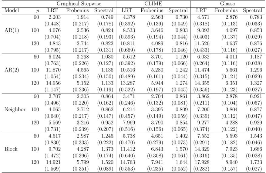
2.2 Comparison of average numerical performance for four models over 100 replications with standard deviation in brackets. . . 54

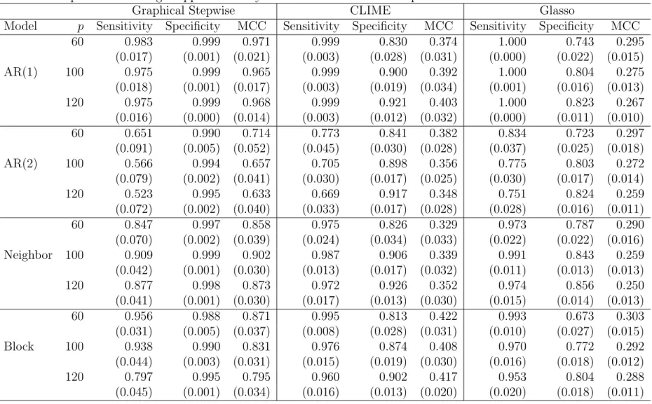
2.3 Comparison of average support recovery for four models over 100 repli-cations with standard deviation in brackets. . . 55

2.4 Comparison of average pCR classification errors over 100 replications with standard deviation in brackets. . . 57

3.1 Estimation performance of the bivariate winsorized correlation coef-ficient under non contamination over 100 replications with standard deviations in brackets. . . 80

3.2 Average computing times (in seconds) over 100 replications with stan-dard deviations in brackets. . . 81

3.3 AR(1)-Model Specification. Numerical performance under the first contamination mechanism over 100 replications with standard devi-ation in brackets. . . 95

3.4 Erd¨os-R´enyi Specification. Numerical performance under the first con-tamination mechanism over 100 replications with standard deviation in brackets. . . 96

(9)

3.5 AR(1)-Model Specification. Numerical performance under the second contamination mechanism over 100 replications with standard devia-tion in brackets. . . 99

3.6 Erd¨os-R´enyi Specification. Numerical performance under the second contamination mechanism over 100 replications with standard devia-tion in brackets. . . 100

3.7 Comparison of average pCR classification errors over 100 replications with standard deviation in brackets. . . 103

3.8 Comparison of average leukemia classification errors over 100 replica-tions with standard deviation in brackets. . . 105

(10)

List of Figures

2.1 Undirected block graph (whenp= 6). Nodes are represented by circles and undirected edges are represented by lines. . . 36

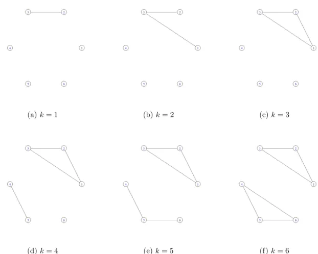
2.2 Graph representation of the estimated undirected graphs in each step of the Graphical Stepwise Algorithm. . . 42

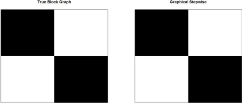
2.3 Heatmaps of the frequency of the zeros identified for each entry of Ω (when p = 6) out of 100 replications. White represents 100 zeros identified out of 100 runs, and black represents 0/100. . . 43

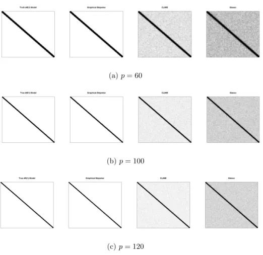
2.4 AR(1) Model. Heatmaps of the frequency of the zeros identified for each entry of Ω out of 100 replications. White represents 100 zeros identified out of 100 runs, and black represents 0/100. . . 50

2.5 AR(2) Model. Heatmaps of the frequency of the zeros identified for each entry of Ω out of 100 replications. White represents 100 zeros identified out of 100 runs, and black represents 0/100. . . 51

2.6 2-nearest-neighbor graph. Heatmaps of the frequency of the zeros iden-tified for each entry ofΩout of 100 replications. White represents 100 zeros identified out of 100 runs, and black represents 0/100. . . 52

2.7 Block graph. Heatmaps of the frequency of the zeros identified for each entry of Ω out of 100 replications. White represents 100 zeros identified out of 100 runs, and black represents 0/100. . . 53

(11)

3.1 Illustration of nonparanormal tranformation and bivariate winsoriza-tion under bivariate contaminawinsoriza-tion. The nonparanormal transforma-tion does not take into account the orientatransforma-tion of the bivariate data. The bivariate data winsorization shrinks points outside an ellipse that connects points of equal Mahalanobis distance (2.45) towards its boundary. . . 79

3.2 AR(1)-Model Specification. ROC curves under the first contamination mechanism over 100 replications. . . 92

3.3 Erd¨os-R´enyi Specification. ROC curves under the first contamination mechanism over 100 replications. . . 93

3.4 AR(1)-Model Specification. ROC curves under the second contamina-tion mechanism over 100 replicacontamina-tions. . . 97

3.5 Erd¨os-R´enyi Specification. ROC curves under the second contamina-tion mechanism over 100 replicacontamina-tions. . . 98

(12)

Chapter 1 Introduction

1.1 Motivation

Many statistical and practical problems require the estimation of different measures of linear dependence to infer whether there exists an association between a pair of variables, when we conditioned on the rest of them. Statistically, this is measured by the partial correlation coefficient. Thus, when two variables are linearly and condi-tionally associated, the partial correlation coefficient is different from zero (Edwards,

2000).

Let x= (X1, ..., Xp)T ∈Rp be a multivariate and centered vector with covariance

matrix Σ and precision matrix Ω = Σ−1. Then, the linear relation between two variables excluding the effect of the others can be measured by the partial correlation coefficient defined as follows:

Definition 1. The partial correlation coefficient between two variables(Xi, Xj),

con-dition on the rest of them and denoted by ρij, is defined as the correlation coefficient

between Xi and Xj when the effect of the other variables is eliminated.

Assuming that the vector x = (X1, ..., Xp)T is multivariate Gaussian distributed

(13)

corre-lation coefficients are closely related with the elements of the precision matrix Ω(see

Lauritzen, 1996). Hence, we can relate the nonzero entries in the precision matrix with the nonzero partial correlation coefficients. This procedure was first proposed by

Dempster (1972) and is denoted by Covariance Selection. Let ωij be the ij-element

of the precision matrix Ω. Then, the partial correlation coefficient between variables

Xi and Xj is given by the following expression:

ρij =−

ωij

[ωiiωjj]1/2

f or i, j= 1, ..., p. (1.1.1) A problem that is closely related with covariance selection is the recovery of the support of the precision matrix (i.e. non-zero elements of Ω). This problem is con-nected with model selection in undirected graphical models. An undirected graph, denoted by G = (V, E) is defined as the set of p vertices, denoted by V, that repre-sents thepvariables and the set of edges, given byE ⊆V ×V. The undirected graph establishes that if the variablesXi andXj are connected, then the pair (i, j)∈E, and

the variables Xi and Xj are adjacent. Furthermore, the edge (i, j) is excluded from

E if and only if Xi and Xj are independent given (Xk, k∈V \ {i, j}). In particular,

if x= (X1, ..., Xp)T is multivariate Gaussian distributed then, the conditionally

inde-pendence between Xi andXj is equivalent toωij = 0. Thus, recovering the structure

of the graph G= (V, E) is equivalent to estimate the non-zero elements inΩ. This is known in the literature as Gaussian Graphical Models (GGMs) (Lauritzen, 1996).

Given an independent and identically distributed random sample{x1, ...,xn}from

the distribution of x, the most natural estimator of Σ is the empirical covariance matrix defined as:

S= 1 n n X k=1 (xk−x)(x¯ k−x)¯ T, (1.1.2) where ¯x = n−1Pn

k=1xk. For data sets in which the ratio between the dimension p

(14)

of the empirical covariance matrix can be used as an estimate forΩ. However, when

p > n, S is not invertible. Moreover, when the ratio p/n is approximately one, S is still invertible but ill-conditioned, meaning that its inverse will amplify the estimation error, which can be observed by the presence of small eigenvalues (Ledoit and Wolf,

2004). Moreover, from the asymptotic point of view, when both n and p are large (i.e. p = O(n)), the empirical covariance matrix is not a consistent estimator (see

El Karoui,2008). Therefore, in the high-dimensional setting, traditional methods that relies on the optimization of a discrete function (Speed and Kiiveri, 1986; Lauritzen,

1996; Edwards, 2000) do not work well due to the lack of a pivotal estimator like the empirical covariance matrix. Hence, different methods focus on obtaining an estimator of Σ that can be inverted and is well-conditioned.

Moreover, in the high-dimensional setting several covariance selection procedures focus on the assumption that the precision matrix is sparse, that is, Ω is mostly composed by zero elements. This suggests that even when we are dealing with p =

O(n), the dimension of the problem may still be tractable since the number of edges will grow slowly than the number of observations (Meinshausen and B¨uhlmann,2006). Sparse Gaussian Graphical Models have been apply to the construction of gene regulatory networks (see Wille et al., 2004; Li and Gui, 2006; Kiiveri, 2011). In the genetic literature, a well known result is that the process in which the cell controls the interaction between RNAs and proteins can be theoretically represented as a network. This approach explores dependence relations between genes through the estimation of the corresponding precision matrix. Moreover, this framework assume that the patterns of variation in gene expressions will be predicted by a small subset of other genes. Hence, genetic networks are not fully connected, suggesting that genetic networks are intrinsically sparse and hence the associated precision matrix is mostly composed by zero elements outside its principal diagonal.

(15)

Finally, We have to note that there is a growing literature onDirect Acyclic Graph-ical Models or Bayesian Networks (see Spirtes et al., 2000; Kalisch and B¨uhlmann,

2007; B¨uhlmann et al., 2010). These are defined as graphical models in which the edges have directional arrows but not directed cycles (see Chapter 2Lauritzen,1996). However, in the present thesis we focus on the estimation of GGM where all edges are undirected. For the remainder of this chapter we review existing approaches to estimate the precision matrix and we present the organization and outline of the thesis.

1.2 Precision Matrix Estimation

Existing methods to estimate undirected GGM in the high-dimensional setting can be classified in two classes: the nodewise regression methods and maximum likeli-hood methods. The nodewise regression method was proposed by Meinshausen and B¨uhlmann (2006). This method estimate for each node in the graph the set of par-tial correlated variables. Penalized likelihood methods include Yuan and Lin(2007),

Banerjee et al. (2008) and Friedman et al. (2008), among others. These methods propose to estimate the precision matrix by penalizing the log-likelihood function.

Notation. Given a vector v ∈ _Rp _{and parameter} _a _∈ _[1_,_∞_{), we use} _k _v _k a to

denote the usual `a norm. We consider k v k1=

Pp

i=1|vi|, k v k2=

pPp

i=1vi2 and k v k∞= maxi|vi|. Given a matrix U= (uij) ∈ Rp×p we define the elementwise `∞

norm k U k∞= max1≤i≤p,1≤j≤p|uij|, the spectral norm k U k2= supkxk2≤1 k Ux k2, the matrix `1 norm k U kL1= max1≤j≤p

Pp

i=1|uij|, the Frobenius norm k U kF=

q P

i,ju

2

ij and the elementwise `1 norm k U k1=

Pp

i=1

Pp

j=1|uij|. The notation

(16)

1.2.1 Estimation by Multiple Regression

The methods that rely on estimation by multiple regression aim to detect pair of vari-ables with non-zero partial correlation based on independent identically distributed samples. Meinshausen and B¨uhlmann (2006) develop a procedure, called Neighbor-hood Selection, that uses lasso penalty (Tibshirani,1996) to estimate the conditional independence structure of a set of variables x = (X1, ..., Xp)T which are Gaussian

distributed with mean zero and covariance Σ. The neighborhood of a variable is defined in the following way:

Definition 2. The neighborhood of a node i ∈ V, denotes by Ai, is the smallest

subset of the set of vertices that not contain the node i (i.e. V \ {i}) such that, given all the nodes in the neighborhood,Xi is conditionally independent of all the remaining

variables that do not belong to the subset Ai.

For each node i∈V, the optimal predictor for Xi,βi ∈Rp, is defined as

βi = arg min β∈Rp,βi=0 kXi− p X j=1 βjXj k22, (1.2.1)

Meinshausen and B¨uhlmann (2006) show that

β_ji =−ωij

ωii

. (1.2.2)

Given an identically and independent distributed random sample {x1, . . . ,xn}, the

Neighborhood Selection approach aims to estimate individually the neighborhood of a variable Xi assuming that the precision matrix Ω is sparse. The Neighborhood

Selection procedure estimates for each node i ∈V the vector of coefficients βi ∈ _Rp

by minimizing the following lasso regression for each variable:

ˆ βi = arg min β∈_Rp_,βi₌₀    n−1 n X k=1 Xki− p X j=1 βjXkj !2 +λ1 kβ k1    , (1.2.3)

(17)

where λ1 >0 is the penalty parameter in the lasso regression and kβ k1=

Pp

j=1|βj|

is the `1 norm of the coefficient vector. Hence, Meinshausen and B¨uhlmann (2006)

define the estimated set of neighborhoods for node i∈V as: ˆ

Ai ={j ∈V : ˆβji 6= 0}, (1.2.4)

Hence, neighborhood selection estimates p separate lasso regressions. The elements of Ω are estimated to be non-zero if ˆβi

j 6= 0 or ˆβ j

i 6= 0. The solution will depend

on the penalty parameter λ1, large values will tend to increase the set of variables

included in the neighborhood, while low values will shrink the set.

Meinshausen and B¨uhlmann (2006) prove that under certain conditions it is pos-sible to estimate consistently the neighborhood of each node in the graph when the dimension grows exponentially as a function of the sample size. Hence, the Neigh-borhood Selection approach has an exponentially fast convergence rate and the con-ditional independence structure of a multivariate Gaussian distribution can be esti-mated consistently by combining the neighborhood estimates for all variables.

The neighborhood selection procedure is a simple method to recover the neighbor-hood of a variable consistently under a set of suitable assumptions. Moreover is also computationally fast for large data sets. However, it does not take into account the intrinsic symmetry of Ω. This could produce a loss in efficiency and contradictory neighborhoods. Also, the same penalty is used for all the p lasso regressions, which is only efficient when the distribution of the network is nearly uniform (Peng et al.,

2009).

Peng et al. (2009) develop a procedure, calledSparse Partial Correlation Estima-tion (SPACE), that is based on a joint sparse regression model that simultaneously perform neighborhood selection and preserves symmetry. SPACE can detect pairs of variables that have non-zero partial correlations among a large number of random

(18)

variables based on independent identically distributed samples with mean zero and covariance matrixΣ. Using the fact thatXi can be expressed asXi =P_j6=iβ

i

jXj+εi,

such that εi is uncorrelated withX−i, we can write βji in terms of the coefficients of

the precision matrix Ω:

β_ji =−ωij ωii =ρij r ωjj ωii , (1.2.5)

where ρij is the partial correlation coefficient and ωij the coefficients of the precision

matrix Ω.

Given this result, Peng et al. (2009) define the following loss function

Ln(θ,Ω,X) = 1 2   p X i=1 wi n X k=1 Xki− X j6=i ρij r ωjj ωii Xkj !2 , (1.2.6)

where θ= (ρ12, ..., ρ(p−1)p), ω={ωii}pi=1,X ={xk}nk=1 and w={wi}pi=1 are

nonneg-ative weights.

The partial correlation vector θ= (ρ12, ..., ρ(p−1)p) is estimated by minimizing the

following penalized loss function

L(θ,ω,X) = Ln(θ,ω,X) +λ2 kθk1, (1.2.7)

where λ2 is the regularization parameter andkθ k1=P₁≤i<j≤p|ρij|is an `1 penalty.

There are three different types of weights that can be considered: (1) uniform weights , wi = 1, (2) residual variance based weights wi = ˆωii and (3) degree based

weights, where wi is proportional to the estimated degree of Xi (i.e. this is related

with the number of variables such that ˆρij 6= 0 for j 6=i).

Peng et al.(2009) show that under certain conditions the SPACE method produces consistent estimates and can identify the correct neighborhood when both n → ∞ and p→ ∞.

(19)

1.2.2 Penalized Maximum Likelihood

Under the assumption that x = (X1, ..., Xp)T are normally distributed with mean

µ and covariance Σ. The objective of the following procedures is to estimate the precision matrixΩ imposing some type of penalization on the likelihood function to control the number of zeros in the precision matrix.

Yuan and Lin (2007) propose a method to estimate sparse graphical models. As-suming that the data is multivariate Gaussian, a `1 penalty is imposed on the

likeli-hood function to estimate Ω. Therefore, the objective is to maximize the following

`1 regularized log-likelihood function:

max Ω0 ( log|Ω| −tr(SΩ)−λ3 p X i=1 p X j=1 |ωij| ) . (1.2.8)

where λ3 >0 is the regularization parameter.

From the optimization problem in (1.2.8), we can define the sub-gradient equation for minimizing the log-likelihood

W−S−λ3Λ= 0, (1.2.9)

where W = Ω−1, Λij ∈ sign(ωij) (i.e. Λij = sign(ωij) if ωij 6= 0 and Ωij = 0 if

Λij ∈[−1,1]).

Given that the problem in (1.2.8) is convex, Banerjee et al. (2008) consider the estimation of the covariance matrix Σ. Assuming that W is an estimate of Σ, they show that the solution can be obtained by optimizing over each row and corresponding column of W in a block coordinate descending fashion. To illustrate the idea, if the matrix W and S are partitioned in the following way

W=    W11 w12 wT₁₂ w22    S =    S11 s12 sT₁₂ s22   ,

(20)

the solution forw12 is given by:

w12 = arg min

y

yTW−₁₁1y:ky−s12k∞≤λ3 . (1.2.10)

Which is identical to solve the following dual problem:

w12=m βin 1 2kW 1/2 11 β−bk 2₊_λ 4kβk1 , (1.2.11)

where b =W−₁₁1/2s12. Consequently, if β solves the problem in (1.2.11) then w12 =

W11β solves equation (1.2.10).

Friedman et al. (2008) state that the problem in (1.2.11) resembles a lasso re-gression and is similar to the first order condition, given by equation (1.2.9), when optimizing the log-likelihood imposing and `1 penalty. To illustrate the similarities

between the two approaches, we can partition Wand Ω in the following way:

WΩ=    W11 w12 wT₁₂ w22       Ω11 ω12 ωT₁₂ Ω22   =    I(p−1) 0(p−1)×p 0p×(p−1) 1   . (1.2.12)

The sub-gradient equation (1.2.9) can be written in terms of the elements of the partition matrices as

w12−s12−λ4γ12= 0. (1.2.13)

Given the result in Banerjee et al. (2008) we can conveniently write the problem in (1.2.13) as a lasso regression problem:

W11β−s12+λ4v= 0, (1.2.14)

(21)

If we setW11=S11, the estimates of the problem in (1.2.8) are the same to those

proposed by Meinshausen and B¨uhlmann (2006), in which a lasso regression is fitted to each of the p variables taking as regressors the rest (p−1) variables. However,

Banerjee et al.(2008) show that this approach does not yield the maximum likelihood estimator, since in general W11 6= S11. Therefore, to solve this problem, Friedman

et al. (2008) propose a new algorithm, the Graphical Lasso or Glasso, that uses an estimate of the upper block ofWinstead of using S11 directly. The Glasso algorithm

works in the following manner:

1. Start with W = S + λ4Ip. The diagonal of W remains unchanged in the

following steps.

2. For each j = 1,2, ..., p,1,2, ..., p, ... solve the Lasso problem in (1.2.11), that takes as input the inner products W11 and s12. This gives a (p−1) vector of

solutionβb. Fill in the corresponding row and column of Wusingw₁₂ =W₁₁βb.

3. Continue until convergence.

Step 2 implies a permutation of the rows and columns to make the target column the last. Thus each lasso problem can be efficiently solved by a coordinate descent algorithm (see Friedman et al., 2008). Since, the estimated βb will be sparse the

computation ofw12=W11βbwill be fast. The Glasso algorithm will estimateΣb =W,

and the precision matrix can be recovered solving the system of equations in (1.2.12). A disadvantage of the Graphical lasso algorithm is that the `1 penalty tends to

produce biases even in the simple regression setting, due to the linear increase of penalty on regression coefficients. Fan et al. (2009) propose two different procedures to remedy this situation, one of them relies on non-concave penalties, the Smoothly Clipped Absolute Deviation (SCAD), and the other is theAdaptive Lasso.

Fan and Li(2001) consider that a good penalty function should be able to produce and estimator with three properties: (1) the estimator should be unbiased when the

(22)

true parameter is large to avoid unnecessary modeling bias. (2) It should produce sparsity, this implies that the resulting estimator is a thresholding rule which auto-matically sets small estimated coefficients to zero to reduce model complexity. (3) The resulting estimator should be continuous in data to avoid instability in model prediction. Fan and Li (2001) and Fan et al. (2009) show that these properties are achieved by the SCAD penalty, which is symmetric on a quadratic spline [0,∞) where the first order derivative is given by

SCAD0_λ 5,a =V n I(|x|< λ5) + (aλ5− |x|)+ (a−1)λ5 o , (1.2.15)

forx≥0, whereλ5 >0 anda >2 are two tuning parameters. Whena → ∞equation

(1.2.15) corresponds to the `1 penalty. This penalty function leaves large values of

|x| not excessively penalized and makes the solution continuous. Using the SCAD penalty, the optimization problem is given by

max Ω0 ( log|Ω| −tr(SΩ)− p X i=1 p X j=1 SCADλ5,a(|ωij|) ) . (1.2.16)

Fan and Li (2001) demonstrate that the rates of convergence for the penalized likeli-hood estimators depend on the regularization parameter. While for the `1 penalized

likelihood the oracle property does not hold, the SCAD penalty performs as well as the oracle procedure in terms of selecting the correct model.

Another procedure that achieves the three properties mention before is the Adap-tive Lasso penalty (Zou,2006), which set a different weight to each component, thus the problem is to optimize the following restricted log-likelihood function:

max Ω0 ( log|Ω| −tr(SΩ)−λ6 p X i=1 p X j=1 wij|ωij| ) , (1.2.17)

(23)

wherewij = 1/|ωeij|

γ _{for some}_{γ >}_{0 and any consistent estimator}

e

Ω= [ω_eij]1≤i,j≤p, the

initial estimates of Ωe can be obtained by estimating the precision matrix applying a

lasso penalty.

The SCAD penalty is a more flexible approach than the Adaptive Lasso, since an element being estimated zero can escape from zero in the next iteration. While the Adaptive Lasso absorbs zeros in each iteration producing estimates that are always sparser than the initial values (see Fan et al.,2009).

Finally, another method that considers the dual problem of optimizing a`1

penal-ized likelihood function to estimate Ω is developed byCai et al. (2011) and denoted by Constrained `1-minimization for Inverse Matrix Estimation (CLIME). Let Ωb1 to

be the solution of the following optimization problem:

minkΩk1 subject to |ΣΩ−I |∞≤λ7 Ω∈Rp×p, (1.2.18)

where λ7 is a tuning parameter. This problem does not impose the symmetry

con-dition on Ω, thus the solution, _bω1

ij, is not symmetric. Therefore, the final CLIME

estimator of the precision matrix is obtained in the following way:

b ωij =ωbji =bω 1 ij1(|ωb 1 ij |≤bω 1 ij) +ωb 1 ji1(|ωb 1 ij |>ωb 1 ij). (1.2.19)

This implies that between ω_b1

ij and ωb

1

ji, the one that is selected is the one with the

smallest magnitude. The method will also guarantee that Ωb is positive definite.

Cai et al. (2011) prove that the rate of convergence of CLIME outperforms the rates of convergence for`1Penalized Maximum Likelihood estimators and also satisfies

that kΩb −Ωk2=Op r log p n ! . (1.2.20)

(24)

1.3 Robust Precision Matrix Estimation

One of the main drawback of the popular procedures to estimate the precision matrix is that they are not well suited to handle noisy data (contaminated by outliers). The existing approaches to estimate the precision matrix and recover the support of the GGM use as input the empirical covariance matrix. The empirical covariance and correlation matrix estimates are very sensitive to the presence of multidimensional outliers (Alqallaf et al., 2002). The violation of the Gaussian assumption may re-sult in poor recovery of the GGM and biased estimation of the precision matrix (see

Finegold and Drton, 2011; Liu et al., 2012; Sun and Li, 2012). Moreover, in the high-dimensional setting, the fraction of perfectly observed rows may be very small. If all components of a row have an independent chance of being contaminated, then the probability that a case is perfectly observed is small. To deal with outliers in the high-dimensional setting,Alqallaf et al.(2009) propose a contamination model where the contamination in each variable is independent from other variables (i.e. compo-nentwise outliers). It allows for cellwise contamination that can be applied to explain the contamination mechanism in Microarrays experiments (see Troyanskaya et al.,

2001;Liu et al.,2003). The cellwise contamination model lacks the affine equivariant property. Henceforth, existing approaches for robust covariance estimation such as M-estimates (Hampel,1973;Maronna,1976), Minimum Volume Ellipsoid (MVE) and Minimum Covariance Determinant (MCD) estimators (Rousseeuw, 1985, 1984) and the Stahel-Donoho (SD) estimators (Stahel,1981;Donoho,1982), may not be reliable in high-dimensional data sets.

To deal with outliers in high-dimensional data sets, many procedures construct robust covariance and correlation matrices by using pairwise robust correlation coeffi-cients. Liu et al.(2009) andLiu et al.(2012) propose to apply a univariate monotone transformation to make the data Gaussian distributed. Then, a robust precision es-timator of the correlation matrix can be computed from the transformed data. The

(25)

main drawback of these procedures is that they are not robust under the presence of structural bivariate outliers which could lead to a misleading graph support recovery.

1.4 Organization and Outline of the Thesis

The thesis is structure as follows. In Chapter 2 we present an approach to esti-mate undirected graphs and to perform model selection in high dimensional Gaussian Graphical Models. We consider a parametrization of the precision matrix in terms of the prediction errors of the best linear predictor of each node in the graph. We exploit the relationship between partial correlation coefficients and the distribution of the prediction errors. We propose a novel forward-backward algorithm for detect-ing pairs of variables havdetect-ing nonzero partial correlations among a large number of random variables based on i.i.d. samples. We establish asymptotic properties under mild conditions. The proposed algorithm outperforms the existing methods, such as the Graphical lasso and CLIME, when we compare the graph recovery and numerical performance under different settings. Numerical studies through simulation and real data examples provide evidence of the theoretical advantage of the procedure.

Chapter 3 is concerned with robust estimation of Gaussian Graphical Models in the high-dimensional setting when the data may contain outlying observations. These outliers can lead to drastically wrong inference on the intrinsic graph struc-ture. Several procedures apply univariate transformations to make the data Gaussian distributed. However, these transformations do not work well under the presence of structural bivariate outliers. We propose a robust precision matrix estimator un-der the cellwise contamination mechanism that is robust against structural bivariate outliers. This estimator exploits robust pairwise weighted correlation coefficient esti-mates, where the weights are computed by the Mahalanobis distance with respect to an affine equivariant robust correlation coefficient estimator. We show that the

(26)

con-vergence rate of the proposed estimator is the same as the correlation coefficient used to compute the Mahalanobis distance. We conduct numerical simulation under dif-ferent contamination settings to compare the graph recovery performance of difdif-ferent robust estimators. Finally, the proposed method is then applied to the classification of tumors using gene expression data. We show that our procedure can effectively recover the true graph under cellwise data contamination. Chapter 4 concludes the thesis.

(27)

Chapter 2 A Stepwise Approach for

High-Dimensional Gaussian

Graphical Models

High-dimensional Gaussian Graphical models (GGMs) have been widely used to rep-resent the linear dependency between variables. The idea underlying GGMs is to measure linear dependencies by estimating partial correlations to infer whether there is an association between a pair of variables, conditionally on the rest of them. More-over, there is a close relation between the nonzero partial correlation coefficients and the nonzero entries in the inverse of the covariance matrix (Lauritzen,1996;Edwards,

2000). This procedure is known as covariance selection and is widely used to iden-tify the conditional independence in an undirected graph from a set of independently indentically distributed observations (Dempster, 1972).

In a high-dimensional framework, when the dimensionpis larger than the number of available observations n, the sample covariance matrix is badly conditioned and its inverse tends to amplify the estimation error (Ledoit and Wolf, 2004). From the asymptotic point of view, when both n and p are large (i.e. p = O(n)), the sample

(28)

covariance matrix is not a consistent estimator (El Karoui,2008). To deal with this problem, several covariance selection procedures have been proposed based on the assumption that the inverse of the covariance matrix (i.e. precision matrix) is sparse. This implies that most of the variables are conditionally independent.

Existing methods to estimate the GGM can be classified in three classes: the nodewise regression methods, maximum likelihood methods and limited order partial correlations methods. The nodewise regression method was proposed byMeinshausen and B¨uhlmann (2006). This method estimate a lasso regression for each node in the graph. Peng et al. (2009) present a procedure that simultaneously performs neigh-borhood selection for all variables to estimate joint sparse regressions, applying an active-shooting to solve the lasso. Yuan (2010) replaces the lasso regression with a Dantzig selector. Liu and Wang(2012) propose an asymptotically tuning-free proce-dure that estimates the precision matrix in a column-by-column fashion. Zhou et al.

(2011) propose an estimator for the precision matrix base on `1 regularization and

thresholding to infer a sparse undirected graphical model. Ren et al.(2015) propose a nodewise regression approach to obtain asymptotically efficient estimation of each entry of the precision matrix under sparseness conditions.

Penalized likelihood methods includeYuan and Lin(2007),Banerjee et al. (2008) and Friedman et al. (2008), among others. These methods propose to estimate the precision matrix by penalizing the log-likelihood function. Friedman et al. (2008) propose the Graphical lasso (Glasso) procedure to estimate sparse precision matrices fitting a modified lasso regression to each variable and solving the problem by a co-ordinate descent algorithm. Rates of convergence under the Frobeniuos norm were study byRothman et al.(2008). Ravikumar et al.(2008) andRavikumar et al.(2011) obtain convergence rates under the elementwise `∞ norm and the spectral norm

as-suming subgaussian distributions. Lam and Fan(2009) andFan et al.(2009) propose methods to diminish the bias imposed by the`1 penalty by introducing a non-convex

(29)

SCAD penalty. Cai et al. (2011) propose an estimator called CLIME that estimate precision matrices for both sparse and non-sparse graphs, without imposing a specific sparsity pattern, by solving the dual of an `1 penalized maximum likelihood

prob-lem. They establish convergence rates under the elementwise`∞ norm and Frobenius

norm. A greedy forward-backward algorithm to optimize a Gaussian log-likelihood loss was proposed by Johnson et al. (2011). This algorithm starts with an empty set of active variables and adds (and removes) variables to the active set. In doing so they use a greedy coordinate ascent algorithm, this implies optimizing a quadratic function for every pair of nodes in each iteration. They show that the greedy algo-rithm requires a restricted eigenvalue condition on the true precision matrix. This condition is weaker than the irrepresentable condition impose by the `1 regularized

log-likelihood methods (see Ravikumar et al., 2011).

Limited order partial correlation procedures use lower order partial correlations to test for conditional independence relations. Spirtes et al. (2000) propose the PC-algorithm, which works in an iterative procedure, it starts with a complete undirected graph and deletes edges based on conditional independence decisions. This algorithm works in the worst case in exponential time, but under sparsity assumptions the com-putational complexity is reduced to polynomial time. Kalisch and B¨uhlmann (2007) andR¨utimann et al.(2009) modify the PC-algorithm to estimate direct acyclic graphs. However, their approach has a large degree of computational complexity. Liang et al.

(2015) propose an equivalent measure of partial correlations based on the Markov property and adjacency faithfulness to estimate partial correlation coefficients. Huang et al. (2016) propose a partial correlation screening approach that uses a screen step and a clean step. In the screen step, the algorithm select a reduce neighborhood set for each node using a stagewise algorithm. In the clean step, the algorithm removes false positives and uses the resultant neighborhood set to reconstruct each row of the precision matrix.

(30)

In this article, we present an approach to estimate partial correlations and to per-form model selection in high dimensional Gaussian Graphical Models (GGM) based on a forward-backward algorithm. Our method is motivated by the relation between the partial correlation coefficients and the elements of the precision matrix. We pro-pose to parametrize the precision matrix in terms of the prediction errors of the best linear predictor of each variable. Hence, we convert the original problem of estimating the precision matrix into that of the covariance matrix estimation. We estimate the edge set applying a forward-backward algorithm. The algorithm begins with an empty edge set and gradually adds and removes edges from the edge set. In the forward step the algorithm finds the best next candidate given by the pair of variables with the largest absolute empirical partial correlation coefficient, otherwise the algorithm terminates. In the backward step the algorithm removes the unlikely edges. The max-imization of this coefficient is related to the maxmax-imization of a empirical information divergence measure. We the call this procedure Graphical Stepwise. Compare with existing methods, our approach is able to provide a set of edges associated with the largest absolute partial correlation coefficients for a given threshold. Moreover, under mild conditions we show that the Graphical Stepwise procedure is able to consistently estimate the true set of edges.

The rest of the chapter is organized as follows. In the next section we present a parametrization of the precision matrix which exploits the relation between the elements of the precision matrix and a system of linear regressions. In Section2.2 we present the Graphical Stepwise procedure to estimate a set of edges with a forward-backward algorithm. In Section 2.3 we establish the consistency of the proposed approach. Section2.4presents simulation results and real data analysis. We compare the numerical and classification performance of the method with that of Glasso and CLIME. In Section 2.5 we conclude the article with a brief discussion. Proof of the main results are presented in Section 2.6.

(31)

2.1 Undirected Graphical Models

To make the manuscript self-contained, we first introduce some definitions and ana-lytical results for Graphical Models. Suppose that x = (X1, . . . , Xp)T is a p-variate

random vector with joint distribution F. The conditional independence structure of the distribution can be represented by a graphical model G = (V, E), where

V = {1, . . . , p} is the set of nodes and E ⊆ V ×V the set of edges. The graph is called undirected when all the edges are undirected. If two nodesiand j ∈V form and edge, then i and j are adjacent or neighbors (Lauritzen, 1996; Edwards, 2000). Definition 3. LetG = (V, E)be an undirected graph. The set of neighbors of a node

i∈V is denoted as Ai and is defined by the following set of nodes:

Ai ={k∈V \ {i}: (i, k)∈E}. (2.1.1)

Associated with and undirected graph G and the probability distribution F we can assume a range of different Markov properties. If I ⊆V let XI ={Xi :i∈I}.

Definition 4. (Pairwise Markov Property) We say that F satisfies the Pairwise Markov property (P) with respect to an undirected graph G, if for any pair of un-connected nodes (i, j)∈/E

Xi Xj |XV\{i,j}.

Definition 5. (Local Markov Property) We say that F satisfies the Local Markov property (L) with respect to an undirected graph G, if for any node i∈V

Xi XV\(Ai∪{i})|XAi.

A stronger notion is the Global Markov property. Let I, J, S three disjoint and nonempty subsets of V. We denote XI XJ | XS when XI is independent of XJ

(32)

conditioned on XS; the set S is said to separate I from J if for every node i∈I and

j ∈J, all paths from i to j have at least one node in S. We introduce the following definition.

Definition 6. (Global Markov Property) The probability distribution F satisfies the Global Markov property (G) with respect to G if for every triplet of disjoint and nonempty subsets of nodes I, J, S it holds that XI XJ | XS whenever S

sepa-rates I and J in G.

The three Markov properties are related as follows.

Proposition 1. For any undirected graph G and any probability distribution F, it holds that

(G)=⇒(L)=⇒(P).

The following theorem states that ifF has a positive and continuous density func-tion with respect to a product measure then the Markov properties are all equivalent (see Lauritzen,1996).

Theorem 1. (Pearl and Paz,1985) IfF has a strictly positive and continuous density function with respect to a product measure, then

(G)⇐⇒(L)⇐⇒(P).

A special class of undirected graphical models is the conditionally independence graph. This is a graphical model with undirected graphGand probability distribution

F where the pairwise Markov property holds. Hence, if (i, j) ∈/ E then Xi Xj |

(33)

2.1.1 Gaussian Graphical Models

Suppose that x= (X1, . . . , Xp)T has a joint Gaussian distribution with mean µ=0

and p×p covariance matrix Σ = (σij)i,j=1...,p and let G = (V, E) be the associated

graphical model . If Σ is regular then Ω= (ωij)i,j=1...,p denote the precision matrix

Σ−1.

Consider Xi and Xj with i < j and let xi,j = (Xi, Xj) T

and x−{i,j} the random

vector containing the rest of the variables (the indexes in V \ {i, j} in ascending order) and let x0−{i,j} ∈ R(p−2)×1 be a (fixed) vector. By Proposition C.5. of

Lau-ritzen (1996), the conditional distribution of xi,j given x−{i,j} =x0−{i,j} is normally

distributed with covariance matrix Σi,j|−{i,j} given by the inverse of the matrix

Ai,j =    ωii ωij ωji ωjj   . Hence

Σi,j|−{i,j} =A−_i,j1 =

1 ωiiωjj−ωijωji    ωjj −ωij −ωji ωii   . (2.1.2)

By the normality, conditionally to x−{i,j} = x0−{i,j}, Xi and Xj are independent if

and only ifωij =ωji= 0 (hereafter, for the sake of simplicity, we will omit the vector

x0−{i,j}).

The partial correlation between variables Xi and Xj, ρij, is defined as the

cor-relation coefficient of the conditional distribution of x{i,j} given x−{i,j} and so, by

(2.1.2),

ρij =

−ωij

[ωiiωjj]

1/2 (2.1.3)

and, as a consequence, the following proposition is established (see Proposition of 5.2 of Lauritzen, 1996).

(34)

Proposition 2. (Conditional Independence) Assume that x= (X1, . . . , Xp)T is

mul-tivariate Gaussian distributed with regular covariance matrix Σ. Then, it holds that ∀i, j ∈V, with i6=j:

Xi Xj |XV\{i,j} ⇐⇒ωij = 0 (2.1.4)

or, equivalently,

(i, j)∈/ E ⇐⇒ωij = 0. (2.1.5)

Note that, since the joint Gaussian density function is positive and continuous, as a result of applying Theorem 1the GGMs also satisfies Local and Global Markov properties.

We are interested to express partial correlation in terms of regression coefficients. Let x−i ∈ R(p−1)×1 the random vector with the set of indexes V \ {i} in ascending

order,

Σ−i,−i = Cov (x−i,x−i) (2.1.6)

Σi,−i = Cov (Xi,x−i)

= Cov (Xi,x−i) = (Cov (Xi, X1), . . . ,Cov (Xi, Xi−1))

and Σ−i,i= Cov (x−i, Xi).

Note that, by the same proposition Proposition C5 of Lauritzen (1996), the con-ditional distribution of Xi |x−i satisfies

Xi |x−i ∼N µi|−i,Σi|−i

, (2.1.7)

(35)

Then, for each node i∈ V the optimal predictor for Xi, βi, given the remaining

variables is defined as (see Meinshausen and B¨uhlmann,2006):

βi = argmin β∈Rp:βi=0 kXi− p X j∈V βjXj k22 = argmin β∈_Rp_:_βi₌₀ EXi|x−i Xi− X j∈V βjXj !2 . (2.1.8)

The following Lemma summarizes very well known properties related to multi-variate normal distribution and its proof is given in Section 2.6.

Lemma 1.

a) For every node i∈V the optimal predictor for Xi, βi ∈Rp, satisfies

β_ji =−ωij

ωii

,∀j 6=i (2.1.9)

and β_ii = 0 (by definition).

b) Given i, j ∈ V, the partial correlation ρij is related to βji by the following

ex-pression

ρij =sign(βji)

q

β_ijβi

j. (2.1.10)

c) For every i∈V, Xi satisfies the following regression model

Xi =

X

j6=i

β_jiXj +εi =βixT−i+εi

where β_ji is given by (2.1.9)and the error term εi ∼N 0,Σi|−i

is independent of x−i.

(36)

As a simple consequence of the previous Lemma the errors vectorε = (ε1, . . . , εp) T

has a N (0,Ψ) distribution with Var(εi) and Cov(εi, εj) given by

ψi,i =ω−ii1 and ψi,j =ωij/(ωiiωjj), (2.1.11)

respectively.

As a generalization of equation (2.1.8), for a every node i and Ai ⊆ V \ {i} the

optimal prediction of Xi given the set of variables {Xk:k ∈ Ai} is characterized by

the vector βi,Ai _(see _{Meinshausen and B¨}_uhlmann_, ₂₀₀₆_{) by}

βi,Ai ₌ _argmin β∈Rp:βj=0,∀j /∈Ai kXi− X j∈V βjXj k22 = argmin β∈_Rp_:_βj₌₀_,_∀_{j /}_∈A i E Xi− X j∈V βjXj !2 . (2.1.12)

2.1.2 Inverse Covariance Estimation

Let x = (X1, . . . , Xp)T ∼ N (0,Σ), where Σ is the covariance matrix, Ω = Σ−1 the

precision matrix and let G = (V, E) be the associated graphical model as before. Let {x1, . . . ,xn}be a random sample of the random vector xwherexk = (xk1, . . . , xkp)

T

,

k = 1, . . . , n. Let X= (x1, . . . ,xn)T ∈Rn×p be the data matrix.

In gaussian graphical models (GGMs) we are interested in recovering, based onX, the underlying graph structure and this problem corresponds to determining which off-diagonal entries of Ω are non-zero. Considering (2.1.5) and (2.1.9)

E ={(i, j) :ωij 6= 0}=

(i, j) :β_ji 6= 0 .

The neighborhood of a node i∈V is defined as

(37)

and, in consequence, the estimation of the inverse covariance matrix is equivalent to the estimation of the set of neighborhoods of the nodes i∈V.

As we mentioned in the introduction when p > n the sample covariance matrix is badly conditioned and its inverse tends to amplify the estimation error. For large precision matrix estimationFan et al.(2016) proposed the innovated scalable efficient estimation (ISEE) breaking the large-scale precision matrix estimation into smaller-scale linear regression problems. In the following we give a brief explanation of ISEE. Consider the linear transformation, termed as innovation (in time series litera-ture),

e

x=Ωx (2.1.14)

and note that the unobservablep−variate random vector_exhas a N(0,Ω) distribution. If A, B are subsets of V define (the sub–matrix of Ω)ΩA,B= (ωij)i∈A,j∈B and for

A=B letΩA=ΩA,A. Consider a partition (Al)L_l₌₁ of the set of nodes and, for every

Al, let xAl be the sub–vector ofx formed by its components with indexes in Al. So,

by the definition of _exwe can write the sub–vector x_eAl as

e xAl =ΩAlηAl with η_A l = xAl +Ω −1 AlΩAl,Ac

l. Note now that the result in (3.1.6) can be

general-ized to xAl|xAc l ∼ N −Ω −1 AlΩAl,Ac l,Ω −1 Al

suggesting the following multivariate linear regression model

xAl =CAlxAcl +ηAl (2.1.15)

whereCAl is a matrix of regression coefficients andηAl is the vector of model errors.

Equation (2.1.15) suggest to fit this model and to propose, using some regression technique, an estimate _bη_Al consideringη_Al as a residual vector.

Hence, ΩAl can be estimated by the inverse of the sample covariance matrix,

b

(38)

b

xAl = Ωb_Al_bη_Al. By stacking all these sub-vectors (x_e_Al)

L

l=1 together it is possible to

estimate the oracle innovated vector _ex.

We will briefly discuss below the implementation of the ISSE that will use in our forward-backward method in the next section. Given X = (x1, . . . ,xn)T ∈ Rn×p the

data matrix, the oracle empirical matrix Xe ∈ Rn×p is defined as, (see Fan et al.,

2016),

e

X=XΩ. (2.1.16)

If A is a subset of the set of nodes V, using matrix notation, the model (2.1.15) can be written

XA=CAXAc+E_A (2.1.17)

whereXA,XAc are the sub–matrices ofX with columns inAandAc respectively,E_A

is an n× |A| model error matrix with rows as i.i.d. copies of _bηT_A. The corresponding matrix Xe_A can be written as

e

XA=ΩAEA.

Note now that for every node i ∈ A, it is possible to define the univariate linear regression model for response Xi (ithe column of X) given by the linear regression

Xi =XAcβi+E_i (2.1.18)

where Ei is the corresponding column of the matrix EA and βi ∈ R(p−|A|)×1 is the

column of the regression coefficients matrix CA.

As we mentioned before, using some technique regression we obtain an estimation,

b

βi, of theβi coefficients and so

b Ei =Xi−XAcβbi and E_b_A= b Ei i∈A (2.1.19)

(39)

This equations give a natural estimate, Ωb_A, of the sub–matrix Ω_A defined by b ΩA= n−1Eb T AEb_A −1 (2.1.20)

and so, a plug-in estimator for the unobservable sub–matrix Xe_A isEb_AΩb_A.

When A ranges the partition (Al)Ll=1 we obtain the estimate Xb of the the oracle

empirical matrix Xe and an initial estimate Ωb of the precision matrix Ω:

b X =Xb_Al 1≤l≤L and Ωb = 1 nXb T b X (2.1.21)

To estimate the regression coefficients, ISEE introduced by Fan et al. (2016) use penalized least square with the scale Lasso. Sun and Zhang (2012) show that under mild regularities conditions, the residual error and the regression coefficients, esti-mated with the scaled lasso, are consistent and asymptotically normal. However, this may result in a dense network, thus the final sparse precision matrix estimator is computed by thresholding the elements of n−1_XˆT_Xˆ ₍_{Bickel and Levina}_, _2008a_).

To show that the lasso can consistently estimate the neighborhood of each node, we need to assume the irrepresentable condition and the beta-min condition on the size of the minimal absolute value of non-zero regression coefficients (seeMeinshausen and Bühlmann, 2006; Zhao and Yu, 2006; van de Geer and Bühlmann, 2009; Bühlmann and Van De Geer, 2011). This assumption may be restricted, hence we proposed an alternative approach to estimate the oracle empirical matrix ˜X without resorting to

`1 regularization procedures.

In the next section we propose a non-regularized greedy forward-backward algo-rithm to recover the graph structure and this technique is based, partially, in the estimation of the precision matrix based on innovation although our method use least square regression.

(40)

For each node i ∈ V, the optimal predictor βi,Ai ₌ _βi _{based on the variables}

in the neighborhood set Ai was defined in (2.1.12). Let βb

i

the estimated coefficient vector and letEbi be the estimated residual error of the best predictor ofXi given the

variables in the neighborhood set

b Ei =Xi− p X j=1 b β_jiXj. (2.1.22) By (2.1.20) if Ωb_i = n−1Eb T

i Eb_i and if Xb ∈ Rn×p denotes the estimator of the oracle

empirical matrix X, the estimate of thee i-th element of the oracle empirical matrix e

X is

b

Xi =EbiΩbi fori∈V. (2.1.23)

The estimator of the precision matrix Ω is the sample covariance matrix of the esti-mate oracle empirical matrix

b

Ω=n−1Xb

T

b

X. (2.1.24)

So, for an undirected graphG = (V, E), if we can efficiently recover the support ofΩ supp(Ω) ={{i, j} ∈V : (i, j)∈E}, (2.1.25) then we can estimate the precision matrix as the sample covariance matrix of a random vector that depends on the residuals of the best linear predictor for each node and, so, supp(Ω) can be estimated by supp(Ω).b

2.2 The Proposed Method

In this section, we present a new forward-backward greedy algorithm to recover the structure of a GGM. This procedure estimates, sequentially, the oracle empirical

(41)

matrix and as a consequence obtains an estimation of the precision matrix. We call this procedure Graphical Stepwise.

The algorithm begins with an empty set of edges (i.e. ˆE(0) =∅ where the super-scripts denotes the number of steps). Moreover, the initial neighborhoods sets are given by ˆA(0)_i = ∅ for each i ∈ V. In the forward step, the initial optimal edge is given by the pair of variables with the largest absolute empirical correlation:

(i∗, j∗) = argmax

(i,j)∈( ˆE(0)₎c

|Cor(Xd i,Xj)|. (2.2.1)

The edge set and the neighborhood sets are updated as: ˆE(1) ← {(i∗, j∗)}, ˆA(1)_i∗ ←

{j∗}and ˆA(1)_j∗ ← {i∗}. Next, the algorithm setsk=k+1 and estimates the prediction

errors of Xi∗ and X_j∗ using the result in (2.1.12). If the corresponding absolute

empirical correlation is smaller or equal to a threshold γ (i.e. |Cor(Xd _i∗,X_j∗)| ≤ γ),

the algorithm stops and outputs the current estimate set of edges.

At step k, the current edge set is given by ˆE(k−1). In the forward step, the procedure finds the edge that maximizes the absolute value of the empirical partial correlation coefficient which is define as the empirical correlation coefficient between the estimated prediction errors Eb

(k−1)

i and Eb

(k−1)

j of the best linear predictors of Xi

and Xj based on the set of variables in the neighborhood sets ˆA

(k−1) i and ˆA (k−1) j , respectively for (i, j)∈( ˆE(k−1)₎c_: b ρ(_ijk−1) =Cor(d Eb (k−1) i ,Eb (k−1) j ). (2.2.2)

Then the best next candidate is given by the pair of nodes with the largest absolute empirical partial correlation coefficient:

(i∗, j∗) = argmax (i,j)∈( ˆE(k−1)₎c |Cor( ˆd E (k−1) i ,Eˆ (k−1) j )|. (2.2.3)

(42)

Next, the edge set and the neighborhood sets are updated as ˆE(k) ←Eˆ(k−1)∪{(i∗, j∗)}, ˆ A(_ik∗) ← Aˆ (k−1) i∗ ∪ {j∗} and ˆA (k) j∗ ← Aˆ (k−1)

j∗ ∪ {i∗}. If the corresponding absolute

empirical partial correlation is smaller than γ, the algorithm stops and outputs the current estimate set of edges. Otherwise, the algorithm sets k =k+ 1 and estimates the prediction errors of Xi∗ and X_j∗ using the result in (2.1.12) assuming that the

neighborhood sets are given by ˆA(_i∗k) and ˆA

(k)

j∗ . In the backward step, the algorithm

eliminates the unlikely edges in E(k)_{. Thus, the procedure selects the pair of nodes}

from the edge set with the minimum absolute empirical partial correlation coefficient:

(i∗, j∗) = argmin (i,j)∈( ˆE(k)₎ |Cor( ˆd E (k) i ,Eˆ (k) j )|, (2.2.4)

if the corresponding absolute empirical partial correlation corresponding to nodes (i∗, j∗) is smaller than γ, the algorithm removes the pair of variables from the edge

set: Ê(k−1) ← Eˆ(k) − {(i∗, j∗)}, Â(k −1) i∗ ← Aˆ (k) i∗ − {j∗} and Â (k−1) j∗ ← Aˆ (k) j∗ − {i∗}.

Algorithm 1 summarizes the Graphical Stepwise procedure to learn the structure of a GGM.

The Graphical Stepwise procedure outputs the estimated set of edges, denoted by ˆ

E and the corresponding prediction errors ˆEi for i ∈ V. To estimate the precision

matrix we convert the original problem of estimating Ω into that of a covariance estimation problem. Let ˆX∈_Rn×p _{be the estimator of the oracle empirical matrix ˜}_X

define in (2.1.16). The diagonal elements of ˆΩ are computed as ω_bii =n−1Eb

T

iEbi, and

the estimate of the i-th element of the oracle empirical matrix ˜X is

b

Xi =Eb_iΩb_i fori∈V. (2.2.5)

The estimator of the off-diagonal elements of the precision matrixΩare given by the covariance of the oracle empirical matrix estimate for all pairs of nodes that belong

(43)

to the estimated set of edges ˆE: ˆ ωij =n−1Xˆ T iXˆj (i, j)∈Eˆ ˆ ωij = 0 (i, j)∈/ Eˆ (2.2.6)

The Graphical Stepwise procedure is able to estimate an undirected graph that contains the set of edges with the largest absolute empirical partial correlations coeffi-cients for a given threshold. Also, it is possible to introduce previous knowledge when we construct the network. For instance, if we have information that some variables are conditionally independent we can exclude them from the candidate set of edges

ˆ

E. Moreover, we can reduce the candidate set of edges by performing a correlation screening proposed byFan and Lv (2008). We propose to obtain a reduce candidate set of edges by thresholding the empirical correlation matrix by a constant ξ > 0. Then, the set of candidate edges is defined as follows

ˆ

Eξ ={(i, j) :|Cor(Xd _i,X_j)|> ξ, i, j = 1, . . . , p}. (2.2.7)

Luo et al.(2014) andLiang et al.(2015) show that for an appropriate choice ofξ, the true set of edges is contained in the candidate set of edges ˆEξ with high probability,

(44)

Algorithm 1:Graphical Stepwise algorithm for Gaussian covariance estimation

input : X, Stopping Thresholdγ >0

output:Edge Set Estimation ˆE, Residual Error Estimation ˆEifori∈V

InitializeEˆ(0)_{← ∅}_,Aˆ(0)_i ← ∅,Eˆ(0)i ←Xi fori∈V,k←1;

whiletrue do

Forward Step;

(i∗, j∗)←argmax₍_i,j₎∈( ˆE(k−1)₎C |Cor( ˆd E (k−1) i ,Eˆ (k−1) j )|; ˆ E(k)_←_Eˆ(k−1)_{∪ {}₍_i∗_{, j}∗₎_}_; ˆ A(_i∗k)←Aˆ(k −1) i∗ ∪ {j∗}; ˆ A(_jk∗)←Aˆ (k−1) j∗ ∪ {i∗}; if|Cord( ˆE (k−1) i∗ ,Eˆ(k −1) j∗ )|≤γthen break end ˆ βi∗ _{= argmin} β∈Rp:βl=0,l∈V\Aˆ(_ik∗) kXi∗−Pp l=1βlXlk22 ; ˆ E(_ik∗)=Xi∗−Pp l=1βˆ i∗ l Xl; ˆ βj∗ _{= argmin} β∈Rp:βl=0,l∈V\Aˆ(_jk∗) kXj∗−Pp l=1βlXlk22 ; ˆ E(jk∗)=Xj∗−Pp l=1βˆ j∗ l Xl; k←k+ 1; whiletrue do Backward Step;

(i∗, j∗)←argmin₍_i,j₎∈Eˆ(k−1)|Cor( ˆd E (k−1) i ,Eˆ (k−1) j )|; if|Cord( ˆE (k−1) i∗ ,Eˆ (k−1) j∗ )|≤γthen break end ˆ E(k−1)_←_Eˆ(k)_{− {}₍_i ∗, j∗)}; ˆ A(_ik−1) ∗ ←Aˆ (k) i∗ − {j∗}; ˆ A(_jk−1) ∗ ←Aˆ (k) j∗ − {i∗}; ˆ βi∗_{= argmin} β∈Rp:βl=0,l∈V\Aˆ(i∗k−1) kXi∗− Pp l=1βlXlk22 ; ˆ E(ik∗−1)=Xi∗− Pp l=1βˆ i∗ l Xl; ˆ βj∗_{= argmin} β∈Rp:βl=0,l∈V\Aˆ(j∗k−1) kXj∗− Pp l=1βlXlk22 ; ˆ E(jk∗−1)=Xj∗− Pp l=1βˆ j∗ l Xl; k←k−1; end end

(45)

2.2.1 The Proposed Method: Relation with the Information

Divergence Measure

The Kullback-Leibler information divergence between two densities f and g for the random vector x is defined as

I(f;g) = Ef [log (f(x)/g(x))]

where Ef denotes expectation with respect to the densityf (see Whittaker,2009, pp.

87–104).

Let x, y and z be random vectors with joint density function fx,y,z and let fy|x

and fz|x the densities of the conditional distribution of y |x and z |x, respectively;

let fx be the density function of the vector x. The information (Inf) in y about z

conditional on x is defined by

Inf y z|x=I fx,y,z;fz|xfy|xfx

and it represents a measure of the average amount of information infx,y,zagainst the

independence of y and z conditional on x because Inf y z|x = 0 if and only if y z|x.

Letx= (X1, . . . , Xp)T be a random vector with multivariate Gaussian distribution

and let G = (V, E) be its graphical model. For a fixed pair of nodes i, j consider xi,j = (Xi, Xj)T and x−{i,j} (the random vector containing the rest of the variables)

defined in Subsection 2.1.1.

The following proposition claims that information divergence for measuring the conditional independence of a pair of random variablesXiandXj, given the remaining

(46)

variables). Although its proof is a consequence of Proposition 6.4.6 of Whittaker

(2009) we give a straightforward proof for this particular case.

Proposition 3. For every i, j ∈V it holds Inf Xi Xj |x−{i,j} =−1 2log(1−ρ 2 ij), (2.2.8)

where ρij is the partial correlation coefficient between variablesXi andXj conditioned

on x−{i,j}.

Let x1, . . . ,xn be a random sample xand let Cor( ˆd E

(k−1)

i ,Eˆ

(k−1)

j ) be the empirical

partial correlation coefficient defined as the empirical correlation coefficient between the estimated prediction errors Eb

(k−1)

i and Eb

(k−1)

j of the best linear predictors of Xi

and Xj based on the set of variables in the neighborhood set ˆA

(k−1)

i and ˆA

(k−1)

j .

Lemma 1 relates the correlation between the regression errors and partial coefficient regression and Proposition3establishes the relation with the information divergence. Hence, by the previous considerations, at stepk the Graphical Stepwise algorithm select the pair of nodes (i∗, j∗) that satisfies

(i∗, j∗) = argmax (i,j)∈( ˆE(k−1)₎C −1 2log(1−Cor( ˆd E (k−1) i ,Eˆ (k−1) j )2). (2.2.9)

So, at step k the algorithm select the pair (i∗, j∗) with largest absolute empirical partial correlation coefficient or largest empirical divergence information.

(47)

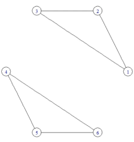
Figure 2.1: Undirected block graph (when p = 6). Nodes are represented by circles and undirected edges are represented by lines.

2.2.2 The Proposed Method: Example

The technique proposed in Section2.2 will now be illustrated numerically on the 6×6 precision matrix Ω: Ω=                 1.0 0.5 0.5 0.0 0.0 0.0 0.5 1.0 0.5 0.0 0.0 0.0 0.5 0.5 1.0 0.0 0.0 0.0 0.0 0.0 0.0 1.0 0.5 0.5 0.0 0.0 0.0 0.5 1.0 0.5 0.0 0.0 0.0 0.5 0.5 1.0                 (2.2.10)

This is a block graphG = (V, E) where the set of nodes are given byV ={1,2,3,4,5} and the set of edges is given by E = {(1,2),(1,3),(2,3),(4,5),(4,6),(5,6)}. The graphical representation is shown in Figure 2.1.

We now show how the Graphical Stepwise procedure works. In doing so, we draw

n = 100 independent samples from a multivariate Gaussian distribution with mean zero and covariance matrixΣ=Ω−1. To select the threshold γ we follow the scheme

(48)

proposed by Cai et al. (2011). We generate a training sample of size n = 100 from a multivariate Gaussian distribution with mean zero and covariance matrix Σ= Ω−1, and an independent sample of the same distribution for validating the thresholding parameter. From the training data, we apply Algorithm 1 for 50 different values of

γ. The optimal parameter is given by the one that minimize the log-likelihood loss defined by:

−log(det( ˆΩ)) + tr( ˆΩXTX)−p. (2.2.11) We replicate each simulation experiment 100 times.

First, we show how the algorithm works in each step for an specific replication where the thresholding parameter is set to γ = 0.165. The algorithm is initialized at stepk= 0 assuming that all variables are conditionally independent. The initial set of edges is ˆE(0) ₌_∅_{and the the initial neighborhoods sets are given by ˆ}_A(0)

i =∅fori∈V.

The initial residual errors are given by ˆE(0)_i =Xi fori∈V. The empirical correlation

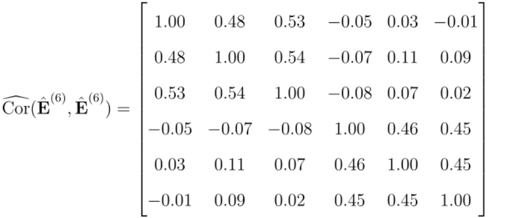
matrix of the estimated residual errors is computed as the empirical correlation matrix of X: d Cor( ˆE(0),Eˆ(0)) =                 1.00 −0.28 −0.37 0.03 −0.01 −0.06 −0.28 1.00 −0.38 −0.11 0.08 0.10 −0.37 −0.38 1.00 −0.06 0.05 −0.00 0.03 −0.11 −0.06 1.00 −0.33 −0.30 −0.01 0.08 0.05 −0.33 1.00 −0.31 −0.06 0.10 −0.00 −0.30 −0.31 1.00                 (2.2.12)

In the forward step, the initial optimal edge is given by the pair of variables with the largest absolute empirical correlation. From the result in (2.2.12), we observe that the largest absolute partial correlation is given by the ordered pair (i∗, j∗) = (2,3) with |Cor( ˆd E

(0) 2 ,Eˆ

(0)

3 )|= 0.38. Given that the corresponding absolute empirical correlation

(49)

the neighborhood sets are updated as: ˆE(1) ₌ _{₍₂_,₃₎_}_{, ˆ}_A(1)

2 ={3} and ˆA (1)

3 = {2}.

The prediction errors of X2 and X3 are estimated using the result in (2.1.12). The

empirical correlation matrix of the estimated residual errors at step k = 1 is given by: d Cor( ˆE(1),Eˆ(1)) =                 1.00 −0.45 −0.51 0.03 −0.01 −0.06 −0.45 1.00 0.38 −0.15 0.11 0.11 −0.51 0.38 1.00 −0.11 0.09 0.04 0.03 −0.15 −0.11 1.00 −0.33 −0.30 −0.01 0.11 0.09 −0.33 1.00 −0.31 −0.06 0.11 0.04 −0.30 −0.31 1.00                 (2.2.13)

In the backward step, the algorithm eliminates the unlikely edges in E(1)_{. Thus, the}

procedure selects the pair of edges from the edge set with the minimum absolute partial correlation. Since the absolute empirical partial correlation of the edge (2,3) is not smaller thanγ, we do not eliminate the edge.

Next, we add an additional edge. In the forward step we select the ordered pair of nodes with the maximum absolute correlation between the empirical residuals in (2.2.13). Which is given by (i∗, j∗) = (1,3). Given that |Cor( ˆd E

(1) 1 ,Eˆ

(1)

3 )| = 0.51 is

larger than γ, The algorithm keeps running. Then, we set k = 2 and the edge set and the neighborhood sets are updated as: ˆE(2) ₌ _{₍₁_,₃₎_,₍₂_,₃₎_}_{, ˆ}_A(2)

1 = {3} and

ˆ

A(2)₃ = {1,2}. The prediction errors of X1 and X3 are estimated using the result in