Text analysis for email multi label classification

(1)

Text analysis for email multi label

clas-sification

Master’s thesis in Computer science and engineering

SANJIT HARSHA KADAM

KYRIAKI PANISKAKI

Department of Computer Science and Engineering CHALMERSUNIVERSITY OF TECHNOLOGY

(2)

(3)

Master’s thesis 2020

Text analysis for email multi label classification

SANJIT HARSHA KADAM

KYRIAKI PANISKAKI

Department of Computer Science and Engineering

Chalmers University of Technology University of Gothenburg

(4)

Text analysis for email multi label classification SANJIT HARSHA KADAM

KYRIAKI PANISKAKI

Supervisor: Marwa Naili, Department of Computer Science and Engineering Advisor: Berenice Gudino, Bokio

Examiner: Devdatt Dubhashi, Department of Computer Science and Engineering

Master’s Thesis 2020

Chalmers University of Technology and University of Gothenburg SE-412 96 Gothenburg

Telephone +46 31 772 1000

(5)

Text analysis for email multi label classification SANJIT HARSHA KADAM

KYRIAKI PANISKAKI

Chalmers University of Technology and University of Gothenburg

Abstract

This master’s thesis studies a multi label text classification task on a small data set of bilingual, English and Swedish, short texts (emails). Specifically, the size of the data set is 5800 emails and those emails are distributed among 107 classes with the special case that the majority of the emails includes the two languages at the same time. For handling this task different models have been employed: Support Vector Machines (SVM), Gated Recurrent Units (GRU), Convolution Neural Net-work (CNN), Quasi Recurrent Neural NetNet-work (QRNN) and Transformers. The experiments demonstrate that in terms of weighted averaged F1 score, the SVM outperforms the other models with a score of 0.96 followed by the CNN with 0.89 and the QRNN with 0.80.

Keywords: natural language processing, machine learning, multi label text classifi-cation, deep neural networks, bilingual texts, emails, short texts.

(6)

(7)

Acknowledgements

We would like to thank our supervisor, Marwa Naili, for the continuous feedback, for guiding us and helping us to accomplish this master thesis within the stipulated time. Moreover, we would like to thankBerenice Gudino, machine learning engineer at Bokio, for her feedback and guidance by helping us overcome and solve our difficulties. Finally, we would like to thank the company Bokio for giving us this opportunity and providing us with the equipment.

(8)

(9)

List of Figures

2.1 Machine learning (Original figure from [32]) . . . 5

2.2 Anatomy of a neural network (Original figure from [32]) . . . 7

2.3 An unrolled Recurrent Neural Network (Original figure from [13]) . . 8

2.4 LSTM architecture (Original figure from [13]) . . . 8

2.5 Bidirectional LSTM architecture (Original figure from [2]) . . . 9

2.6 The attention mechanism (Original figure from [23]) . . . 9

2.7 Gated Recurrent Units (Original figure from [6]) . . . 10

2.8 CNN framework (Original figure from [63]) . . . 11

2.9 Computation structure of the QRNN (Original figure from [29]) . . . 13

2.10 Structure of a transformer (Original figure from [23]) . . . 15

3.1 Pipeline flowchart . . . 19

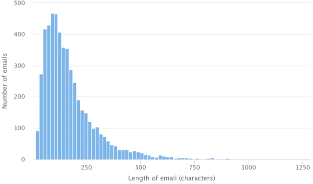
4.1 A histogram demonstrating the length of the emails . . . 23

4.2 Email distribution across classes . . . 24

4.3 Emails with multiple classes . . . 24

4.4 GRU training and validation loss . . . 28

4.5 Very deep CNN training and validation loss . . . 29

4.6 QRNN training and validation loss . . . 31

(12)

(13)

List of Tables

2.1 Confusion matrix (Original table from [50]) . . . 16

3.1 Architecture overview of deep learning models . . . 21

4.1 Classes description . . . 25

4.2 SVM classification report . . . 26

4.3 GRU classification report . . . 27

4.4 Very deep CNN classification report . . . 29

4.5 QRNN classification report . . . 30

4.6 Transformers classification report . . . 32

(14)

(15)

1

Introduction

Natural Language Processing (NLP) is a field of artificial intelligence, which deals with a computer’s ability to understand and process lingual data. The field of NLP encompasses various tasks such as sentiment analysis, text classification, speech recognition or synthesis and semantic analysis. In today’s world, companies exploit a lot of applications of NLP in order to provide and automate services such as machine translation [62], parts of speech tagging [53] or resume (CV) parsing [27].

A process with a main focus on the sorting and transformation of a text into structured, easily manageable data is calledtext analysis and it relies on NLP tech-niques. Text analysis includes multiple tasks such as the prediction of the next word in an email [7], smart replies for incoming messages [21], automated answers for questions based on the content [20] and so on. A common task in the field of text analysis is the multi class text classification problem. Multi class classification refers to the categorization of a sample of input text into one and only one category out of a given set of classes, which contains at least three classes. A more challenging task however, is the multi label classification. In this case, each input data-point can be classified into more than one class at once. This problem requires a model that is more capable of understanding relationships between features in the input text and the output labels for all the classes that are presented.

1.1

Purpose and challenges

This master’s thesis focuses on themulti label text classificationproblem onbilingual short texts (emails). The input data set is in English and Swedish, has a size of 5272 emails, there are 107 classes and it is provided my the company Bokio. The task of the trained model, classifier, will be to assign the proper label(s), out of 107 classes, for each input email. The final model will be used by the company Bokio for tagging the incoming emails automatically. Currently, this procedure is being performed manually by the customer support team at the company.

Most of the existing work on NLP, concerns texts that are written in the English language. That means that handling texts in Swedish is a challenge for this master’s thesis, especially when the same email contains English and Swedish words at the same time. Actually, the majority of the emails contains the two languages and the same time, which also complicates the preprocessing step. Furthermore, the classifier will handle emails which usually are short texts. Shortness, sparseness and lack of contextual information in short texts are the reasons for degrading the classifier’s efficiency. Another major issue is the distribution of the emails among

(16)

1. Introduction

the classes. The total number of the classes are 107 but for some of those classes there are only a few samples which means that the results for those classes will not be efficient. Moreover, this master’s thesis deals with a limited data set of only 5800 examples and this fact will raise the difficulty level. Therefore, the bilingual nature, the short length of the input examples and the relatively small size of the unbalanced data set will be the main field of focus and research contribution of this master’s thesis.

1.2

Approach

In the machine learning field there are various approaches for dealing with a multi label classification task. The majority of those approaches rely on deep learning, which employs artificial neural networks to resolve the task. Long Short Term Memory [49] and Convolutional Neural Networks [34] have been used for multi class text classification tasks. Additionally, Recurrent Neural Network [42] and Transformers [30] have been employed for multi label text classification tasks.

After a comprehensive investigation on the multi label classification problem and based on the performance of the models, four deep learning models will be developed for this master’s thesis. Those models are based on Gated Recurrent Units (GRU), Convolutional Neural Network (CNN), Quasi-Recurrent Neural Network (QRNN) and Transformers. Additionally, to those deep learning models, a more simple model will be developed which relies on support vector machines and it will be used as baseline for comparing the results of the deep learning models with it.

1.3

Roadmap

This master thesis starts with Chapter 2, which describes the theory and the key components of the models that will be used for solving the multi label text classifica-tion task. Chapter 3 presents a step by step descripclassifica-tion of the concrete architecture of the final developed models. Chapter 4 exhibits the results of each model and Chapter 5 includes a discussion and concludes this master’s thesis.

(17)

2

Theory

There are multiple models which can handle and resolve a multi label text classi-fication task. However all the different models rely on three basic steps which are 1) data preparation, 2) model application and 3) evaluation. The next sections de-scribe some data preparation approaches, some machine learning and deep learning classifiers as well as the metrics for evaluating the classifier’s results.

2.1

Data preparation

Text preprocessing is a crucial step of the classification pipeline which takes place at the very beginning of the whole procedure. It is responsible for transforming the input text into a form that is more digestible to enable the classification algorithms to perform better. Text cleaning and data representation aim to increase the efficiency of the classifier.

2.1.1

Text cleaning

The general steps that are taken while preprocessing a piece of input text involve steps such as the removal of extra white spaces, HTML tags, special characters, numbers, proper nouns, conversion of all text into lower case and so on [1]. The main preprocessing techniques that have been used to cleanup and prepare the input before passing it to the models to train are lemmatization and stemming.

Lemmatization

Lemmatization refers to the process of bringing every word in the input dataset back to its root form or ’lemma’ [19]. This groups together sets of words that are the inflected form of the same ’lemma’. These inflections can be in the form of superlatives, plurals, changed tenses and so on. This process assesses the intended part of speech that each word in the input text belongs to and hence, its intended meaning to reduce it down to its ’lemma’ form. The most commonly used package for lemmatization in the English language is the NLTK Lemmatizer. In the case words that are in Swedish however, a system of lemmatization was developed where each word is taken back to its root form by comparing it to a pre-built reference database that is built on a Swedish thesaurus. An example of how lemmatization works is that the Swedish word bokförs (posted) will be transformed into bokföra (post).

(18)

2. Theory

Stemming

Stemming refers to the process of reducing inflected words in a piece of text back to their root (word stem) form [19]. The results from stemming however mean that the root word of a particular set of words need not necessarily be a valid word that belongs to the lexicon of the corresponding language. It just ensures that related words map to the same root word or stem. The most commonly used stemmer for the English language is the NLTK stemmer. For the Swedish language, the most commonly used one is the Snowball Stemmer in the same NLTK library. An exam-ple of stemming is the word anpassade (customized), which will be used as anpass (adaptation).

2.1.2

Text representation

The data should be transformed into a format so that the model can understand and handle them. The machine learning algorithm expects numbers as input, which means that the text should be converted into numbers. For this task the steps are 1) tokenization and 2) vectorization. The step tokenization refers to how the texts will be divided into words or subtexts or n-grams. This determines the "vocabulary" of the data set, which is constituted by unique tokens. The step vectorization is this one which transforms the tokens into numerical vectors. Below are presented some vectorization techniques [22].

One-hot encoding

For each token of the vocabulary a unique index is assigned. Then each sample text is represented as a vector indicating the presence (symbolized by 1) or absence (symbolized by 0) of a token in the text.

Count encoding

In the case of count encoding the vector indicates the count of the tokens in the text.

TF–IDF encoding

Stands for term frequency–inverse document frequency and implies the relative fre-quency of words in a specific document compared to the inverse proportion of that word over the entire document corpus. TF-IDF determines how relevant a token is in a sample [55].

Word Embedding

In this case the meaning of the word is taken into account. The vector of each text represents the location and distance between words indicating how similar they are semantically.

Once the text representation has been accomplished the next step is the feature selection. After having determine the tokens the vocabulary might be too large and some of those tokens (features) might not contribute to the label prediction. Feature selection is responsible to measure how much each token contributes to label predictions and for this purpose there are some statistical functions. One example

(19)

2. Theory

is the function f_classif, which calculates the feature importance [5].

2.2

Machine learning in text classification

In classical programming developers give the rules and data in a program and the program produces the answers. With machine learning developers provide the data and the answers and the outcome is the rules, Figure 2.1. A machine learning system is trained rather than programmed [32]. The most popular machine learning algorithms that are used for text classification are presented in the next sections.

Figure 2.1: Machine learning (Original figure from [32])

2.2.1

Naive Bayes

Probabilistic modeling is the application of statistics to data analysis. One of the most popular algorithms is the Naive Bayes algorithm which relies on Bayes the-orem. Applying the theorem assigns to each class the probability that a sample belongs to the specific class [32]. In paper [37] the authors have presented a mod-ified version of Naive Bayes for text classification with unbalanced classes. Their approach significantly improved the area under the ROC curve (Receiver Operating Characteristic, which illustrates the diagnostic ability of a classifier [15]).

2.2.2

Support vector machines

Support vector machines (SVM) belong to kernel methods and aim at solving clas-sification problems by finding good decision boundaries between two sets of points belonging to two different categories. SVMs are widely used in natural language processing. At the University of Amsterdam a team of researchers utilizes struc-tural Support Vector Machine (SVM) in order to tackle the hierarchical multi label classification task of social short text streams [57]. In [24] the authors studied the multi label text classification in Arabic and they presented a problem method which relies on SVM and achieved 71% ML-accuracy.

2.2.3

Random forest

Random forest is an ensemble decision tree algorithm that builds large numbers of decision trees and then ensembles their outputs [47]. An interesting contribution to

(20)

2. Theory

Random Forests is being described in [28] where the authors present their approach for handling a short text classification task. By enriching the data semantically and then applying Random Forests, they increased the accuracy by 34%.

2.2.4

Gradient boosting machines

A gradient boosting machine behaves much like a random forest, which means that it is based on assembling decision trees. It uses gradient boosting, which improves any machine learning model by training new models that specialize in addressing the weak points of the previous models. Gradient boosting machines outperforms random forests most of the time [32].

2.2.5

Logistic regression

Logistic regression is an algorithm which is based on the concept of probability and there are many applications in the text classification domain. In [47] the authors presented their results for classifying violent events taking place in South Africa on event detection using WhatsApp messages. They experimented with SVM, random forest, gradient boosting and logistic regression and they found that the logistic classifier achieved a 0.899 accuracy against the second best model which was the SVM with 0.895 accuracy.

2.3

Deep learning in text classification

Deep learning is a subfield of machine learning that relies on the artificial neural networks and learns representation from data through the use of successive layers of increasing representation stacked in neural networks that are learnt simultaneously [32]. Deep learning offers better performance on many problems. Moreover, with machine learning the developers had to manually find good layers of representations for the data. This is called feature engineering and deep learning automates this step.

A neural network has some key components which constitute it’s anatomy as figure 2.2 depicts. Those components are:

• Layers which are combined into a network.

• Loss function which measures how far the output is from the expected value. • Optimizer which helps the network to update itself based on the data it sees

and its loss function.

Initially, the weights have random values, the output is far from the expected value and the loss score is high. The network starts processing the samples (text input), the weights are adjusted a little in the correct direction and the loss score decreases. A network with a minimal loss is one for which the outputs are as close as they can be to the targets and is called trained network.

For handling a text classification task one more important key component is the last layer activation. The activation function constrains the network’s output. For a text classification task the predicted values should be between 0 and 1. The most

(21)

2. Theory

popular activation functions for this purpose are sigmoid, relu and softmax, where the sigmoid function is the most suitable for a multi label text classification problem.

Figure 2.2: Anatomy of a neural network (Original figure from [32])

Deep learning has a crucial impact on natural language processing and the deep models have become the new state of the art methods for NLP problems [63]. Long Sort Term Memory networks offered improvements on machine translation [60], [38] and language modeling [43]. Convolutional Neural Networks used for sentence classi-fication [45] or for extracting sentiment, emotion and personality features for sarcasm detection [54]. Transformers have been used for document encoding and summa-rization [65].

2.3.1

Recurrent Neural Networks

The Recurrent Neural Network (RNN) is a neural sequence model that achieves state of the art performance on tasks such as language modeling, sequential labeling or prediction [64]. RNNs are recurrent in nature as they perform the same function for every input data while the output of the current input depends on the hidden state from the previous time step as well. This means that, in other neural networks all the inputs are independent of each other, but in the case of RNNs, the inputs are related to each other through hidden states.

2.3.1.1 Model

An RNN model consists of an input layer, a hidden layer and an output layer. The aspect that makes this network different from a vanilla artificial neural network is the fact that it is time dependant. This means that the input vector to every time step is given by concatenating the input at the current time step with the output of the neuron from the previous time step. For example, as shown in Figure 2.3, the model takes X0 from the input sequence and outputs the hidden stateh0. This

state h0 along with X1 is the input for the next step [13]. This process happens

(22)

2. Theory

on. This gives RNNs the ability to understand relationships between consecutively occurring words in textual data and relate them to one or more classes [52].

Figure 2.3: An unrolled Recurrent Neural Network (Original figure from [13])

2.3.1.2 Variants

Based on their architecture and working, a few variants of RNNs are listed below.

Long Short Term Memory

Long short term memory is a modified version of the Recurrent Neural Networks. Architecturally, the LSTM consists of three gates, input gate, output gate and forget gate. The input gate governs the amount of importance or "weight" that is to be given to the input sequence at a particular time step. These weights are the result of atanhfunction so they are in the [-1,1] range. The forget gate then considers the previous hidden state (ht−1) and the current input (Xt) and decides what to omit

and what to keep for each number in the previous cell state (Ct−1). This is done

using asof tmax function which gives out values in the range 0 (omit) to 1 (keep). The input to the current time step and the memory block, that have been weighed accordingly are then used to decide the output for that particular step [40]. These relationships can be seen from Figure 2.4.

(23)

2. Theory

Bi-directional LSTMs

In the field of text classification, having access to the right "environment" for each embedding from the input text is crucial. Using Bidirectional LSTM gives the model access to embeddings that are present to the left and right (past and future) of the current word in question. This helps the model comprehensively understand the relationships between the words in question. This is then the basis by which the model is able to distinguish between input texts from different classes [39].

Figure 2.5: Bidirectional LSTM architecture (Original figure from [2])

Attention

A model’s ability to understand and remember feature and word relationships could be further boosted using the concept of attention. Attention refers to mapping a set of "queries" (or input features) to their corresponding sets of "keys" and "values" (vectors that contain information about the related or neighboring features from the text input). The procedure involves the dot product of the input query with the existing keys and then a softmax to give out a "scaled dot product attention score" as Figure 2.6 displays. This obtained score vector is then multiplied by each value and the summed up to give out the final self-attention outcome for that particular query. Interpreting this outcome helps the model understand how much "attention" it should be paying to each word/feature in the block of text [61].

(24)

2. Theory

Gated Recurrent Units

Gated Recurrent Units (GRUs) are improved versions of standard recurrent neural networks [56]. They are fairly similar to LSTMs in their architecture and function-ality, albeit simpler. These models use update gates and reset gates to govern what data from previous time steps to keep and what to pass through. This means that GRUs can be trained to keep information through a lot of time steps. The Update gate tells the model about how much of the information from the previous time step needs to be passed on to the next step. The reset gate however, tells the model about how much of the past information needs to be forgotten. This structure can be seen from Figure 2.7. The hidden state from the previous time step (ht−1) is

considered based on the update and reset gates to determine what information is omitted and what is carried over to the next time step.

Figure 2.7: Gated Recurrent Units (Original figure from [6])

2.3.2

Convolutional Neural Networks

Convolutional neural networks (CNNs) are a branch of deep neural networks and they are a version of multilayer perceptrons. Multilayer perceptrons are fully con-nected networks, which means that each neuron in one layer is concon-nected to all neurons in the next layer. CNNs have been used widely for image classification tasks or image and video recognition. One example of a deeper network is the Vi-sual Geometry Group network (VGG-net) which has been invented at Oxford Uni-versity in 2014 and achieved very good performance on the ImageNet dataset [58]. However, CNNs have been also used for NLP tasks. In paper [44] the researchers exploited a CNN for the semantic modelling of sentences, by introducing a dynamic convolutional neural network. Moreover, a group of researchers [66] trained very deep CNNs to add more expressive power and better generalization for end-to-end automatic speech recognition models. They achieved an 8.5% improvement over the best published result. Another group of researchers presented the implementation of a CNN text classifier and how to integrate it to a question answering problem [25].

2.3.2.1 Model

A convolutional neural network is a grid-like topology [48]. The CNN consists of multiple convolutional and pooling layers, followed by one or several fully connected

(25)

2. Theory

layers. The current neuron (layer) accepts as input, a subset of neurons of the previ-ous layer. This strategy allows the CNNs to retrieve more abstract representations from the lower layer to the higher layer. Some key components for a convolutional neural network are:

• Convolution: This is an operation which finds window of fixed weights for the given element (image or text), where an output unit (pixel or character or subword) produced at each position is a weighted sum of the input units covered by the window.

• Pooling: This operation computes a specific norm over small regions on the input. It aggregates small pitches of units (pixels or characters) and thus downsamples the element (image or text) features from the previous layer. The most commonly used pooling operation in CNNs is max-pooling.

In 2008, researchers used CNNs for predictions tasks in NLP such as part of speech tags, name-entity tags and language model [33]. Specifically, they employed a look-up table in order to transform each word into a vector as Figure 2.8 illustrates. The specific approach, using a look-up table, can be considered as a word embedding method whose weights were learned during the training phase of the network [63].

Figure 2.8: CNN framework (Original figure from [63])

2.3.2.2 Variants

Convolutional Neural Networks have been used widely in text classification tasks in various ways.

Very Deep CNN

Facebook AI developed a very deep convolutional neural network for multi-class text classification [34]. Specifically, they presented the new architecture of a very deep CNN which relies on two design principles: 1) it uses the lowest atomic represen-tation of text, which means that it uses characters and 2) it employs convolutions

(26)

2. Theory

and max-pooling operations. They tested their architecture on several open source large-scale data sets and they were able to improve the performance by increasing the depth up to 29 convolutional layers.

In order to evaluate their method they used various date-sets. They experimented with the size of the data-set, the number of classes and also with the classification task. They compared their results with the best published results and they noticed that they achieved state of the art results for the most of the data sets. Indicative, for a data set of 3650k, 5 number of classes on the sentiment analysis task they achieved an error value of 37.00 while the previous best published result was 40.43. For another data set case of size 1460k, 10 classes on topic classification task their approach result with an error value of 26.57 against the previous one which was 28.26.

CNN-RNN

Another group of researchers presented another approach which is an ensemble ap-plication of convolutional and recurrent neural networks for multi label text cate-gorization [31]. They implemented a CNN-RNN architecture to model the global and local semantic information of texts, and then they utilize label correlations for prediction. Their approach consists of two parts: 1) the CNN part which extracts text features and 2) the RNN part which is responsible for multi label prediction. Moreover, before training the whole CNN-RNN model, they pretrained a word2vec model for capturing the local features for each word and feed it in the CNN-RNN training.

Through their experiments they ended up that their method depends on the size of the training data set. They found that if the data set is too small then the model overfits, but in case of a large scale data set their approach can achieve state of the art performance. They used two publicly available data sets, Reuters-21578 with 90 labels and RCV1-v2 with 103 labels. They compared their approach with other algorithms such as binary relevance, classifier chain, MLkNN and ML-HARAM over the above mentioned data sets. They observed that for the RCV1-v2 data set, their method outperforms any other method. They achieved a macro-average F1 of 0.712 where the previous best was 0.687 and had been achieved by the method binary relevance.

2.3.3

Quasi-Recurrent Neural Networks

Recurrent neural networks are a powerful tool but they have a limitation: each timestep’s computation is depended on the previous timestep’s output. This depen-dency doesn’t allow parallelism. A group of researchers presented the quasi recurrent neural networks (QRNNs) for neural sequence modeling, which is a model that ex-ploits the advantages of CNNs and RNNs. That means that QRNNs allow parallel computation across both timestep and minibatch dimensions, as CNNs. Moreover, QRNNs allow the output to depend on the overall order of elements in the sequence like RNNs. Exploiting parallelism and context, QRNNs have better predictive accu-racy than LSTM based models on language modeling, sentiment classification, and character level neural machine translation tasks [29].

(27)

2. Theory

2.3.3.1 Model

In a quasi recurrent neural network, each layer consists of two subcomponents. Those components are related to convolution and pooling layers in CNNs. The convolu-tional part allows fully parallel computation across both minibatches and spatial dimensions. The pooling component doesn’t make use of the trainable parameters and allows fully parallel computation across minibatch and feature dimensions. A single QRNN layer employs an input dependent pooling, followed by a gated linear combination of convolutional features. Similarly to CNNs, multiple QRNN layers could be stacked to create a more complex model.

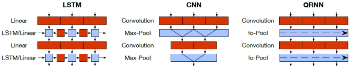
Figure 2.9 displays the computation structure of the QRNN in comparison with LSTM and CNN architectures. The red color implies convolutions and the blue color parameterless functions that operate in parallel along the channel/feature dimension. A continuous block means that those computations can proceed in parallel [29].

Figure 2.9: Computation structure of the QRNN (Original figure from [29])

2.3.3.2 Variants

Quasi recurrent neural network was the base for some other models in the field of the text analysis.

Encoder-Decoder

An extension of the QRNN model is the encoder-decoder model [29]. This archi-tecture uses a QRNN as encoder and a modified QRNN, enhanced with attention, as decoder. By feeding the last encoder hidden state (the output of the encoder’s pooling layer) into the decoder’s recurrent pooling layer would not allow the en-coder state to affect the gate or update values that are provided to the deen-coder’s pooling layer. This fact would substantially limit the representational power of the decoder. Instead, the output of each decoder QRNN layer’s convolution functions is supplemented at every timestep with the final encoder hidden state. The QRNN encoder–decoder architecture used for machine translation experiments.

Multi-fit

At Fast.ai, they presented an approach for exploiting QRNNs. Initially, Universal Language Model Fine tuning (ULMFiT) is a transfer learning method which can be used for NLP tasks [41]. ULMFit outperforms the state of the art on various text classification tasks (sentiment analysis, question classification, topic classification), reducing the error by 18-24% on the majority of datasets. Recently, in the paper [36], the authors proposed the Multi-lingual language model Fine-tuning (MultiFit)

(28)

2. Theory

for training and fine tuning language models efficiently.

The MultiFit model combines the ULMFit, with QRNNs and subword tokeniza-tion. The ULMFit model is based on a 3-layer AWD-LSTM (Averaged SGD Weight-Dropped LSTM) model, which is an approach that uses a DropConnect mask on the hidden to hidden weight matrices, in order to prevent overfitting across the recurrent connections [51]. The creators of the MultiFit replaced the LSTM with a QRNN to achieve a faster training. The MultiFit model evaluated on cross-lingal classifi-cation datasets and the researchers found that their model outperforms the models LASER, architecture for multilingual sentence representations in 93 languages which uses a BiLSTM encoder [26] and multi-lingual BERT, a language representation model based on the transformer encoder model [35]. Specifically, for the document classification task, MultiFit achieved the best accuracy in comparison with Laser and MultiBert over seven languages. Indicatively, for the Spanish language, Laser achieved an accuracy of 88.75, MultiBERT 95.15 and MultiFit 96.07.

2.3.4

Transformers

Transformers are machine learning models that use a combination of stacked en-coders and deen-coders which use the concept of attention [61]. This is implemented in the ’multi-head attention’ stage of the model. This gives the model the abil-ity to focus on positions in the environment of the token in consideration. It also gives the model multiple representation subspaces. As each of these attention heads are initialised randomly, each of the input embeddings is projected on to multiple representational subspaces. These models have the ability to understand word re-lationships very well due to the presence of hidden states at each stage of encoding and decoding along with the use of multi headed attention.

2.3.4.1 Model

A brief layout of the transformers model is show in Figure 2.10. The encoder blocks can be seen on the left and decoder blocks on the right. The input sequence is first embedded using a system called ELMo. ELMo is a contextual word embedding system that has been trained on a large multilingual data set so it embeds grouped words closely together. The embedded input sequence is first passed through the multi-head attention. This part of the model consists of a stacked attention layers that uses the query-key-value system to understand what embeddings to give more "attention" to for each word. Once these scores are obtained, they are passed through the feed forward section of the encoder to obtain the hidden state for that particular encoder. That hidden state is then passed over to the decoder which uses a similar system of multi headed attention to check for embedding relationships and to use a final sof tmax layer for an output probability distribution.

2.3.4.2 Variants

The transformer architecture based model, BERT, is an encoder only model that uses a combination of concepts such as Feature extraction, ELMo (Embeddings from Language models) and masked language modelling [35]. The first stage of

(29)

2. Theory

this model involves the multi-lingual embeddings of the words in the input text to obtain features. These features are then passed on to the stacked multi-layer en-coder (which are equipped with multi-head attention) architecture to understand and build feature relationships and dependencies. Once the combination of various types of features have been built, this data is then passed on to an output linear layer with asigmoid function to give out the probability distribution for each class. The embedder and encoder sections of the model have been pre-trained where as the final linear classification layers are added on according to the requirements of the classification. The transfer training can be done by either freezing the embed-der and encoembed-der sections while training the classifier weights or by fully retraining the classification weights for the entire model (including the embedder and stacked encoder sections).

Figure 2.10: Structure of a transformer (Original figure from [23])

2.4

Evaluation and Metrics

A classifier which has been employed for a multi label text classification task might predict all the expected labels, a subset of them, or none of the expected labels. Hence, those cases should be considered in order to evaluate the classifier. The met-rics for a multi label text classification problem are organized in two main categories which are example based and label based evaluation [59].

(30)

2. Theory

Example based evaluation

Consider a defined experiment with P positive instances and N negative instances for some condition. The four predicted outcomes can be classified into True Posi-tives (tp), False PosiPosi-tives (fp), True NegaPosi-tives (tn) and False NegaPosi-tives (fn) as the Table 2.1 explains.

Relevant Non relevant Retrieved true positives (tp) false positives (fp) Not retrieved false negatives (fn) true negatives (tn)

Table 2.1: Confusion matrix (Original table from [50])

The example based evaluation metrics that are being used are then defined as: • Recall: The percentage of predicted true labels to the total number of actual

true labels, Equation 2.1.

• Precision: The percentage of correctly predicted true labels to the total number of predicted true labels, Equation 2.2.

• F1-Measure: The harmonic mean of recall and precision, Equation 2.3. • Hamming loss: The hamming loss is the fraction of labels that are incorrectly

predicted [8], Equation 2.4.

Higher value of accuracy, precision, recall and F1- score, means better performance of the learning algorithm. The hamming loss metric, as its name declares, is a loss function so a lower value implies better performance.

Recall = tp tp+f n (2.1) P recision= tp tp+f p (2.2) F1 = 2P recision×Recall P recision+Recall (2.3) HammingLoss= 1 |N|.|L| i=1 X |N| j=1 X |L|

xor(yi,j, zi,j) (2.4)

where yi,j is the target, ji,j is the prediction, N is the number of classes and L the

number of the instances.

Label based evaluation

Label based measures evaluate each label separately and then averages over all labels. All the measures from the example based evaluation can be used for label evaluation.

• Micro averaged measures: Any of the example based evaluation metrics can be computed on individual class labels first and then averaged over all classes. • Macro averaged measures: Any of the example based evaluation metrics can

(31)

2. Theory

• Weighted average measures: Any of the example based evaluation metrics can be computed on individual class labels first and then averaged over all classes with their corresponding class weights. These class weights are given by the distribution of the test data.

2.5

Summary

The described models have been chosen as they are relevant to this particular prob-lem of this master’s thesis. A model which utilizes tf-idf vectorization and relies on support vector machines will be developed as a baseline model. Gated Recurrent Units with attention seems a safe approach for the specific problem. As the Convo-lutional Neural Network is based on the character level, the language of the input data will not be relevant in this case and the specific network sounds a promising model. Furthermore, a Quasi Recurrent Neural Network based model will be de-veloped since it enhances the performance. The Transformers model with the Bert multilingual encoder, negates the problem about having multilingual input data and therefore its performance will be evaluated on the given data set.

A major key of the email multi label classification task is the evaluation of the models. The precision aims to answer the question, what proportion of positive identifications was actually correct, while the recall tries to answer, what proportion of actual positives was identified correctly [3]. The F1 measure metric compromises between recall and precision so it is a good candidate. Macroaveraging metrics give equal weight to each class, whereas microaveraging metric give equal weight to each sample classification decision. Microaveraged metrics are a measure of effectiveness of the large classes in a test set. The effectiveness of the small classes can be represented better by the macroaveraged metrics [50]. Therefore the metrics that will be used for evaluating the results of each classifier will be precision, recall and F1 measure. The comparison of the performance among all models will be rely on the metrics weighted average F1, since the data set is unbalanced, and hamming loss.

(32)

(33)

3

Methods

A flowchart representing the steps that are being followed in this project is show in figure 3.1. The flowchart contains the SVM model, which acts as baseline model, as well as four deep learning models. The procedure starts by preprocessing and clearing the input data. After that, five different models (classifiers) will be trained on the data. The 90% of the data set has been used as training and validation data set, while the rest 10% has been used for testing. Then the trained models will be evaluated before delivering the results.

Figure 3.1: Pipeline flowchart

3.1

Preprocessing

The preprocessing of the input data is done in various stages. Initially, the obtained data set is grouped according to classes that have similar information and this brings the number of labels down from 107 to 14. The first of these stages then involves the removal of confidential information. Data such as names, numbers, web IDs, company names and mail ids were replaced with tags before the data was handed over. These tags have to be removed first. This is then followed by the removal of escape sequences, special characters, forwarded messages and other numbers. After this, greetings and brevity signatures (in Swedish and English) are removed. The obtained text is then trimmed to remove excess spaces. Next, the stop words are removed for both languages. This is done by creating a CSV file with the stop words that are to be considered and then searching for, and removing these words in each data point in the given data set.

The next step involves the stemming or lemmatization of the data. Both these procedures are done in a word by word fashion as they are language specific. Stem-ming is done by detecting the language of each word and applying the corresponding stemmer using the classSnowballStemmer [11] from the nltk[10] library. Lemma-tization is done by first detecting the language of each word using the langdetect

(34)

3. Methods

[17] library. The English words are then taken back to their lemma using the

W ordN etLemmatizer[46] from thenltklibrary. The Swedish words are lemmatized by comparing and substituting each word found to a CSV file consisting of words and their corresponding lemmas. The next stage of preprocessing is to remove all the proper nouns in the text. This is done using a combination of apostagger and a check to see if the words that are tagged as proper nouns are not actually words that are existent in the Swedish or English language lexicon (from the corresponding word lists).

Finally, the subject and the body of the email have been merged into one text sample. Usually, the subject of the email contains contextual information which enhances the label prediction.

3.2

Models

The output of the preprocessing and cleaning data procedure will be the input data set for the training models. One baseline model, SVM, and four deep learning mod-els have been employed for classifying the emails and comparing the results and the performance among them.

Support vector machines

A basic machine learning model has been built for the multi label text classifica-tion task. This model uses the tf-idf tokenizer in order to exploit the weight of the interesting and meaningful terms, which contribute to label prediction. Then, the model employs the OneVsRestClassifier [12], which fits one classifier per class. The decision function for the classifier has been set to LinearSVC as it is a fast approach [9].

Gated recurrent units with attention

The model is built using layers of stacked Gated Recurrent Units and self attention with alternating dropout layers in between. This is then followed by a linear layer with fourteen units, each for one class, and finally a sigmoid layer to give out the probability for each class. This model is then trained on the cleaned input data and tuned accordingly to improve performance. It is then evaluated on the test data based on the metrics and the results are noted.

Very deep convolutional neural networks

The very deep convolutional neural network (VDCNN) is a character based model. The alphabet consists of the English characters, which are common also in the Swedish alphabet, and the Swedish special characters like å, ä and ö. Each sample is converted in a vector where each character of the sample has been replaced by its index in the alphabet. The vectors are padded with zeros so that they have the same length. The network contains 9 convolutions layers and 3 pooling operations. The prediction part is handling by a k-max pooling function, which extracts the

k-highest activations from a sequence. The results of the k-max pooling function is the input to a three layer fully connected classifier with ReLU hidden units and sigmoid outputs. The very deep CNN model utilizes a Stochastic Gradient Descent

(35)

3. Methods

(SGD) optimizer with momentum [16]. The specific optimizer has been selected because it increased the efficiency for the specific combination of the model, data set and problem.

Quasi recurrent neural networks

The QRNN uses words as tokens and it is a really simple model. Specifically, it constists of a SpatialDropout1D, a QRNN and a Dense layer while the last acti-vation layer is a sigmoid actiacti-vation. The SpatialDropout1D layer [18] drops entire 1D feature maps instead of individual elements. The oprimizer for this network has been set to RMSprop, which implements the RMSprop algorithm [14].

Transformers

The transformers model is built using the pre-trained twelve encoder (BERT Base) stack and an additional dense layer and sigmoid activation function to obtain the probability distribution for the classes as an output. Initially the pre-trained weights of the model are frozen with only the final layer weights unfrozen and the model is trained on the training dataset. The model weights are then unfrozen entirely and the model is then trained on the cleaned and pre-processed training set. It is then evaluated on the test set and the results are noted.

The Table 3.1 presents an overview of some key components of the architecture of the deep learning models.

Model Token Last layer activation Optimizer

GRU byte-pair sigmoid SGD

Very deep CNN character sigmoid SGD

QRNN word sigmoid rmsprop

Transformers byte-pair sigmoid SGD

Table 3.1: Architecture overview of deep learning models

3.3

Evaluation

Once the training procedure has been completed the next step is to evaluate the classifier. After the training procedure each classifier predicts the output on the test data set by producing the classification report. The classification report is a text report which shows the main classification metrics like precision, recall and so on for each class. This is a mere task which is performed by calling the classification report function from sklearn [4]. In addition, thehamming loss for each classifier is computing by using the homonym function from sklearn [8].

(36)

(37)

4

Results

This chapter includes a detailed analysis of the data set as well as a comprehensive presentation of the results that have been delivered by the developed models.

4.1

Dataset

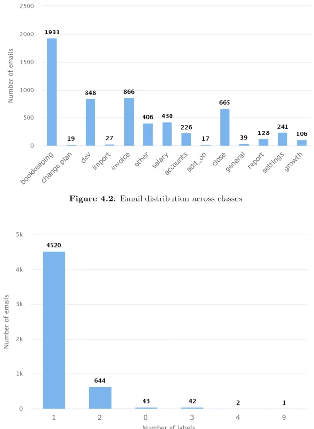
The results from the exploratory data analysis have been shown in figures 4.1 , 4.2 and 4.3. The training data set consists of a total of 5272 emails. Figure 4.1 gives information about the number of characters per input data point as a histogram. According to the histogram the average length of the emails is approximately 370 characters for the majority of the emails. The Figure 4.2 gives an idea about the classwise distribution of data across the input data set. The majority of the emails belongs to the class bookkepping, while the classes invoice, dev and close are fol-lowing. Latest Figure 4.3 displays the number of emails which have multiple labels. The vast majority of the emails has only one label and a small portion has two labels.

(38)

4. Results

Figure 4.2: Email distribution across classes

Figure 4.3: Emails with multiple classes

Lingual distribution of emails

(39)

4. Results

• Swedish and English: These emails make up a majority of the data set and they contain both Swedish and English words in the same mail. There are 4973 emails in this category.

• Swedish: These emails consist of only Swedish words. There are 202 emails in this category.

• English: These mails consist of only English words. There are 96 emails in this category.

Description of the content of the classes

A brief description of the contents of emails in each of the classes is shown at the table 4.1. Moreover, the Appendix A presents same email samples that belong to the below classes.

Class Description

bookkeeping emails from customers that have queries or doubts about the bookkeeping services that are offered by the company

change plan emails that are from customers that request a change in subscription plans and renewals of services

dev

queries or feedback from customers about the actual functionality or usage of the services and doubts about factors like login

information and mistakes while reporting or updating information import

emails that have customer queries about importing invoices and the settings relating to the same. These emails also deal with questions about errors while importing e-invoices

invoice emails from this class deal with customer queries and questions about invoices in general

other emails that are received by the company that cannot be categorised into any of the classes belong to this class salary queries from companies and organizations that are based on

salaries of the employees and their relevant tax benefits accounts

emails in this category deal with customer feedback and suggestions about the functioning of the accounting systems by the company

add on emails that are relevant to the addition of services which are related to account and billing

close emails about the closure and termination of particular services that are offered by the company

general generic queries about accounting and services.

report emails deal with the queries about balance reports and verification settings emails in this class deal with the queries about settings of the

accounts of customers growth

emails in the growth class deals with problems and shortcomings with the support that has been

reported as feedback from customers

(40)

4. Results

4.2

Model Performance

The next sections present the results, by including the classification report and hamming loss, as they have been delivered by each classifier.

4.2.1

Support vector machines

The SVM model delivered a hamming loss equals to 0.0077. The table 4.2 presents the classification report for this baseline model. As it can be concluded by the table, the efficiency of this model is high. The OneVsRestClassifier which has been used for this model employs one classifier per class. Since each class is represented by one and one classifier only, it is possible for each classifier to gain knowledge and draw the contextual window for each particular class.

Class Precision Recall F1-score Support bookkeeping 1.00 1.00 1.00 46 change plan 1.00 1.00 1.00 19 dev 0.97 0.97 0.97 36 import 1.00 0.95 0.98 22 invoice 1.00 0.90 0.95 30 other 1.00 0.97 0.99 37 salary 1.00 0.96 0.98 23 accounts 1.00 0.92 0.96 25 add_on 1.00 0.88 0.94 17 close 1.00 0.82 0.90 39 general 1.00 1.00 1.00 23 report 1.00 0.91 0.95 23 settings 1.00 0.83 0.90 23 growth 1.00 0.83 0.91 24 micro avg 1.00 0.93 0.96 387 macro avg 1.00 0.93 0.96 387 weighted avg 1.00 0.93 0.96 387 samples avg 0.97 0.94 0.95 387

Table 4.2: SVM classification report

4.2.2

Gated Recurrent Units with attention

The Table 4.3 depicts the performance of the Gated Recurrent Unit with attention model. The evaluation has an overall hamming loss of 0.0447 for this model. From figure 4.4, it can be seen that the GRU model overfits the data. This can be attributed to a number of reasons ranging from the distribution of the data across the classes and the nature of the data itself. It can also be seen that despite using class weights to compensate for the unbalanced distribution, the classes with a higher number of samples in the train set (such as bookkeeping, dev and other)

(41)

4. Results

have much better performance than the other classes. It can also be noted that the rather negligible difference between the micro averaged and macro averaged precision scores shows that the major difference in performance due to class imbalances does not affects recall a lot more than it affects precision. The difference between the micro and macro averaged recall is a lot higher, hence, showing that the model more confidently classifies emails that belong to the classes with a larger population.

(42)

4. Results

Figure 4.4: GRU training and validation loss

4.2.3

Very deep CNN

The training of the very deep CNN model ended with a hamming loss equals to 0.0235 and the Table 4.4 illustrates the classification report of this model. Overall the specific model achieved a good performance. Excluding the classes dev, invoice, accounts and growth the rest classes hold a greater or equal precision than recall. This character based model managed to find and learn the representations for the specific problem of the samples, which are containing two languages at the same time. The figure 4.5 displays the training and validation loss function through the 40 epochs which has been used for training this model. In the end of the training the validation loss is almost 0 but the validation loss is 0.6 which means that the model tends to overfit.

This model relies on the research work of the Facebook AI [34] and the contrib-utors show that the performance of this model increases with the depth. They used up to 29 convolutional layers and they reported improvements over the state of the art on several public text classification tasks on large scale data sets. The length of the samples of their data sets varies among them and there was a case where the data set included samples with an average text length of 764 characters. However, for the multi label text classification task on bilingual texts, increasing the depth and using 17 or 29 convolutions layers downgraded significantly the performance of the very deep model. The average text length of this master’s thesis data set is around 370 characters which is not far away of the shortest text length that they used. The big difference is the size of the data set. The smallest training data set that they used, consists of 120 thousands examples, while the training data set of this master’s thesis is only 5 thousands. However, despite the small size of the data

(43)

4. Results

set the very deep CNN model delivered remarkable results.

Table 4.4: Very deep CNN classification report

(44)

4. Results

4.2.4

Quasi Recurrent Neural Network

The QRNN model holds a hamming loss of 0.0375 and the Table 4.5 depicts the classification report for the QRNN model. In the QRNN model the recall is greater than the precision for 9 out of 14 classes. Excluding the classes change plan, dev, import, other and add_on, the rest of the classes hold greater or equal recall rather than precision. The Figure 4.6 illustrates the training and validation loss through 40 epochs. In the end of the training the training loss is around 0.05 while the validation loss is close to 0.6, which means that the QRNN model seems to overfit.

(45)

4. Results

Figure 4.6: QRNN training and validation loss

4.2.5

Transformers

The Table 4.6 depicts the performance of the BERT Transformers model using transfer learning. The evaluation has an overall hamming loss of 0.0461 for this model. From figure 4.7 it can be seen that the model grossly overfits the dataset. A primary issue is the fact that the pre-trained section of the BERT 12 stack encoder model is fixed in size, which in this case makes the model overfit the input data. A large difference between the micro and macro average in the precision metric also tells us that the BERT model is the most affected by the class imbalances. It can also be seen that the precision is lesser than the recall in the micro,weighted and macro fields, which is in line with the model overfitting. This means that since the model has fit the training data very well it is "falsely confident" about the predictions that are made in the evaluation phase and hence the model tends to make predictions that may not be right, confidently, thereby causing this behaviour.

(46)

4. Results

Table 4.6: Transformers classification report

(47)

5

Conclusion

This chapter concludes this master’s thesis by discussing the methods and results as well as giving ideas for future work.

5.1

Discussion

Five different models have been developed for studying the multi label email classifi-cation task with the special case of bilingual texts, English and Swedish, at the same time, having to deal also with a size limited and unbalanced data set. One simple model, SVM, and four deep learning models with major differences in their archi-tecture have been employed in order to examine their behaviour and performance in this particular problem. This section provides a discussion for the results that have been delivered from the models, as well as the contribution of the stemming and lemmatization in the final results.

5.1.1

Results comparison among the models

The Table 5.1 presents a summary of the weighted average F1 score and hamming loss among the developed models. The SVM outperforms the four deep learning models. The best deep model is the very deep CNN with a weighted average F1 score of 0.89 against the SVM with 0.96 score. The second best deep learning model is the QRNN with 0.80 weighted avg F1 score.

SVM GRU Very deep CNN QRNN Transformers Weighted avg F1 0.96 0.67 0.89 0.80 0.53

Hamming loss 0.0077 0.0447 0.0235 0.0375 0.0461

Table 5.1: Metrics comparison among the models

From the performance tables in chapter 4, it can clearly be seen that the SVM model gives the best results according to the chosen metrics. The main reason is that the SVM uses the OneVsRestClassifier which employs one classifier per class. In this way each classifier is able to learn about word relationships and class associations really good. A known reason which downgrades the performance of the deep learning models involves the size of the data set and the distribution of emails in it. The specific data set is on the smaller side and with an extremely unbalanced distribution. A comparison between the deep learning models shows that their performance varies a lot among them and their architecture causes a different behaviour. In the

(48)

5. Conclusion

case of the GRU model, the precision is higher ( 91%) but the lower recall brings the F1-measure down. The very deep CNN delivered the best results among the deep learning models, giving a higher precision. A major factor for it’s performance is that it uses characters as tokens which proved a real good approach for the specific case. This character based model was able to find good representations, handle the both languages simultaneously and learn sufficiently the relationships between the samples and classes. The QRNN model delivered the second best results among the deep learning models. The QRNN model is using words as tokens and it is a simple model in contrast with the very deep CNN, which delivered the best results, among the deep learning models. Those two models, very deep CNN and QRNN, are greatly differing in terms of architecture perspective, but both of them delivered good results. The CNN employs a convolutional layer while the QRNN utilizes a dense layer. The major difference between those two layers is that the dense layer learns global patterns while the convolutional layer learns local patterns [32] and this is the reason that the CNN model delivered better results than the QRNN model. The performance of the BERT model is the lowest, with respect to F1-measure, precision and recall. This is due to the fact that the byte pair word embedding combined with the relatively large size of the pre-trained section means that the model overfits the data drastically. It is also the most affected by the class distribution of the data set. In this multi label email classification, the precision represents how many of the predicted labels actually belong to that sample, while the recall represents how many relevant labels from that sample were found. The GRU and the very deep CNN delivered greater or equal precision rather than recall for the most of the classes. Particularly, the precision was higher for the 12 out of 14 classes for the GRU and for the CNN was for the 10 of the 14 classes. That means that the GRU and very deep CNN models were able to predict a big proportion of the positive identifications correctly while they missed some relevant labels. In contrast with the GRU and the very deep CNN, the QRNN model delivered greater or equal recall rather than precision for 9 out of 14 classes. Therefore, the QRNN model found a big proportion of the relevant labels for the samples. For the Bert model the number of classes with higher recall is almost equal to the number of the classes which present higher precision and therefore the Bert model doesn’t seem to change drastically the precision and the recall.

Additionally, Chapter 4 shows that the deep learning models overfit during the training, which means that the models learn more than enough information of the training data and so they are not able to make as good predictions on the new data as they delivered on the training data. Preventing overfitting can be done by 1) reducing the network’s size (capacity), 2) adding dropout and 3) getting more training data [32]. Reducing the network’s size is referred to decreasing the number of the layers. GRU and QRNN models are simple models with only a few number of layers. The CNN is a deep network, however it performs well on the testing data set, therefore the chosen capacity of the network doesn’t impair it’s performance. On the other hand the Bert model is a massively huge model, which might explains why it overfits. By adding a droupout layer in the networks will result in mitigating the noise of the output values, so the network will memorize only the significant patterns which contribute to the label prediction. All of the deep learning models

(49)

5. Conclusion

include at least one dropout layer. Therefore, enriching the training data set would prevent the overfitting.

5.1.2

Stemming vs Lemmatization

While using stemming instead of lemmatization as the method of linguistic mor-phology for the data set, certain differences were noticed in the performance of the models. In terms of weighted average F1 score it noticed that its value was down-graded by 8% for the SVM model, 7% for the CNN and 26% for the QRNN. In the case of BERT and the GRU models, the weighted average f1 score dropped by about 9% on average. One of the reasons for this is the fact that particular classes had a larger population of words such as "general", "organization" and "led", which were wrongly truncated to words that now did not make any sense. This meant that the model was not able to extract the right features from these pieces of text and caused a drop in performance while using a stemmer. To add to this, the QRNN (which has the biggest drop) is a model that uses word embeddings combined with a model that is contextually trying to understand information. This means that the stemmer affecting certain words and putting them out of context has a really large impact on the performance of this model in particular. To an extent, this impact can be seen on the GRU and BERT models as well, as they use sub-word embeddings.

5.2

Future work

In terms of future work there are some attractive points which are need further exploration. As it has been already mentioned MultiFit is a multilingual language model, which is currently available in seven different languages, Swedish language is excluded. It employs a QRNN which enhances the performance and according to the creators of the model, the MultiFit performs well on small data sets which contain only 1000 examples and outperforms Bert. Therefore the fact that the specific model outperforms other models even if it has been trained on small data sets, seems promising for the problem of this master’s thesis and it would be interesting to study how it performs on this bilingual small data set.

Another experiment with the specific data set and the chosen models it would be the case of enriching the data set before the training procedure. Enriching the initial data set, which is called data augmentation, by an arbitrary way it would result in overfitting due to the extra noise in the data. That’s way another approach like semantic enrichment would be interesting and it might improve the performance of the deep learning models.

5.3

Conclusion

From the experiments and results that have been obtained after evaluating the pipelines that have been built, the following points can be concluded for the specific problem of this master’s thesis: multi label text classification on short text, emails, with two languages, English and Swedish, at the same time and having a size limited

(50)

5. Conclusion

and unbalance data set.

Simple model performs better. The simple SVM model performs better than any of the other deep learning models that were evaluated.

Character based deep learning model performs better. The very deep char-acter based model delivered the best results among the deep learning models, with-out a big deviation from the SVM model. In this particular case with Swedish and English input text, the character level encoding performs a lot better than the byte-pair encoding. This could be due to the relatively common nature of the characters present in both languages, in the same data points.

Depth doesn’t improve performance. The contributors of the paper [34] con-cludes that the depth improves the performance of the very deep CNN. However in this particular case of the size limited and unbalanced data set the increment of the depth impaired the performance. The major difference between their experiments and those of this master’s thesis is the size of the data set. They were working with at least 120 thousands of examples for the training data set against the 5 thousands exam

Text analysis for email multi label classification