Causal Inference with Covariate Balance Optimization

(1)

Causal Inference with Covariate

Balance Optimization

by

Yuying Xie

A thesis

presented to the University of Waterloo in fulfillment of the

thesis requirement for the degree of Doctor of Philosophy

in Statistics

Waterloo, Ontario, Canada, 2018

c

(2)

Examining Committee Membership

The following served on the Examining Committee for this thesis. The decision of the Examining Committee is by majority vote.

External Examiner: Robert Platt

Professor, McGill University

Supervisor(s): Yeying Zhu

Assistant Professor Cecilia Cotton Associate Professor

Internal Member: Michael Wallace

Assistant Professor

Internal Member: Changbao Wu

Professor

Internal-External Member: Pierre Chauss´e

(3)

I hereby declare that I am the sole author of this thesis. This is a true copy of the thesis, including any required final revisions, as accepted by my examiners.

(4)

Abstract

Causal inference is a popular problem in biostatistics, economics, and health science studies. The goal of this thesis is to develop new methods for the estimation of causal effects using propensity scores or inverse probability weights where weights are chosen in such a way to achieve balance in covariates across the treatment groups.

In Chapter1, we introduce Neyman-Rubin Causal framework and causal inference with

propensity scores. The importance of covariate balancing in causal inference is furthered discussed in this chapter. Besides, some general definitions and notations for causal in-ference are provided with many other popular propensity score approaches or weighting

techniques in Chapter 2.

In Chapter3, we describe a new model averaging approach to propensity score

estima-tion in which parametric and nonparametric estimates are combined to achieve covariate balance. Simulation studies are conducted across different scenarios varying in the degree of interactions and nonlinearity in the treatment model. The results show that the proposed method produces less bias and smaller standard errors than existing approaches. They also show that a model averaging approach with the objective of minimizing the average Kolmogorov-Smirnov statistic leads to the best performance. The proposed approach is applied to a real data set in evaluating the causal effect of formula or mixed feeding versus exclusive breastfeeding in the first month of life on a child’s BMI Z-score at age 4. The data analysis shows that formula or mixed feeding is more likely to lead to obesity at age 4, compared to exclusive breastfeeding.

In Chapter 4, we propose using kernel distance to measure balance across different

treatment groups and propose a new propensity score estimator by setting the kernel distance to be zero. Compared to other balance measures, such as absolute standardized mean difference (ASMD) and Kolmogorov Smirnov (KS) statistic, kernel distance is one of the best bias indicators in estimating the causal effect. That is, the balance metric based on kernel distance is shown to have the strongest correlation with the absolute bias in estimating the causal effect, compared to several commonly used balance metrics. The kernel distance constraints are solved by generalized method of moments. Simulation studies are conducted across different scenarios varying in the degree of nonlinearity in both

(5)

the propensity score model and outcome model. The proposed approach produces smaller mean squared error in estimating causal treatment effects than many existing approaches including the well-known covariate balance propensity score (CBPS) approach when the propensity score model is misspecified. An application to data from the International Tobacco Control (ITC) policy evaluation project is provided.

Often interest lies in the estimation of quantiles other than the average causal effect. Other quantities such as quantiles or the quantile treatment effect may be of interest.

In Chapter 5, we propose a multiply robust method for estimating marginal quantiles

of potential outcomes by achieving mean balance in (1) the propensity score, and (2) the conditional distributions of potential outcomes. An empirical likelihood or entropy measure can be utilized instead of using inverse probability weighting. Simulation studies are conducted across different scenarios of correctness in both the propensity score models and outcome models. Our estimator is consistent if any of the models are correctly specified.

(6)

Acknowledgements

First and foremost I want to offer my sincerest gratitude to my supervisors, Dr. Yeying Zhu and Dr. Cecilia Cotton, who have supported me throughout this thesis with their patience, extensive knowledge and experience. They always support and encourage me to overcome any obstacles I have been facing through my PhD studies. Without their advice and insights, it would be impossible for me to complete this thesis. They became more of mentors and friends, than supervisors, which I truly appreciate. One simply could not wish for a better or friendlier supervisor, I am very grateful to have them as my supervisors.

I would also like to thank the rest of my thesis examining committee: Dr. Robert Platt,

Dr. Pierre Chauss´e and Dr. Changbao Wu, and Dr. Michael Wallace for taking their time

to read my thesis, and for all the thoughtful and invaluable comments they give.

In addition, I am grateful to the department faculty and staff, for the knowledge I have learned and all the help and support I have received.

Many thanks go to my dear friends, who have supported me all the way. I am grateful for their friendship, encouragement, and the wonderful times we spent together.

Last but not the least, I would like to thank my parents and brother for their uncondi-tional love. My special thanks go to Xinjie, who has always been encouraging me to follow my dreams.

(7)

(8)

4.6.1 Proof of Theorem 4.6.1 . . . 66 4.6.2 Proof of Lemma 4.6.2 . . . 67 4.6.3 Proof of Theorem 4.2.1 . . . 68 4.6.4 Proof of Theorem 4.2.2 . . . 69 4.6.5 Proof of Lemma 4.6.3 . . . 70 4.6.6 Proof of Lemmas 4.6.4 - 4.6.7 . . . 71 4.6.7 Proof of Theorem 4.2.3 . . . 76 4.6.8 Proof of Theorem 4.2.4 . . . 77

(10)

5 Multiple Robust Estimation of Causal Quantile Treatment Effects 78

5.1 Framework for Quantile Treatment Effect . . . 79

5.2 Proposed Approach . . . 80

5.2.1 Entropy Measure Approach . . . 83

5.3 Theoretical Properties . . . 84

5.3.1 Consistency of the Quantile Estimator . . . 84

5.3.2 Asymptotic Normality of the Quantile Estimator . . . 85

5.4 Simulation Studies . . . 86

5.4.1 Simulation Setup . . . 86

5.4.2 Simulation Results . . . 88

5.5 Application . . . 89

5.6 Conclusion . . . 95

5.7 Theorems and Proofs . . . 97

5.7.1 Proof of Theorem 5.3.1 . . . 97

5.7.2 Proof of Theorem 5.3.2 . . . 100

5.7.3 Proof of Theorem 5.3.3 . . . 101

5.7.4 Proof of Theorem 5.3.4 . . . 107

6 Discussion and Future work 109 6.1 Discussion . . . 109

6.2 Future work . . . 111

References 113

(11)

A More Simulation Results 125

A.1 Appendix for Chapter 3 . . . 125

A.1.1 More Simulation Results for Chapter 3 . . . 125

A.2 Appendix for Chapter 5 . . . 128

(12)

List of Tables

3.1 Performance of Measures by Propensity Score Models in 1000 Simulated Data Sets with n= 1000 (Estimation of ACE). . . 27

3.2 Analysis of Breastfeeding Data with Continuous Outcome (Estimation of ACE, Samples=500) . . . 34

3.3 Analysis of Breastfeeding Data with Binary Outcome (Estimation of RR, Samples=500) . . . 35

4.1 Coefficients for Propensity Score Models . . . 50

4.2 Coefficients for Outcome Models . . . 51

4.3 Performance for Estimation of ACE by Propensity Score Approaches (n = 1500) . . . 53

4.4 Performance for Estimation of ACE by Propensity Score Approaches (n = 1000) . . . 54

4.5 Performance for Estimation of ACE by Propensity Score Approaches (n= 500) 55

4.6 Bias for KDPS with Different σ2 _{. . . .} ₅₆

4.7 Standard Error for KDPS with Different σ2 _{. . . .} ₅₆

4.8 Mean Squared Error for KDPS with Different σ2 _{. . . .} ₅₆

4.9 Simulation Results for Estimation of ACE, Absolute Bias between ASE and

(13)

4.10 Summary for the Significance of Each Covariate in the ITC wave=8 Canada Dataset from Univariate Regression Models. . . 59

4.11 Average Causal Effect between Observations Who Participated through Web Survey versus Telephone Survey . . . 61

5.1 Scenario 1A: Simulation Results of QTE and DR Estimators with 50th Per-centile (n = 1000) . . . 90

5.2 Scenario 2A: Simulation Results of QTE and DR Estimators with 50th Per-centile (n = 1000) . . . 90

5.3 Scenario 1B: Simulation Results of QTE and DR Estimators with 50th Per-centile (n = 1000) . . . 91

5.4 Scenario 2B: Simulation Results of QTE and DR Estimators with 50th Per-centile (n = 1000) . . . 91

5.5 Scenario 3C: Simulation Results of QTE and DR Estimators with 50th Per-centile (n = 1000) . . . 92

5.6 Quantile Treatment Effect Estimate for 50th Percentile with Birthweight Data 95

A.1 Performance of Measures by Propensity Score Models in 1000 Simulated Data Sets with n= 100 (Estimation of ACE). . . 126

A.2 Performance of Measures by Propensity Score Models in 1000 Simulated Data Sets with n= 5000 (Estimation of ACE) . . . 127

A.3 Scenario 1A: Simulation Results of QTE and DR Estimators with 25th Per-centile (n = 1000) . . . 128

A.5 Scenario 1B: Simulation Results of QTE and DR Estimators with 25th Per-centile (n = 1000) . . . 129

(14)

A.19 Scenario 3C: Simulation Results of QTE and DR Estimators with 50th Per-centile (n = 5000) . . . 137

(15)

A.24 Scenario 3C: Simulation Results of QTE and DR Estimators with 50th Per-centile (n = 200) . . . 140

(16)

List of Figures

1.1 Causal Diagram with Confounders . . . 2

3.1 Boxplots of ACE Estimates across All Simulation Scenarios (n = 1000 units, 1000 replications) . . . 28

3.2 Boxplots of Estimated λ for the Four Model Averaging Methods across All Simulation Scenarios (n = 1000 units, 1000 replications) . . . 30

3.3 Distribution of Inverse Probability Weights for 10 Random Datasets of size

n = 1000. . . 31

3.4 Plots of Weighted ASMD versus Unweighted ASMD (Red Line for Cut-off Value 0.1, Black Line for Cut-off Value 0.2). . . 36

3.5 Plots of Weighted KS Statistics versus Unweighted KS Statistics (Red Line for Cut-off Value 0.1, Black Line for Cut-off Value 0.2) . . . 37

4.1 Causal Diagram among Variables in the Simulation Setup. . . 48

4.2 Empirical Cumulative Distribution Functions for Treatment and Control Groups across Covariates under Simulation Scenario 1A . . . 49

4.3 Boxplots of Weights by Propensity Score Approaches in ITC Data Analysis 62

4.4 ASMD Values for Each Covariate under KDPS and CKDPS before and after Balancing in ITC Data Analysis . . . 63

(17)

5.1 Infant Birthweight Distributions for Smoking and Non-smoking Mother Groups

. . . 93

(18)

Chapter 1

Introduction

1.1

Neyman-Rubin Causal Framework

Causal inference is pervasive in many fields. In health research, researchers are interested in questions such as “What causes the disease?” or “Will aspirin reduce headaches?” In eco-nomics studies, researchers may ask “What are the factors driving increased gas prices?” In randomized trials, researchers measure the magnitude of causal effects by comparing the outcome when an action is applied with the outcome when no action is applied. The action is commonly known as a treatment, exposure or intervention. Confounders are vari-ables that affect both the treatment assignment and the outcome. In randomized studies, treatments are randomly assigned to subjects. Random allocation ensures that there are

no measured or unmeasured baseline characteristics as confounders. Figure 1.1 shows the

causal diagram for a nonrandomized study with treatment assignment T, confounders X,

and outcome variable Y. For a randomized study, there is no edge from X toT.

Estimat-ing a causal effect in randomized studies is straightforward because any covariates that might influence the outcome can be assumed to have the same distribution across different treatment groups. Therefore, any difference in the outcome variable across the groups can be attributed to the different treatments.

There is increasing interest in observational studies to draw causal inference when the treatment assignment is not random. In non-randomized studies, there may be confounders

(19)

T Y

X

Figure 1.1: Causal Diagram with Confounders

that impact both the outcome and the treatment assignment. Baseline characteristics of treated subjects can differ greatly from the characteristics of untreated subjects. Ignoring these confounders may lead to biased estimation of the causal effects.

In this thesis, we work within the potential outcomes framework, also known as the

Neyman-Rubin Causal Model, for estimating causal effects (Rubin,1974;Splawa-Neyman

et al., 1990; Holland et al., 1985; Imbens and Rubin, 2015). A potential outcome is the

hypothetical value of the outcome variable for a subject under a specific treatment (Rubin,

2008). If we use i to index individuals and Yi for the outcome of the ith subject, each

individual has a pair of potential outcomes under the binary treatment setting. We use

Yi(1) to denote the potential outcome under treatment, while Yi(0) denotes the potential

outcome under the control.The control here refers to no treatment assignment throughout

the thesis. The individual causal effect can be defined as Yi(1) −Yi(0). Estimation of

the individual causal effect is not practical since we can never observe both {Yi(1), Yi(0)}

simultaneously. If the treatment is applied to subject i, Yi(1) is observed and Yi(0) is

sometimes called the counterfactual outcome. On the other hand, if the treatment is not

applied to subject i, Yi(1) will be the counterfactual outcome and Yi(0) will be observed.

The causal quantity we are interested in estimating is often the average causal effect, which is defined as the difference in the potential outcomes within the same subject averaged

over a given population: E{Y(1) −Y(0)}. The causal risk ratio (E{Y(1)}/E{Y(0)} =

P{Y(1) = 1}/P{Y(0) = 1}) is also an interesting quantity when we want to study the

incident proportion ratio between treatment and control groups.

Standard assumptions are essential under the Neyman-Rubin Causal Model to obtain

consistent causal effect in observational studies (Rosenbaum and Rubin, 1983; Cole and

(20)

• Consistency: A subject with an assigned treatment equal tothas observed outcome

Y equal to its potential outcome Y(t): Yi =Ti×Yi(1) + (1−Ti)×Yi(0).

• Strongly Ignorable Treatment Assignment: The treatment T assigned is inde-pendent of the counterfactual outcomes given the observed characteristics:

{Yi(1), Yi(0)} |= Ti|Xi.

• Stable Unit Treatment Value Assumption (SUTVA): Each subject’s potential outcomes should be unaffected by the actual treatment assignment of another subject.

• Positivity: 0< P(Ti = 1|Xi =x)<1.

The consistency assumption can be problematic when there are different versions of

treatment (Hernan and Vander Weele, 2011). For example, we want to study the average

effect between the heart transplant (treatment) and medical therapy (control) on patient’s 5 year mortality. The doctor may conduct the heart transplant in different pre-operative procedures. The average effect of heart transplant in a study where the doctors used a traditional pre-operative procedure may differ from that in another study where doctors tried a novel pre-operative procedure. The treatment is not well defined in this case.

The strongly ignorable treatment assignment assumption is also known as the no un-measured confounders assumption. It implies that conditional on baseline characteristics the treatment assignment is independent of the set of potential outcomes. If there is no

unmeasured confounders, one can still obtain unbiased estimates of causal effects (Robins

et al., 2000). The no unmeasured confounders assumption is not testable since Yi(0) is

not observed if treatment is assigned or Yi(1) is not observed if no treatment is assigned.

However, assessing the assumption is feasible (Imbens and Rubin,2015).

The SUTVA excludes the possibilities of units interfering with each other and multiple versions of a treatment but there are circumstances in which it is not credible. For example, it may be violated in a family study about some infectious diseases such as flu. If one family member receives a vaccine, it may affect the others’ change of getting flu.

The positivity assumption implies that each subject has a non-zero probability of re-ceiving either treatment or control. If a particular subpopulation has zero probability of

(21)

being assigned to the treatment, the estimation of causal effects will be based on

extrapo-lation and we may have to exclude such subpopuextrapo-lation from analysis (Imbens and Rubin,

2015).

1.2

Causal Inference with Propensity Scores

The propensity score is defined as the conditional probability of assignment to the

treat-ment group given the observed covariates (Rosenbaum and Rubin, 1983): e(x) = P(T =

1|X = x). Rosenbaum and Rubin (1983) also showed that, under the strongly ignorable treatment assignment assumption,

{Yi(1), Yi(0)} |= Ti|ei(X)

which means, given e(X), the distributions of potential outcomes are independent of the

treatment assignment. It plays an important role in estimating the causal effect in

obser-vational studies (Rosenbaum and Rubin,1983).

There are many approaches to estimate the average causal effect using propensity scores,

such as inverse probability weighting (IPW; Hirano and Imbens (2001)), stratification

(Rosenbaum and Rubin,1983), and matching (Cochran and Rubin,1973;Rubin,1973a,b). Causal inference based on propensity scores is usually a two step procedure. First the propensity score is estimated (for example using logistic regression). Then the causal effect is estimated by weighting the outcome using the inverse of the estimated propensity score for each subject or matching control subjects to treated subjects based on the similarity of the estimated propensity scores. These methods have been shown to be effective in

estimating the average causal effect (Hirano and Imbens, 2001; Stuart, 2010).

Logistic regression has frequently been used in observational studies to estimate the propensity scores for binary treatment. Traditional logistic regression is still found to be a good choice when the propensity score model is not heavily misspecified. Alternatively,

Lee et al. (2010) suggest using classification and regression trees (CART) (Breiman et al.,

1984), prune CART, and ensemble methods such as: bagged CART (Breiman, 1996),

(22)

2004) for propensity score estimation. All the above mentioned approaches are built on de-cision trees. Among these, GBM and random forest showed improvement over traditional parametric methods in terms of absolute bias, coverage rate, and reduction in standard

error (Lee et al., 2010). A random forest is a collection of decision trees based on

boot-strapped samples of the original data. For each split of the tree, a random subset of the

predictors is chosen and the best split is found among the chosen predictors (Friedman

et al., 2001). GBM (Friedman et al., 2001) is an iterative tree method that fits a tree model using residuals from the previous tree. Therefore, the trees are grown sequentially but not independently such as random forest.

Despite the popularity of IPW, Kang and Schafer (2007) found that the estimators

based on IPW are sensitive to the misspecification of the propensity score model. Many

double robust estimators (Robins et al.,1994,1995;Rotnitzky et al.,1998;Qin et al.,2008;

Tan, 2010; Fan et al., 2016) have been proposed by modelling the treatment assignment mechanism and the relationship between covariates and outcome to improve the efficiency. These methods are robust to the misspecification of one of the treatment or outcome models.

1.3

Covariate Balancing

Covariate balance means that the distributions of measured covariates for observations in

the treatment group and control group are similar to each other (Harder et al.,2010). Rubin

(2007) advocated mimicking randomized experiments since randomization is considered the

gold standard in estimating the average causal effect. It means analysis in observational studies can be modified to derive an estimator you would have derived when you run a randomized control trial. The baseline characteristics of observational studies are used to adjust the studies such that the subgroups of treatment and control units are similar to each other. Randomized design is usually infeasible due to many reasons including but not limited to time limit, ethical concerns, and massive expenses. However, this can be

accomplished by propensity score approaches, matching methods (Stuart,2010;Iacus et al.,

2012) or weighting based covariate balancing methods (Qin and Zhang,2007;Hainmueller,

(23)

Hence, achieving balance in covariates across treatment groups is one of the most important targets for propensity score based approaches to achieve the similarity of subgroups. By achieving balance in covariates, the bias in estimating the average causal effect can be

reduced (Harder et al., 2010). Mean balance is defined as the equivalence of the means of

the potential outcomes between the treatment and control groups (Hazlett, 2015). Under

strongly ignorable treatment assignment, Hazlett (2015) showed that if the mean balance

on a linear outcome model is achieved by weighting, an unbiased estimator of the average causal effect on the treated can be obtained. In this section, we give a brief introduction to the literature specifically focusing on covariate balancing.

Recently, several propensity score modelling approaches have been proposed which tar-get achieving balance in the covariates. For example, the GBM approach estimates the

propensity score through generalized boosted regression (McCaffrey et al.,2004). The

num-ber of iterations in GBM is determined by minimizing average standardized absolute mean difference such that the covariate balance is optimized. The covariate balancing propensity score method (CBPS) was introduced to model the treatment assignment using a logistic

model while simultaneously optimizing the covariate balance (Imai and Ratkovic, 2014).

The CBPS method estimates the parameters of the propensity score model by solving es-timating equations implied by the covariate balancing property while still incorporating

the standard logistic regression estimation procedure (Imai and Ratkovic, 2014). This

es-timation is conducted using generalized method of moments (GMM) (Hansen, 1982) or

empirical likelihood (Owen, 2001). The CBPS method optimizes the balance of

covari-ates between treatment and control groups. The advantage of CBPS is that it reduces

the effect of potential misspecification of a parametric propensity score model (Imai and

Ratkovic, 2014). Fan et al. (2016) discussed the theoretical properties, optimal choice of covariate balancing function for CBPS methodology and proposed a double robust and efficient improved-CBPS (iCBPS) methodology.

In addition to the commonly used matching and inverse propensity score weighting

ap-proaches in observational studies, entropy balancing was proposed byHainmueller(2012).

The entropy measure used in entropy balancing method is the measure of divergence from one distribution to another distribution. It differs from other preprocessing approaches by directly focusing on the goal of achieving covariate balance, which can help to reduce model

(24)

dependence while retaining valuable information. The entropy balancing method relies on a maximum entropy reweighting scheme that directly incorporates covariate balance into the weight function. The reweighting scheme includes a large set of balance constraints so that the covariate distributions in the treatment and control groups will match exactly on all pre-specified moments. The entropy balancing method is shown to be double robust when either the logistic propensity score model or the outcome model is linear in some

functions of covariates which is also used for balancing constraints. Hazlett (2015) also

proposed a kernel balancing method to find the weight vector such that the mean balancing on the kernel matrix is satisfied.

There has been some recent work focusing on using kernel-based methods to estimate

causal effects. Wong and Chan(2017) proposed a kernel-based method to achieve covariate

functional balance for functions of covariates in a reproducing kernel Hilbert space (RKHS). This method shows that the infinite-dimensional optimization can be transformed into finite-dimensional optimization. The true outcome regression function is assumed to lie in the RKHS. The consistency of the causal effect estimator is achieved as long as the

estimation error of the outcome regression function is op(1). In the simulation studies of

Wong and Chan(2017) to compare their proposed covariate functional balancing estimator with IPW estimator, it is shown that the empirical performance of both estimators are related to the degree of covariate balancing. The IPW estimator can be very unstable

without any covariate balancing. Zhao (2016) proposed estimating the propensity score

using a covariate balancing scoring rule under a logistic regression model and generalized

the linear predictors into different model spaces such as RKHS. Kallus (2016) proposed a

kernel optimal matching method under the framework of generalized optimal matching by minimizing a bias-dual-norm imbalance metric under the RKHS norm.

1.4

Outline of the Thesis

As we introduced before, there is a rich literature on statistical analysis of causal inference. The thesis addresses the causal inference problem focusing on covariate balancing. In

Chapter 2, we introduce the basic setting for estimating average causal effect or other

(25)

and weighting techniques such as IPW, CBPS, entropy balancing, and Targeted Maximum Likelihood Estimation.

In Chapter3, we introduce a new model averaging approach for propensity score

esti-mation which combines a parametric model with a nonparametric model. The proposed

methodology is similar in spirit to super learner (van der Laan et al.,2007). Given a library

of candidate models, super learner uses a weighted linear combination of all candidates to build a new estimator by minimizing a particular loss function, such as the mean squared

error, using cross-validation (Pirracchio et al.,2015). Our approach differs in the sense that

it is a linear combination of one parametric propensity score model with one nonparamet-ric model and the weight on either model is determined by optimizing a selected balance metric, such as the average value of absolute standardized mean difference (ASMD) of all measured covariates or the mean Kolmogorov-Smirnov (KS) test statistic.

In Chapter 4, we introduce another approach to estimate the average causal effect

using kernel distance which is also based on the idea of covariate balancing. The target is to find the optimal regression coefficients in logistic regression such that the kernel distance between the distributions of covariates under treatment and control groups are zero after inverse probability weighting. Similar to the CBPS approach, we employ estimating equations to find the optimal coefficient estimates based on logistic regression. However, we aim to achieve the balance in the whole distributions of covariates between treatment and control groups not only the first or second order moments.

Often interest lies in the estimation of quantities other than the population means. The quantiles of an outcome can be a more meaningful measure in asymmetric distributions for

real life problems (Zhang et al.,2012;D´ıaz,2015). Several methods have been proposed to

estimate quantile treatment effects (QTE) , for example, the marginal quantiles of potential

outcomes and their difference (Zhang et al., 2012). In Chapter 5, we aim to incorporate

the idea of covariate balancing to the estimation of the quantile treatment effect (QTE) or quantile treatment effect in the treated (QTET). We aim to achieve balance in the conditional distributions of outcomes between treated and control groups and estimate the QTE or QTET simultaneously.

(26)

Chapter 2

Propensity Score Approaches and

Beyond

In this chapter, we will introduce the general setting for causal inference which will be used throughout this thesis and some propensity score approaches or weighting methods for estimating causal quantities.

2.1

(Augmented) Inverse Probability Weighting

Let X = (1, X1, . . . , Xp)| be a vector of baseline covariates. Following the definition in

Chapter 1, the data are denoted as (Ti, Yi,Xi), i = 1, . . . , n and n = n0 +n1 where n1

and n0 are the numbers of observations in treatment and control groups separately. The

quantities we are interested in estimating are the average causal effect (ACE):

µ= ACE =E{Y(1)−Y(0)}

and the average causal effect in the treated (ACET):

ACET =E{Y(1)−Y(0)|T = 1}.

Throughout the thesis, we will keep with this basic setting. When estimating the

(27)

propensity score for that unit. The weight for a control unit isw_bi = 1/{1−be(Xi)}. When

estimating the ACET, the weight for a treated unit is 1 and the weight for a control unit is

b

wi =be(Xi)/{1−eb(Xi)}. The Horvitz-Thompson estimator (Horvitz and Thompson,1952)

based on the inverse probability weighting is formulated to estimate the ACE (Robins

et al.,1994), b µ= 1 n n X i=1 {TiYiwbi−(1−Ti)Yiwbi}.

The effect of weighting by inverse probability weighting (IPW) is to create a new

pseudo-population with wi copies of each subject so that treatment T is not confounded

with covariates X. However, an estimator based on augmented inverse probability

weight-ing (AIPW) can achieve full efficiency compared to an estimator based on IPW if both treatment assignment mechanism and outcome regression model are correctly specified.

Throughout this section, let µ1 = E{Y(1)}and µ0 = E{Y(0)}, thenµ=µ1− u0. We also

define the conditional expectation of potential outcome pairs:

µ1|X= E{Y(1)|X},

µ0|X= E{Y(0)|X}.

The AIPW estimator of ACE in Robins et al. (1994) is defined as:

b µR= 1 n n X i=1 Ti{Yi−µb1|Xi} b e(Xi) − (1−Ti){Yi−µb0|Xi} 1−_be(Xi) +µ_b1|Xi−µb0|Xi ,

where µ_b1|Xi andµb0|Xi can be estimated by regressing the observed outcomes on covariates

in treatment or control groups respectively.

Similar toRobins et al. (1994),Qin and Zhang(2007) proposed an empirical likelihood

based estimator for the population mean in missing data problems by maximizing the biased sampling likelihood subject to covariate moment constraints. Under the assumptions

given in Section 1.1, the estimation of the ACE can be treated as a two-sample missing

data problem and the estimator for µ1 has the following form:

b µ1,EL= 1 n1 n X i=1 b θeˆ−1₍_X i) 1 +λ|_r 1(Xi,βb,θ,b _ba₁) TiYi,

(28)

where _ba1 = Pn_i₌₁a1(Xi), a1 = E{a1(X)}, r1(X,β, θ,a1) = " 1−θe−1₍_X₎ e−1₍_X₎_{_a 1(X)−a1} # . Here

a1(X) is a user specified vector function of covariates. bλ is the Lagrange multiplier

deter-mined by n X i=1 Tir1(Xi,βb,bθ, b a1) 1 +λ|_r 1(Xi,βb,bθ, b a1) = 0. b

µ0,EL can be obtained in a similar way. The empirical likelihood based estimator also

has the same double robust property as the AIPW estimator proposed by Robins et al.

(1994). The double robust estimator will be consistent if either the propensity score model

or the outcome model is correctly specified (Scharfstein et al., 1999). Moreover, if the

true outcome regression model lies in the space spanned by some known functions which

are also incorporated into the above a1(X), the empirical likelihood based estimator can

also achieve full efficiency. Both estimators improve the efficiency of estimators by fully incorporating available information of the outcome model.

2.2

Covariate Balancing Propensity Score

The IPW estimator is sensitive to misspecification of the propensity score model (Kang and

Schafer,2007;Zhu et al.,2014). Some methods have been proposed to address this problem

including the covariate balancing propensity score (CBPS) (Tan, 2010;Hainmueller,2012;

Graham et al., 2012;Chan et al.,2016). The CBPS can also be extended to study general

treatment regimes and the longitudinal analysis setting (Fong and Imai, 2014; Imai and

Ratkovic, 2015). A common choice for the propensity score model is logistic regression:

logit(X) =X|β, (2.1)

where β ∈ Θ is an unknown parameter column vector. Generally, one will estimate β

by maximizing the log-likelihood function. It can be solved from the following estimating equation based on the score vector:

1 n n X i=1 Sβ(Ti,Xi) =0,

(29)

where Sβ(Ti,Xi) = {_e Ti

β(Xi) −

1−Ti

1−eβ(Xi)}e

0

β(Xi) and e0β(Xi) = ∂e(Xi)/∂β|. In CBPS, Imai

and Ratkovic (2014) proposed to replacee0_β(Xi) by a user specified vector function f(Xi).

The CBPS method estimates β by solving the following m-dimensional estimation

equa-tions: ¯ gβ(T,X) = 1 n n X i=1 gβ(Ti,Xi) =0, (2.2) with gβ(Ti,Xi) = {_e Ti β(Xi) − 1−Ti

1−eβ(Xi)}f(Xi). Here f(Xi) is called the covariate balancing

function since Equation (2.2) can be also expressed as a covariate balancing equation:

n X i=1 Ti eβ(Xi) f(Xi) = n X i=1 1−Ti 1−eβ(Xi) f(Xi).

The covariate balancing equation enables the robust and efficient estimation of ACE.

If we choose the f(Xi) to be {X|i, . . . ,(X

m

i )|}, the estimating equations become the

mo-ment condition of covariates as we mo-mentioned before. If the number of parameters equals the number of equations, it will be just-identified estimation. If the covariate balancing equation is combined with score function condition, an over-identified continuous updating generalized method of moments (GMM) estimator can be derived:

b

βGMM = arg min

β∈Θ

¯

gβ(T,X)|Wcg¯_β(T,X).

HereWc is them×m dimensional covariance matrix. The ACE can be estimated through

IPW onceβis estimated. The estimation can also be done through the empirical likelihood

framework with the covariate balancing equation given in Equation (2.2) as constraints.

There was still one issue left unsolved in the CBPS method: what is the optimal choice of f(X)? Fan et al. (2016) explored the optimal choice of the f(X) and the theoretical

properties of the CBPS-based IPW estimator. If there exists an α such that α|f(X) is

equal to the weighted average of conditional mean functions of two potential outcomes, the CBPS-based IPW estimator is still consistent when the propensity score model is arbitrary misspecified. Once the covariate balancing function is constructed in this way, the CBPS-based IPW estimator will be semi-parametric efficient when the propensity score model is

(30)

2.3

Entropy and Kernel Balancing

The IPW estimators including CBPS require specifying a propensity score model. Entropy

balancing (Hainmueller,2012) and kernel balancing (Hazlett,2015) are proposed to achieve

covariate balancing by a maximum entropy reweighting without estimating a propensity score model. Different from IPW approaches, entropy balancing directly focuses on

co-variate balancing. Hainmueller(2012) focuses on the estimation of ACET in observational

studies with binary treatment. Since ACET =E{Y(1)|T = 1}−E{Y(0)|T = 1},the first

expectation can be estimated from the treatment group directly without weighting. The second expectation is a counterfactual mean and is unobserved. Weights for the control group need to be estimated. In the entropy balancing method, the weights for the control group are chosen to minimize a distance metric:

min

wi H(w) =

X

{i|Ti=0}

h(wi)

subject to covariate balancing and normalizing constraints:

X {i|Ti=0} wicri(Xi) = X {i|Ti=1} 1 n1 cri(Xi) with r = 1, . . . , R, (2.3) X {i|Ti=0} wi = 1, (2.4) wi ≥0 for all Ti = 0, (2.5)

where h(·) is a distance metric chosen from a class of empirical minimum discrepancy

estimators proposed by Read and Cressie (2012). A backward Kullback-Leibler distance,

also called entropy measure, which is the measure of divergence between two distributions (Kullback and Leibler,1951), is employed (Kullback, 1959): h(wi) =wilog(wi/qi) with wi

being the control weight andqi the base weight. A set of uniform base weights is usually

utilized.

Equations (2.3) is the covariate balancing constraint withcri(Xij) =Xijr, r= 1, . . . , R.

The balancing constraint aims to balance between the weighted average of therth covariate

moment in the control group and the same moment for treatment group up to the Rth

(31)

exactly up to Rth order. Equation (2.4) and (2.5) are normalization constraints used by distance metrics.

The Lagrange multiplier method is used to estimate the weights subject to the con-straints, then the ACET can be estimated by

\ ACET = 1 n n X i=1 TiYi− n X i=1 {(1−Ti)Yiwbi}. (2.6)

The entropy balancing searches for the optimal set of weights satisfying the covariate balance constraints while remaining as close as possible to the set of uniform base weights

under the entropy measure (Hainmueller, 2012). The entropy balancing achieves a high

degree of covariate balance directly by imposing up to Rth moment balancing constraints,

while conventional IPW approaches still need to do balancing check after estimation (

Hi-rano et al., 2003). Entropy balancing also has the double robust property as long as either

propensity score model or outcome model is linear in cr(X) (Zhao and Percival,2017).

Kernel balancing is based on a similar idea to entropy balancing, although kernel

bal-ancing relaxes the limitation on moments by imposing the kernel (Hazlett, 2015). In the

entropy method, unbiasedness is assured only when the propensity score model or outcome model is linear in the pre-specified functions of observed covariates. However, kernel bal-ancing seeks weights such that treatment and control groups have equal means on the set of bases implied by a kernel, which is proved to be a very large space of functions.

In kernel balancing,Hazlett(2015) focuses on the estimation of ACET. The conditional

expectation of Y(0) is assumed to be:

E{Yi(0)|Xi =x}=φ(x)|θ.

A mean balance condition on φ(X) similar to Equation (2.3) is derived:

X {i|Ti=0} wiφ(Xi) = 1 n1 X {i|Ti=1} φ(Xi).

Model assumptions are not required but a model space through a choice of kernel such

as Gaussian kernel: K(Xi,Xj) = e

−kXi−Xjk

2

2σ2 is employed. A positive semi-definite

(32)

Ki ={K(Xi,X1), . . . , K(Xi,Xn)}. By reordering the observations, the first n1 rows ofK

corresponding to treated units:

K= Kt

Kc,

!

whereKt is n1 ×n and Kc is n0×n.

Unlike pre-specified functions, the kernel function can be generalized to an inner product

of infinite-dimensional eigenfunctions by Mercer’s Theorem (Mercer, 1909): K(Xi,Xj) =

hφ(Xi), φ(Xi)i. Hence, the mean balance condition on φ(X) can be transformed to mean

balance on K: X {i|Ti=0} wiKi = 1 n1 Kt|1n1.

Here1n1 is a uniform vector of length equal n1. With the constraint, we can optimize the

entropy measure to estimate the weights for the control group. An estimate of ACET can

be obtained by Equation (2.6).

The kernel balancing finds the weights such that the weighted average rows of Kc is

equal to the average rows ofKt. Achieving the mean balance on the kernel matrix implies

achieving the mean balance on a large set of smooth functions of covariates. This is very helpful when researchers have no knowledge about what function of covariates would drive the treatment assignment mechanism. Similar to entropy balancing, kernel balancing also avoids an iterative balance check which is a common practice in matching methods.

2.4

Targeted Maximum Likelihood Estimation

Targeted Maximum Likelihood Estimation (TMLE) is a well-established method to

esti-mate many types of causal effects (van der Laan and Rose, 2011; van der Laan, 2014).

TMLE estimates the parameter of interest in a way that reduces bias by considering the

remaining parameters as nuisance parameters (van der Laan, 2014). It can be used to

estimate the ACE by conditioning the remaining parameters in the likelihood function for the observed:

(33)

Define Q(T,X) ≡ E(Y|T,X), g(X) ≡ P(T|X). An initial Q0

n for Q(T,X) can be

estimated from observed data using many techniques such as: traditional regression models,

machine learning approaches, and super learner (van der Laan et al., 2007). Here g(X) is

a nuisance parameter. Then Q0

n can be updated by

Q1_n =Q0_n+h(X),

where h(X) is a function of nuisance parameter determined by the influence curve of the

parameter of interest. We can estimate by regressing the observed outcome Y on h(X)

with intercept Q0

n. Finally, the TMLE estimator for ACE, the parameter of interest, is

given by b µTMLE = 1 n n X i=1 {Q1_n(1,Xi)−Q1n(0,Xi)}.

The TMLE estimator is also double robust when either the nuisance parameter (g(X))

or outcome model (Q(T,X)) is correctly specified. It is also semi-parametric efficient when

both are correctly specified. An R package, tmle, is available for the implementation of

TMLE in statistical application (Gruber and van der Laan,2011).

2.5

Summary

In this chapter, we introduce a variety of propensity score based approaches such as: IPW, AIPW, empirical likelihood based AIPW method, CBPS, iCBPS, TMLE, entropy and kernel balancing methods. In the following chapter, we will present our proposed methods based on covariate balancing.

(34)

Chapter 3

Model Averaging Approach

3.1

Proposed Approach

In the literature, model averaging or weighted estimation has been introduced in other

research areas. For example, Olkin and Spiegelman (1987) proposed a semiparametric

density estimator which combines the parametric maximum likelihood estimator and the nonparametric kernel estimator. In survival analysis, to estimate the hazard function,

Kouassi and Singh (1997) proposed a weighted average of the parametric Weibull model

and a kernel hazard estimator. Nottingham and Birch (2000) developed a model-robust

quantal regression (MRQR) which combines a logistic regression model with a local linear regression. Motivated by a setting where a parametric model is insufficient to fit the entire

data set, Mays et al. (2001) developed several semiparametric approaches to improve the

fit, one of which combines the regression fit of ordinary least squares and the fit of a

local linear regression. Finally,Zhu et al. (2016) considered combining multiple candidate

models in estimating controlled direct effects and found that combining a parametric model with a nonparametric model leads to more accurate and efficient estimates.

The quantities we are interested in estimating average causal effect (ACE) and

aver-age causal effect in the treated (ACET). As we discussed in Chapter 2, there are many

approaches to estimate the ACE or ACET using propensity scores, such as inverse prob-ability weighting (IPW), stratification, and matching. Here, we focus on IPW, although

(35)

the proposed methodology can be extended to matching and stratification procedures. We will consider two propensity score models: logistic regression (LR) and random

for-est (RF). The simulation byLee et al.(2010) results show that LR and RF lead to the least

biased causal estimates, among the collection of methods examined, when the propensity score models are not heavily misspecified. Therefore, averaging over LR and RF methods is a reasonable choice and both algorithms are easy to implement and computationally fast. The proposed model averaging propensity score estimate is a linear combination of the

estimated propensity scores from these two models. Let_be1(X) be the estimated propensity

score from LR and_be2(X) be the estimated propensity score from RF. Our proposed model

averaging propensity score estimate is:

b

ec(X) =λbe1(X) + (1−λ)be2(X),

where λ is a mixing parameter between 0 and 1. The value of λ is chosen such that a

certain balance statistic is minimized. The balance statistic is a measure on the covariates we use to assess similarity across the treatment groups. Four balance statistics from a list of

balance statistics inStuart et al.(2013) are proposed and for each criterion, the optimalλis

found via a grid searching methodology. For each balance statistic, grid searching is simply

an exhaustive search where we calculate the balance statistic for each pre-specifiedλvalue

and the optimal λ is chosen such that the balance statistic is minimized. Here, the grid

search runs from 0 to 1 at an increment of 0.01. We consider the following balance statistics

based on absolute standardized mean difference (ASMD) and Kolmogorov-Smirnov (KS) statistic: mean ASMD, median ASMD, maximum ASMD, and mean KS statistic.

The ASMD for a covariate Xj is calculated as the absolute value of the difference in

weighted means of the covariate between the treatment group and control group divided

by the standard deviation of the covariate in the treated group (Stuart et al.,2013).

ASMD(j) =|X¯_j,w₁/sd(Xj,1)−X¯j,w0/sd(Xj,1)| for j = 1, . . . , p.

Here, ¯Xw

j,1 is the weighted mean of thejth covariate in the treated group while ¯Xj,w0 is the

weighted mean in the control group, ¯ X_j,w₀ = Pn i=1(1−Ti)Xijwbi Pn i=1(1−Ti)wbi , X¯_j,w₁ = Pn i=1TiXijwbi Pn i=1Tiwbi ,

(36)

where the weights are based on the model averaged propensity score models and sd(Xj,1)

is the sample standard deviation ofXj in the treatment group without weighting. For each

continuous covariate there is a single corresponding ASMD value. The mean/median/max ASMD is the mean/median/max of all ASMD values over all covariates. For categorical covariates, there is a corresponding ASMD for each level of the covariate. To evaluate the corresponding ASMD for each level of a binary or categorical covariate, we create a binary variable indicating that the unit is equal to that level and then we calculate the ASMD of

the indicator variable (Lee et al., 2010).

The KS statistic is defined as the maximum discrepancy of two empirical weighted cumulative distribution functions:

KS(j) = sup

x

|F₁w_,n₁(Xj,1)−F0w,n0(Xj,0)| for j = 1, . . . , p.

Here n1 is the number of units in the treatment group and n0 is the number of units

in the control group. The two empirical weighted cumulative distribution functions are built based on the covariate values in the treatment group and control group separately. For categorical variables, the reported KS statistic is the difference in proportions for each

level, between the treated and control groups (Ridgeway et al., 2015).

We have four model averaging or combined approaches based on the four balance

statis-tics. After we find the optimal λ and corresponding new combined propensity scores, we

estimate the weights using the IPW method and then the ACE or ACET based on the

Equation (2.1) in Section 2.1. In Section 3.2, we show the consistency of bλestimator, if bλ

is chosen such that the mean KS statistic is minimized.

3.2

Theoretical Properties

Through the statement and proof of several lemmas, we will show that when the true

propensity score follows the RF model and λ0 is the true value of the mixing parameter,

we have bλ_n

a.s.

−−→ λ0 = 0 as n → ∞ if ˆλn is chosen such that the mean KS statistic

(37)

(Xi, Ti), i= 1, . . . , n, the mean KS statistic can be written as: Gn(λ) = 1 p p X j=1 gj,n(λ), where gj,n(λ) = sup a∈Aj hj,n(λ, a) ,

Aj is the support of the jth covariate and

hj,n(λ, a) = n X i=1 1 n TiI(a≥XijTi) λe1(Xi) + (1−λ)e2(Xi) − (1−Ti)I{a≥Xij(1−Ti)} 1−λe1(Xi)−(1−λ)e2(Xi)

is the difference of two empirical weighted cumulative distribution function based on the

inverse probability weights. Let e1(Xi) and e2(Xi) be the underlying models we assume

for LR and RF respectively.

Hereafter, we assume the true propensity score model is the RF model, which means

the true value ofλ is zero, i.e., λ0 = 0. Hence the true propensity score is e(X) =e2(X).

We present the following theoretical properties:

Lemma 3.2.1. Assume X = (X1, . . . , Xp) is a continuous random vector. We have:

Gn(λ) a.s. −−→G(λ) = 1_p Pp j=1gj(λ), as n → ∞, where gj(λ) = sup a∈Aj |hj(λ, a)| and hj(λ, a) = Z A1 . . . Z (−∞,a]∩Aj . . . Z Ap λ{e2(x)−e1(x)} {λe1(x) + (1−λ)e2(x)}{1−λe1(x)−(1−λ)e2(x)} dF(x1, . . . , xj, . . . , xp), whereF(x1, . . . , xj, . . . , xp)is the joint cumulative distribution function ofX= (X1, . . . , Xp). Proof. This property can be easily extended to discrete covariates. We only show the

con-tinuous case here. By the strong law of large numbers, it can be shown thathj,n(λ, a)

a.s.

−−→

hj(λ, a) asn → ∞. Consequently by the continuous mapping theorem, sup

a |hj,n(λ, a)| a.s. −−→ sup a |hj(λ, a)|as n→ ∞. Finally, Gn(λ) a.s. −−→G(λ) as n→ ∞.

(38)

Lemma 3.2.2. G(λ0) = 0 and G(λ)>0, ∀λ 6=λ0 .

Proof. This is true because there exists some x such thate1(x)6=e2(x) which means that

the integral, hj(λ, a), would not be zero unless λ = λ0 = 0. The same conclusion applies

toG(λ).

Theorem 3.2.3. The minimizer ofGn(λ),λb_n, will converge almost surely toλ₀ asn → ∞.

Proof. We prove this theorem by decomposing, Λ, the support of λ.

Assume Λ ={B0, . . . , Bk}, in which Λ = ∪ki=0Bi, Bi∩Bj =∅ for i6=j, and λ0 ∈B0. We

also assume Gn(Bi) = inf

λ∈BiGn(λ) and G(Bi) = infλ∈BiG(λ).

By a similar proof as in Lemma 3.2.1, we have Gn(Bi)

a.s.

−−→ G(Bi) as n → ∞, for

i = 1, . . . , k and Gn(λ)≥ Gn(Bi). Assume A ={ω : lim

n→∞Gn(Bi) =G(Bi),nlim→∞Gn(λ0) =

G(λ0), i = 1, . . . , k}, then P(A) = 1. Therefore, ∀ω ∈ A, ∃N, when n > N, we have

Gn(Bi) > Gn(λ0) by Lemma 3.2.2 for i = 1, . . . , k, so inf

λ∈∪k i=1Bi

Gn(λ) > Gn(λ0), then we

get bλ_n∈B₀.

For any > 0, if we choose B0 = (λ0−, λ0 +) then λb_n ∈ B₀ leads to |bλ_n−λ₀| ≤ ,

which means ∀ω∈A, we also have lim

n→∞bλn=λ0. Then, letB ={ω : limn→∞bλn =λ0}, we

have A⊂B and thus, P(B) = 1. Consequently, we havebλ_n

a.s.

−−→λ0 asn → ∞.

The consistency property of λb ensures that the proposed IPW estimator is consistent

when the LR model is misspecified but the RF is not.

3.3

Simulation Studies

3.3.1

Simulation Setup

In this section, we conduct a simulation study to compare the proposed approach to existing

(39)

(2010). The true effect of binary treatment T on continuous outcome Y is set to be −0.4.

We generate ten covariates in total. Four of them (X1, X2, X3, X4) are confounders which

are associated with both treatmentT and the outcome variableY. Three of them (X8,X9,

X10) are associated only with the outcome variable. The rest (X5,X6, X7) are associated

only with the treatment. Six of the covariates (X1,X3,X5, X6, X8, X9) are Bernoulli(0.5)

and the others are N(0,1) distributed. The covariates have a correlation structure as

follows:

corr(X1, X5) = 0.2, corr(X2, X6) = 0.9, corr(X3, X8) = 0.2, corr(X4, X9) = 0.9.

All other correlations are set to 0. The binary treatmentT is generated from a Bernoulli

distribution with probability depending on the covariates:

logit{P(Ti = 1|Xi)}=β|f(Xi). (3.1)

Here, β is the corresponding coefficient vector andf(Xi) is a function ofXi, the vector of

covariates for unit i depending on the scenarios listed below. The continuous outcome Yi

is generated from a linear combination ofTi and Xi,

Yi =α|Xi+µTi+i, i= 1, . . . , n.

Here, α is the coefficient vector for the outcome model,µ is the treatment effect equal to

−0.4 and i has an independent N(0,1) distribution.

We run simulations using seven scenarios that differ in the degree of linearity and

additivity in the true treatment model (3.1). The true coefficient values for (β,α, µ) and

the definition of seven models follow Lee et al. (2010):

A: Additivity and linearity (main effects only);

B: Mild non-linearity (one quadratic term);

C: Moderate non-linearity (three quadratic terms);

D: Mild non-additivity (four two-way interaction terms);

E: Mild non-additivity and non-linearity (three two way interaction terms and one quadratic

(40)

F: Moderate non-additivity (ten two-way interaction terms);

G: Moderate non-additivity and non-linearity (ten two-way interaction terms and three

quadratic terms).

The definition of seven propensity score models are given here:

Model A: P(T = 1|X) = expit(β1X1+β2X2+β3X3 +β4X4+β5X5+β6X6+β7X7), Model B: P(T = 1|X) = expit(β1X1+β2X2+β3X3 +β4X4+β5X5+β6X6+β7X7 +β2X22), Model C: P(T = 1|X) = expit(β1X1+β2X2+β3X3 +β4X4+β5X5+β6X6+β7X7 +β2X22+β4X42+β7X72), Model D: P(T = 1|X) = expit(β1X1+β2X2+β3X3 +β4X4+β5X5+β6X6+β7X7 + 0.5β1X1X3+ 0.7β2X2X4+ 0.5β4X4X5+ 0.5β5X5X6), Model E: P(T = 1|X) = expit(β1X1+β2X2+β3X3 +β4X4+β5X5+β6X6+β7X7 +β2X22+ 0.5β1X1X3+ 0.7β2X2X4+ 0.5β4X4X5+ 0.5β5X6), Model F: P(T = 1|X) = expit(β1X1+β2X2+β3X3 +β4X4+β5X5+β6X6+β7X7 + 0.5β1X1X3+ 0.7β2X2X4+ 0.5β3X3X5+ 0.7β4X4X6 + 0.5β5X5X7+ 0.5β1X1X6+ 0.7β2X2X3+ 0.5β3X3X4 + 0.5β4X4X5+ 0.5β5X5X6),

(41)

Model G: P(T = 1|X) = expit(β1X1 +β2X2+β3X3+β4X4+β5X5+β6X6+β7X7

+β2X22 +β4X44+β7X72+ 0.5β1X1X3+ 0.7β2X2X4+ 0.5β3X3X5

+ 0.7β4X4X6+ 0.5β5X5X7+ 0.5β1X1X6+ 0.7β2X2X3

+ 0.5β3X3X4+ 0.5β4X4X5+ 0.5β5X5X6).

whereβ1 = 0.8,β2 =−0.25, β3 = 0.6,β4 =−0.4,β5 =−0.8, β6 =−0.5, and β7 = 0.7.

The outcome model is:

Y =α0+α1X1+α2X2+α3X3 +α4X4+α5X8+α6X9+α7X10+µT +,

whereα0 =−3.85, α1 = 0.3, α2 =−0.36, α3 =−0.73, α4 =−0.2, α5 = 0.71, α6 =−0.19,

and α7 = 0.26. µ is −0.4.

The LR model used to estimate propensity scores is the standard logistic regression with all main effects included. We also considered employing forward selection to include quadratic terms and two-way interaction terms in the logistic regression model but the results were not much different from the results with only the main effects model. This is because the selection biases are not very large and the average propensity scores are around 0.5 in all scenarios. The RF propensity score model is implemented using the

randomForest package in R (Liaw and Wiener, 2002) with default settings. The default number of trees generated is 500. Here, covariate balancing propensity score (CBPS)

approach and generalized boosted model (GBM) are conducted using the CBPS (Fong

et al., 2014) and gbm (Ridgeway, 2015) packages respectively. The data are simulated

with sizesn = 100,1000,and 5000; 1000 data sets are generated for each scenario. For the

proposed approach we find the optimalλusing each of the four proposed balance statistics.

After the propensity scores are estimated, we employ IPW to estimate the ACE.

3.3.2

Performance Metrics

We evaluate and compare the performance of the four model averaging approaches with LR, RF, CBPS, and GBM using the following metrics:

(42)

1. Mean of absolute biases in percentage: the average absolute difference of the

esti-mated ACE from the true treatment effect ofµ=−0.4 based on all data sets, divided

by the true treatment effect,

P1000 i=1 ACE[i−µ 1000|µ| .

2. Empirical standard error: the standard deviation of 1000 treatment effect estimates. 3. Absolute bias of average ACE: the absolute value of the bias of the mean ACE,

denoted as: 1 1000 1000 X i=1 [ ACEi−µ .

4. Mean squared error (MSE): the average of the squared difference between the esti-mated ACE and its mean value.

5. Averageλ: the average of allλselected based on the model averaging method across

the 1000 replications.

6. Coverage rate: the percentage of the 1000 confidence intervals that include the true

treatment effect. The confidence interval for each data set is calculated as ACE[i±

1.96×SEc_i, whereSEc_i is the theoretical standard error calculated using the sandwich

formula using the survey package (Lumley,2004).

7. Weights: we also compare the inverse probability weights of ten simulated data sets under different methods.

3.3.3

Results

From scenarios A to G, the degree of misspecification in the logistic regression model increases so we expect that the model averaging methods will eventually outperform the other existing propensity score approaches on their own.

Table 3.1 gives the results of the simulation studies for the estimation of ACE at a

(43)

mean ASMD as the balance statistic, C2 to median ASMD as the balance statistic, C3 to maximum ASMD as the balance statistic, and C4 to mean KS statistic as the balance statistic.

The CBPS used here is based on the just-identified condition and the two-step GMM

estimation approach (Imai and Ratkovic,2014). We also tried fitting the CBPS model with

a continuous updating GMM estimator and found the results to be similar. Incorporating second order and higher order terms in the balance condition may improve the performance of CBPS. The GBM does not show much improvement in estimating ACE but it does lead

to better performance when estimating ACET in the simulation results inLee et al.(2010).

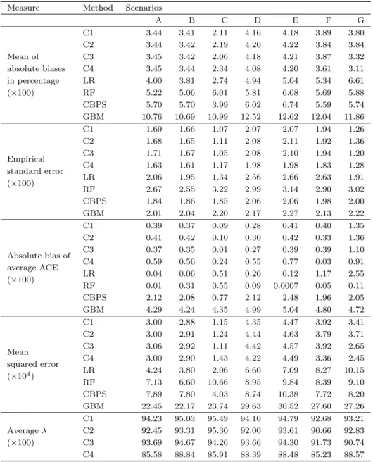
From scenarios A to G, the model averaging methods result in smallest mean of absolute biases in percentage across all scenarios followed by LR, RF, and CBPS. Particularly in scenario G, the mean bias percentage of LR is about twice the size of C4. The GBM method has the largest mean of absolute bias compared to other approaches considered. This shows that the model averaging methods indeed averaged out the biases from LR and RF and increased efficiency in all scenarios.

In almost all scenarios, the empirical standard errors of all model averaging approaches

are less than those from traditional approaches. Figure3.1also shows that the distributions

of the ACE estimates from model averaging methods are more centralized than other methods. The LR and RF methods have more outliers in all scenarios.

The MSE is the sum of the squared bias and the empirical variance. Among all methods examined, the model averaging approaches have the smallest MSE. The GBM method produces the largest MSE in all scenarios.

The coverage rates of 95% confidence intervals are very high for all methods in all scenarios (results not shown). The reason may be because the confidence interval is based

on the theoretical standard error calculated using the sandwich formula in the survey

package in R (Lumley,2004) which is much larger that the empirical standard error (results

not shown). This suggests that the sandwich formula is too conservative. The usage of survey package should be taken cautiously since a design based method is used to construct the variance estimator while our method is model based. Theoretically, it is

a wrong formula to estimate the variance of average causal effect. The survey package

(44)

Table 3.1: Performance of Measures by Propensity Score Models in 1000 Simulated Data Sets withn= 1000 (Estimation of ACE)

Measure Method Scenarios

A B C D E F G Mean of absolute biases in percentage (×100) C1 3.44 3.41 2.11 4.16 4.18 3.89 3.80 C2 3.44 3.42 2.19 4.20 4.22 3.84 3.84 C3 3.45 3.42 2.06 4.18 4.21 3.87 3.32 C4 3.45 3.44 2.34 4.08 4.20 3.61 3.11 LR 4.00 3.81 2.74 4.94 5.04 5.34 6.61 RF 5.22 5.06 6.01 5.81 6.08 5.69 5.88 CBPS 5.70 5.70 3.99 6.02 6.74 5.59 5.74 GBM 10.76 10.69 10.99 12.52 12.62 12.04 11.86 Empirical standard error (×100) C1 1.69 1.66 1.07 2.07 2.07 1.94 1.26 C2 1.68 1.65 1.11 2.08 2.11 1.92 1.36 C3 1.71 1.67 1.05 2.08 2.10 1.94 1.20 C4 1.63 1.61 1.17 1.98 1.98 1.83 1.28 LR 2.06 1.95 1.34 2.56 2.66 2.63 1.91 RF 2.67 2.55 3.22 2.99 3.14 2.90 3.02 CBPS 1.84 1.86 1.85 2.06 2.06 1.98 2.00 GBM 2.01 2.04 2.20 2.17 2.27 2.13 2.22 Absolute bias of average ACE (×100) C1 0.39 0.37 0.09 0.28 0.41 0.40 1.35 C2 0.41 0.42 0.10 0.30 0.42 0.33 1.36 C3 0.37 0.35 0.01 0.27 0.39 0.39 1.10 C4 0.59 0.56 0.24 0.55 0.77 0.03 0.91 LR 0.04 0.06 0.51 0.20 0.12 1.17 2.55 RF 0.01 0.31 0.55 0.09 0.0007 0.05 0.11 CBPS 2.12 2.08 0.77 2.12 2.48 1.96 2.05 GBM 4.29 4.24 4.35 4.99 5.04 4.80 4.72 Mean squared error (×104₎ C1 3.00 2.88 1.15 4.35 4.47 3.92 3.41 C2 3.00 2.91 1.24 4.44 4.63 3.79 3.71 C3 3.06 2.92 1.11 4.42 4.57 3.92 2.65 C4 3.00 2.90 1.43 4.22 4.49 3.36 2.45 LR 4.24 3.80 2.06 6.60 7.09 8.27 10.15 RF 7.13 6.60 10.66 8.95 9.84 8.39 9.10 CBPS 7.89 7.80 4.03 8.74 10.38 7.72 8.20 GBM 22.45 22.17 23.74 29.63 30.52 27.60 27.26 Averageλ (×100) C1 94.23 95.03 95.49 94.10 94.79 92.68 93.21 C2 92.45 93.31 95.30 92.00 93.61 90.66 92.83 C3 93.69 94.67 94.26 93.66 94.30 91.73 90.74 C4 85.58 88.84 85.91 88.39 88.48 85.23 88.57

In each cell, the numbers are multiplied by 100, except for mean squared error, the numbers are multiplied by 10000. C1: Model averaging method with mean ASMD ; C2: Model averaging method with median ASMD; C3: Model averaging method with max ASMD; C4: Model averaging method with mean KS statistic; LR: Logistic regression; RF: Random forest; CBPS: Covariate balancing propensity score; GBM: Generalized boosted model; CI: Confidence interval.

(45)

● ● ● ● ● ● ● ● ● ● ● ● ● ● ● ● ● ● ● ● ● ● ● ● ● ● ● ● ● ●● ● ● ● ● ● ● ● ● ● ● ● ● ● ● ● ● ● ● ● ● ● ● ● ● ● ● ● ● ● ● ● ● ● ● ● ● ● ● ● ● ● ● ● ● ● C1 C2 C3 C4 LR RF CBPSGBM −0.55 −0.50 −0.45 −0.40 −0.35 −0.30 Scenario A ● ● ● ● ● ● ● ● ● ● ● ● ● ● ● ● ● ● ● ● ● ● ● ● ● ● ● ● ● ● ● ● ● ● ● ● ● ● ● ● ● ● ● ● ● ● ● ● ● ● ● ● ● ● ● ● ● ● ● ● ● C1 C2 C3 C4 LR RF CBPSGBM −0.50 −0.45 −0.40 −0.35 −0.30 Scenario B A CE estimates ● ● ● ● ● ● ● ● ● ● ● ● ● ● ●● ● ● ● ● ● ● ● ● ● ● ● ● ● ●● ● ● ● ● ● ● ● ● ● ● ● ● ● ● ● ● ●● ● ● ● ● ● ● ● ● ● ● ● ● ● ● ● ● ● ● ● ● ● ● ● ● ● ● ● ● ● ● ● ● ● ● ● ● ● ● ● ● ● ● ● ● ● ● ● ● ● ● ● ● ● ● ● ● ● ● ● ● ● ● ● ● ● ● ● ● ● ● ● ● ● C1 C2 C3 C4 LR RF CBPSGBM −0.7 −0.6 −0.5 −0.4 −0.3 Scenario C ● ● ● ● ● ● ● ● ● ● ● ● ● ● ● ● ● ● ● ● ● ● ● ● ● ● ● ● ● ● ● ● ● ● ● ● ● ● ● ● ● ● ● ● ● ● ● ● ● ● ● ● ● ● ● ● ● ● ● ● ● ● ● ● ● ● ● ● ● ● ● ● ● ● ● ● C1 C2 C3 C4 LR RF CBPSGBM −0.60 −0.55 −0.50 −0.45 −0.40 −0.35 −0.30 Scenario D A CE estimates ● ● ● ● ● ● ● ● ● ● ● ● ● ● ● ● ● ● ● ● ● ● ● ● ● ● ● ● ● ● ● ● ● ● ● ● ● ● ● ● ● ● ● ● ● ● ● ● ● ● ● ● ● ● ● ● ● ● ● ● ● ● ● ● ● ● ● ● ● ● ● ● ● ● ● ● ● ● ● ● ● ● ● ● ● ● ● ● ● ● ● ● ● ● ● ● ● ● ● ● ● ● ● ● ● ● ● ● ● ● ● ● ● C1 C2 C3 C4 LR RF CBPSGBM −0.55 −0.50 −0.45 −0.40 −0.35 −0.30 Scenario E ● ● ● ● ● ● ● ● ● ● ● ● ● ● ● ● ● ● ● ● ● ● ● ● ● ● ● ● ● ● ● ● ● ● ● ● ● ● ● ● ● ● ● ● ● ● ● ● ● ● ● ● ● ● ● ● ● ● ● ● ● ● ● ● ● ● ● ● ● ● ● ● ● ● ● ● ● ● ● ● ● ● ● ● ● ● ● ● ● ● ● ● ● ● ● ● ● ● C1 C2 C3 C4 LR RF CBPSGBM −0.60 −0.55 −0.50 −0.45 −0.40 −0.35 −0.30 Scenario F A CE estimates ● ● ● ● ● ● ● ● ● ● ● ● ● ● ● ● ● ● ● ● ● ● ● ● ● ● ● ● ● ● ● ● ● ● ● ● ● ● ● ● ● ● ● ● ● ● ● ● ● ● ● ● ● ● ● ● ● ● ● ● ● ● ● ● ● ● ● ● ● ● ● ● ● ● ● ● ● ● ● ● ● ● ● ● ● ● ● ● ● ● ● ● ● ● ● ● ● ● ● ● ● ● ● ● ● ● C1 C2 C3 C4 LR RF CBPSGBM −0.55 −0.50 −0.45 −0.40 −0.35 −0.30 Scenario G

Figure 3.1: Boxplots of ACE Estimates across All Simulation Scenarios (n = 1000 units,

1000 replications)

C1: Model averaging method with mean ASMD as balance statistic; C2: Model averaging method with median ASMD as balance statistic; C3: Model averaging method with max ASMD as balance statistic; C4: Model averaging method with mean KS statistic as balance statistic; LR: Logistic regression method; RF: Random forest method; CBPS: Covariate balancing propensity score; GBM: Generalized Boosted Model.

(46)

too conservative in this case. The use of the bootstrap approach instead of the sandwich formula may yield more reliable confidence intervals. This is the approach we take in

Section3.4.

We also record the absolute bias of the average ACEs over 1000 replications. Among all approaches, the proposed model averaging methods reduced the bias in scenarios F & G, compared to LR, CBPS, and GBM. The RF method produces smallest biases but its empirical standard errors are the largest.

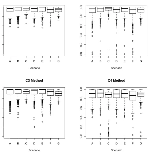
Figure3.2shows the distributions ofλfor C1, C2, C3, and C4 methods from scenario A

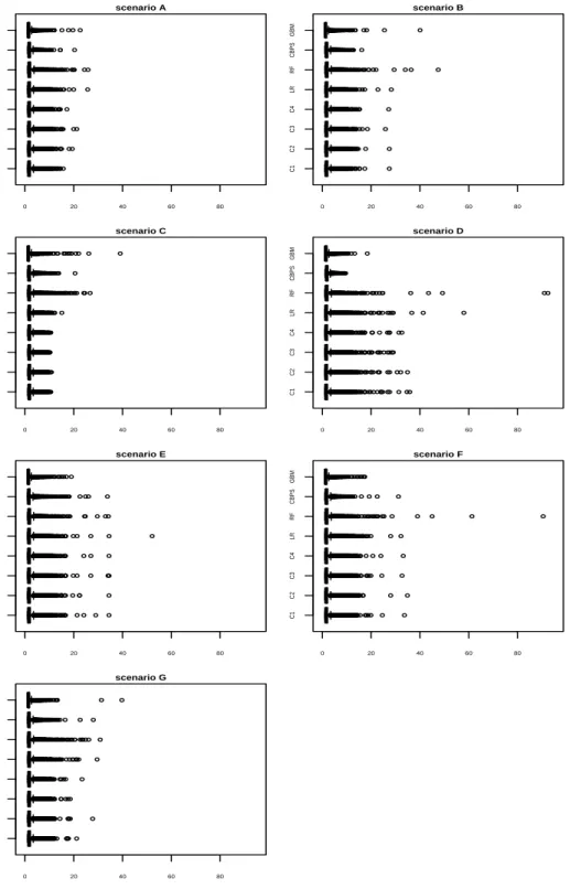
to G. Figure3.3shows the distributions of propensity score weights under different methods

for randomly selected 10 data sets with n = 1000. Heavy or extreme weights can lead to

biased and highly variable estimates of the ACE. Compared to LR and RF methods, the model averaging methods have fewer heavy weights especially in more complex scenarios. The GBM also has fewer extreme heavy weights.

(47)

● ● ● ● ● ● ● ● ● ● ● ● ● ● ● ● ● ● ● ● ● ● ● ● ● ● ● ● ● ● ● ● ● ● ● ● ● ● ● ● ● ● ● ● ● ● ● ● ● ● ● ● ● ● ● ● ● ● ● ● ● ● ● ● ● ● ● ● ● ● ● ● ● ● ● ● ● ● ● ● ● ● ● ● ● ● ● ●● ● ● ● ● ● ● ● ● ● ● ● ● ● ● ● ● ● ● ● ● ● ● ● ● ● ● ● ● ● ● ● ● ● ● ● ● ● ● ● ● A B C D E F G 0.0 0.2 0.4 0.6 0.8 1.0 C1 Method Scenario ● ● ● ● ● ● ● ● ● ● ● ● ● ● ● ● ● ● ● ● ● ● ● ● ● ● ● ● ● ● ● ● ● ● ● ● ● ● ● ● ● ● ● ● ● ● ● ● ● ● ● ● ● ● ● ● ● ● ● ● ● ● ● ● ● ● ● ● ● ● ● ● ● ● ● ● ● ● ● ● ● ● ● ● ● ● ● ● ● ● ● ● ● ● ● ● ● ● ● ● �