Real-Time Scheduling Algorithm Design on Stochastic Processors

(1)

DigitalCommons@USU

All Graduate Theses and Dissertations

Graduate Studies

Spring 2014

Real-Time Scheduling Algorithm Design on

Stochastic Processors

Anushka Pakrashi

Utah State University

Follow this and additional works at:

http://digitalcommons.usu.edu/etd

Part of the

Computer Engineering Commons

This Thesis is brought to you for free and open access by the Graduate Studies at DigitalCommons@USU. It has been accepted for inclusion in All Graduate Theses and Dissertations by an authorized administrator of DigitalCommons@USU. For more information, please contact

[email protected].

Footer Logo

Recommended Citation

Pakrashi, Anushka, "Real-Time Scheduling Algorithm Design on Stochastic Processors" (2014).All Graduate Theses and Dissertations. Paper 2327.

(2)

PROCESSORS

by

Anushka Pakrashi

A thesis submitted in partial fulfillment of the requirements for the degree

of

MASTER OF SCIENCE in

Computer Engineering

Approved:

Dr. Tam Chantem Dr. Ryan Gerdes

Major Professor Committee Member

Dr. Sanghamitra Roy Dr. Mark R. McLellan

Committee Member Vice President for Research and

Dean of the School of Graduate Studies

UTAH STATE UNIVERSITY Logan, Utah

(3)

(4)

Abstract

Real-Time Scheduling Algorithm Design on Stochastic Processors

by

Anushka Pakrashi, Master of Science Utah State University, 2014

Major Professor: Dr. Tam Chantem

Department: Electrical and Computer Engineering

An exciting solution to the power challenges in computing lies in careful relaxations of the correctness constraints of hardware. Recent studies have shown that significant power savings are possible with the use of inexact processors, which may contain a small percentage of errors in computation. However, use of such processors in time-sensitive systems is challenging as these processors significantly hamper the system performance. In this thesis, a design framework is developed for real-time applications running on stochastic processors. To identify hardware error patterns, two methods are proposed to predict the occurrence of hardware errors. In addition, an algorithm is designed that uses knowledge of the hardware error patterns to judiciously schedule time jobs in order to maximize real-time performance. Both analytical and simulation results show that the proposed approach provides significant performance improvements when compared to an existing real-time scheduling algorithm and is efficient enough for online use.

(5)

Public Abstract

Real-Time Scheduling Algorithm Design on Stochastic Processors

by

Anushka Pakrashi, Master of Science Utah State University, 2014

Major Professor: Dr. Tam Chantem

Department: Electrical and Computer Engineering

Recent studies have shown that significant power savings are possible with the use of in-exact processors, which may contain a small percentage of errors in computation. However, use of such processors in time-sensitive systems is challenging as these processors signif-icantly hamper the system performance. In this thesis, a design framework is developed for real-time applications running on stochastic processors. To identify hardware error pat-terns, two methods are proposed to predict the occurrence of hardware errors. In addition, an algorithm is designed that uses knowledge of the hardware error patterns to judiciously schedule real-time jobs in order to maximize real-time performance. Both analytical and simulation results show that the proposed approach provides significant performance im-provements when compared to an existing real-time scheduling algorithm and is efficient enough for online use.

(6)

(7)

Acknowledgments

Having a good advisor might be the single biggest factor in determining the success of a graduate student’s life. And undoubtedly, I found the best. I would like to thank Dr. Tam Chantem for believing in me, for her unwavering support and assistance. This work would never have been possible without her insightful suggestions, willingness to listen, and immense patience.

I am also thankful to my committee members, Dr. Ryan Gerdes and Dr. Sanghamitra Roy, who had a big impact on the quality and scope of my research. I am grateful for their earnest support.

Any thesis is a cumulation of immense effort over a long period of time. I am extremely thankful for having people around me who made my graduate life easier. There is simply no way in which I could have completed this thesis without my parents, who always had faith in me and allowed me to pursue my interests from the very beginning.

I would also like to thank Abhisek, who has been a pillar of support in my life for all these years. He has always been the first person to congratulate me on my success, and his stern rebuke helped me think straight in times of need.

This acknowledgment will remain incomplete without mentioning all my friends from Logan and Salt Lake City who helped me balance work and fun. Finally, I am also extremely thankful to my friends from India for constantly motivating and supporting me during odd hours of the day over instant-messenger.

(8)

List of Tables

Table Page

4.1 An example with two frame-based tasks. . . 11 4.2 An example with three periodic tasks. . . 13

(11)

List of Figures

Figure Page

3.1 System model. . . 9

4.1 (m,k) record of a frame-based task. . . 12

4.2 Timeline showing execution and deadline misses of the frame-based tasks in Table 4.1. . . 12

4.3 Timeline showing execution pattern of example task set. . . 13

4.4 Timeline showing job swap in example task set. . . 14

5.1 Histogram showing number of errors for 1% error. . . 17

5.2 Average number of errors per simulation for 1% error. . . 17

5.3 Average number of errors for 1000 time units as a function of hardware error percentage. . . 18

5.4 Poisson distribution pdf. . . 19

5.5 Error localization. . . 20

5.6 Error-prone zone based on the Poisson distribution approach. . . 21

5.7 Error-prone zone based on the error localization approach. . . 22

6.1 Algorithm flowchart. . . 25

6.2 Average case. . . 29

7.1 Average percentage of (m,k) misses in the worst case. . . 31

7.2 Average percentage of (m,k) misses in the best case. . . 32

7.3 Average percentage of (m,k) misses in the average case. . . 32

7.4 Percentage decrease in (m,k) misses with increase in error percentage. . . . 33

7.5 Percentage decrease in (m,k) misses with increasing utilization. . . 33

7.6 Percentage decrease in (m,k) misses over a given time period using error localization in best case. . . 33

7.7 Percentage decrease in (m,k) misses over a given time period using error localization in average case. . . 34

7.8 Percentage decrease in (m,k) misses over a given time period using error localization in worst case. . . 34

(12)

Acronyms

ATM automated teller machine

QOS quality of service

VLSI very large scale integration

CMOS complementary metal oxide semiconductor

GPU graphics processing unit

(13)

Chapter 1 Introduction

This chapter presents a brief overview of real-time systems and introduces readers to various challenges faced by such systems due to physical constraints. With technology scal-ing, as power savings becomes an important consideration, the use of inexact processors is becoming more and more relevant and important in the computer architecture and system design communities. However, usage of such processors in real-time systems may consid-erably hamper the real-time performance. In this thesis, a design framework is proposed for real-time systems running on stochastic processors. Specifically, the hardware error pat-terns are identified and an efficient algorithm is developed to effectively reschedule real-time jobs to maximize some performance metric, to be defined later. Simulation results show that the proposed method can increase real-time performance by 62% on average and up to 79%.

1.1 Brief Overview of Real-Time System

An embedded real-time system is a computer system designed for specific functions within a larger system. It can be thought of as a special kind of computing system where timeliness plays an important role along with correct functionality. A real-time system must guarantee correct response within certain time constraints which are often referred to as deadlines. An automated teller machine (ATM) is an example of a real-time system; when an ATM machine is used, there is a certain time limit within which complete service is expected. There lies the timeliness requirement of a real-time system.

Real-time systems can be categorized into three types: hard, firm, and soft. In a hard real-time system, missing a deadline could result into catastrophic consequences and can be referred to as total system failure. Hence, absolutely no deadline misses are allowed in

(14)

such systems.

In the case of firm real-time systems, missing a deadline is not detrimental to the entire system performance. However, too many deadline misses may lead to systems that do not meet their performance requirements, e.g. a control system may become unstable.

For soft real-time systems, tasks may be completed late without considerably hamper-ing the system’s performance level. Nevertheless, it is important to ensure that as many deadlines are met as possible to maximize the quality of service (QOS). Example of such system is an online video streaming application. In this thesis, the focus is on soft real-time applications.

There are many real-time applications in which it is not necessary for every job to meet its deadline. The transmission of frames in a video application can be considered one such example. Here, a few missed deadlines can be tolerated as long as they are under a maximum allowable loss percentage. However, even then the quality of the video stream will not be acceptable if there are several consecutive deadline misses. For example, consider the following scenarios: (i) 1 out of 10 deadline misses, and (ii) 100 deadline misses followed by 900 deadlines met. For both scenarios, the miss percentage is 10, but it is clear that both may lead to unequal performance levels. Thus, for some applications the deadline misses must be adequately spaced. This generates the notion of (m,k)-firm deadlines. The requirement is expressed by specifying two constants m and k such that the QOS of the application is acceptable if at least m jobs in any sliding window of k consecutive jobs meet their deadlines. When fewer than m jobs meet their deadlines out of k jobs, the task set is said to have experienced a dynamic failure.

1.2 Stochastic Processors

Real-time applications are slower to adapt new technologies, but as power savings become an important design challenge, the use of non-traditional processors must be con-sidered. Although Moore’s law has accurately predicted the trend for the very large scale integration (VLSI) industry in the past decades, technology scaling is reaching its limits. Increase in chip power density has become a major problem. According to Intel Vice

(15)

Presi-dent Patrick Gelsinger, “If scaling continues at present pace, by 2005, high speed processors would have power density of nuclear reactor, by 2010, a rocket nozzle, and by 2015, surface of sun.”A very recent concept that provides a solution for the scaling and power density prob-lems is the concept of inexact chip. Researchers found that power and resource efficiency can be improved if occasional errors are allowed in the chip. It was shown that traditional complementary metal oxide semiconductor-based (CMOS-based) design consume too much power since they are always designed to perform correctly. Moreover, designing perfect hardware is expensive. If there were a way to systematically introduce errors in the chip, we could save cost while reducing waste during chip inspection. Recent research shows that 30% power can be saved in an OPENSPARC processor if the error-rate is increased by 2% [1,2]. The current error rate is about 1% but it is expected to increase, especially with post-CMOS and nano-scale technologies [3]. Using these so-called stochastic processors, extremely low-power designs are possible.

1.3 Problem Statement

While stochastic processors can be used in applications that are naturally tolerant to errors, a graphics processing unit (GPU) application for example, their use in real-time systems is a challenge. Timeliness and correct functionality, the main features required by real-time systems, may hamper the use of stochastic processors due to the occasional occurrence of errors. However, it is observed that some real-time systems have less strin-gent timing requirements which can be exploited in order to save energy and cost without sacrificing performance. Since real-time systems are traditionally over-designed, for the worst-case operating scenarios, potential energy and cost benefits are large.

In this thesis, the following main contributions are made.

1. To be able to provide error resilience in real-time systems, predictions must be made regarding when an error may occur. Two methods are proposed to accomplish this step. The first method involves predictions by fitting hardware errors to some well-known probability distribution. In the second method, the hardware error is localized

(16)

based on the probability of error occurrence.

2. A scheduling algorithm is designed that rearranges real-time jobs in such a way that fewer jobs miss their deadlines and the QOS of the application is improved.

3. Finally, extensive performance evaluations are conducted to show that the proposed algorithm consistently performs better than an error-ignorant algorithm. Even in the worst case scenario, the performance of this algorithm is never worse than that of the existing (m,k) algorithm. The proposed algorithm performs better than the existing algorithm 90% of the time on an average.

(17)

Chapter 2 Related Work

The concept of stochastic processors were initially introduced by T. Austin et al. [4]. Recent research [5,6] suggests that significant energy and power savings are possible if the constraint on correctness is relaxed in processors. Most existing approaches propose error-tolerant design at the architectural level, and not at the system level. Kahng et al. propose a recovery-driven design approach which optimizes the processor for a target timing error-rate [5]. Through a series of experiments, they have shown that significant power savings can be obtained for similar performance level. Power savings increase to as high as 28% for a 4% error-rate. Errors are either detected or corrected by a hardware error tolerance mechanism. Similar work was done to create error-tolerant design which operates by optimizing the critical path during the course of its operation [6-8]. Kahng et al. propose a method to perform power-aware slack redistribution, which is another design-level approach that reallocates timing-slack in a power and area-efficient manner [2]. In this approach it was shown that 29% power reduction is possible by increasing the error rate to just 2%.

Shanbhag et al. propose an estimator block - a computational block which is of much lower complexity (typically 5%-20%) than the main block [9]. The main block is allowed to make errors, whereas, the estimator block generates some statistical estimations to correct the main output. This gives an approximate detection and correction of the error. Another method proposed in this paper was computation with error statistics. This too requires a detector or voter to determine the output. However, in both the cases, to implement such a system, extra hardware is required which increases the cost as well as the delay of the system.

(18)

Sloan et al. present algorithmic fault correction [10]. They have proposed three ap-proaches, the first of which relies on relaxing the correctness of the application based upon an analysis of application characteristics. The second approach relies upon detecting and correcting the errors within a specific application as they arise. Finally, the third approach transforms applications into more error-tolerant forms. In this work, the faults are at first detected and then corrected within the algorithm. Although the proposed algorithm has low overhead for low error rates, it may be too costly for systems with higher error rates. When the error rate increases, the overheads incurred from the re-computation and correction increases.

There is also active research going on to design a scalable stochastic processor [11]. Scalable architecture in a processor is designed by replacing or supplementing traditional functional units with gracefully degrading units. The authors have proposed a comput-ing platform for error-tolerant applications which can provide stochastically correct results and scale its performance according to the power-constraints. This is accomplished by dynamically switching among multiple functional units according to varying performance requirements. This method too requires extra hardware in the system.

In terms of fault-tolerant real-time system design, although stochastic processors have received significant research attention [8,12-26], very few existing works focused on hard-ware error predictions. Error introduced by hardhard-ware in a system with timing constraints can cause severe consequences or, at the least, very degraded performance. Part of this thesis focuses on designing an algorithm which predicts the hardware error occurrence by mapping it to various probability distribution functions. Zhu proposes reliability-aware en-ergy management schemes which dynamically schedule recoveries for tasks which are scaled down to recuperate the reliability loss due to energy management [27]. This is a different approach to achieving energy efficiency and does not account for hardware errors. The concept of checkpointing is proposed to achieve fault-tolerance and power management in real-time systems [28-34]. The concept of checkpointing, where the system rolls back to the nearest checkpoint if a fault is detected, is similar in each approach. Although many

(19)

schemes for checkpointing are proposed, every scheme involves re-execution. In contrast, the natural resilience of soft real-time systems is exploited in this work, to provide fault tolerance without additional hardware nor re-executions.

In soft real-time systems, a few deadline misses are tolerable as long as such misses are not consecutive and are sufficiently spaced. Several models have been proposed to deal with such systems. An example is the (m,k) model, proposed by Hamdaoui and Ramanathan [35]. A real-time stream or task is said to have (m,k)-firm deadline if at least m out of k consecutive jobs meet their deadlines in every sliding window. If the number of deadline misses exceeds m out of k, then dynamic failure occurs. Ramanathan proposed the concept of distance-based priority assignment which results in a reduction in the probability of dynamic failure [36]. However, none of the algorithms associated with the (m,k) model or other job skip models such as dynamic window-constrained scheduling [37] or skip-over model [38] consider the possibility of errors during job executions. For example, if hardware error effects in any one of the m out of k jobs which have met their deadlines, dynamic failure may occur. The proposed algorithm aims to address this problem.

(20)

Chapter 3 Preliminaries

3.1 System Model

Consider a task set where each task τi is described by a release time Ri, worst-case execution time Ci, periodTi, and relative deadlineDi, where Di ≤Ti. The tasks are non-preemptable in nature. In addition, each task has an (m,k)-firm requirement which means that m out of every k consecutive tasks must meet their deadline in order to avoid dynamic failure. In the absence of hardware errors, all tasks meet their (m,k)-firm requirements.

The notion of the (m,k)-firm deadlines is quite general. Every job from a task set must meet its deadline if the (m,k) requirement is (1,1). Similarly (1,2) corresponds to the situation where every alternate job must meet their deadlines in a task stream. It is also important to note that apart from ensuring that the deadline misses are adequately spaced, the maximum allowable loss rate of a stream with (m,k)-firm requirements is determined by (k−m)/k. For example, although both (3,4) and (6,8) imply a 25% allowable loss rate, the former one has a more stringent timing requirement since no more than one consecutive job can miss its deadline in a given window.

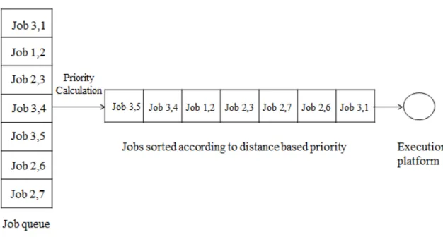
Figure 3.1 represents the system model for the real-time system under consideration where there are seven jobs from three different tasks. Jobs from different tasks are arranged in the job queue according to a first-come first-serve basis. Job (1,2) represents the 2nd job of task 1. The priority of each job is then calculated according to the distance-based priority (DBP) algorithm, which will be described in the next section and the jobs are sorted from highest priority to lowest priority, an order in which they are serviced.

3.2 Distance-Based Priority Assignment Algorithm

(21)

Fig. 3.1: System model.

deadlines missed and met in the current window. A job that has been serviced by the application may either meet or miss its deadline. The technique requires the stream to remember the output of its last (k−1) jobs.

A stream is closer to dynamic failure if its job misses a deadline. The objective of the DBP algorithm is to prevent the tasks from experiencing dynamic failures. In this approach, if a task stream is close to dynamic failure, a higher priority is assigned to its next job. This will increase the chance of the job meeting the deadline and thus move the task stream away from dynamic failure. The priority value that is assigned to each job is the minimum number of consecutive failures required to take the task stream from current state to failure state. Jobs with lower priority values have higher priority in receiving service. For example, a job with priority value of 3 have to experience three consecutive deadline misses for its task stream to reach the failure state, whereas a job with priority value of 1 has to experience just one more deadline miss to experience dynamic failure. For this reason, the job with a lower priority value is given a higher priority so that it has a better chance of meeting its deadline. This is done at the cost of other tasks which can afford a

(22)

few deadline misses. For jobs with the same priority value, ties are broken in favor of the jobs with earlier deadlines. The DBP algorithm is shown in Algorithm 3.1.

Algorithm 3.1DBP (τi)

Input:

task (τi) with (m, k) values (mi, ki), i= 1, ..., n

Output:

priority, Pi,i= 1, ..., n

Lethmp τi be a hashmap that contains the last (k−1) outputs for task ,τi

sum of scores← 0

for each task τi ∈ Γdo

foreach element ∈hmp τi do

sum of scores=sum of scores+hmp Ti.get(element)

End for End for

(23)

Chapter 4 Motivating Example

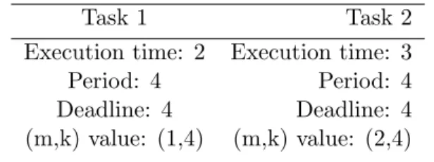
To demonstrate the need for an error-aware algorithm, consider an example consisting of two tasks with the same period, and deadlines as shown in Table 4.1.

The (m,k) value represents (m.k)-firm deadline requirement for a task. A real-time task is said to have (m,k)-firm deadline if at least m out of any k consecutive jobs meet their respective deadlines. If fewer than m out of k jobs meet their deadlines, then the QOS for that particular task is said to have fallen below an acceptable limit and that task experiences dynamic failure. The (m,k) value of task 1 is (1,4), which means that at least 1 out of every 4 consecutive jobs must meet its deadline. In Figure 4.1, the (m,k) record for the first five jobs of both tasks is shown, based on the DBP scheduling algorithm. The tick indicates successful completion of a job and the cross indicates a deadline miss. In case of task 1, if a hardware error occurs during the execution of the 5th job, task 1 will experience dynamic failure.

More details regarding the job executions are provided in the following section. At time 0, both the tasks have the same priority. The execution is non-preemptive in nature. At time 4, job 1 of task 2 misses its deadline and at time 12, job 2 of task 1 misses its deadline. The timeline of this event is represented in Figure 4.2.

An error-prone zone is defined as a time interval with the maximum probability of occurrence of hardware error.

Table 4.1: An example with two frame-based tasks.

Task 1 Task 2

Execution time: 2 Execution time: 3

Period: 4 Period: 4

Deadline: 4 Deadline: 4

(24)

Fig. 4.1: (m,k) record of a frame-based task.

Fig. 4.2: Timeline showing execution and deadline misses of the frame-based tasks in Table 4.1.

(25)

In the example shown in Table 4.1, assume that, time 18 is the end of the error-prone zone. The dynamic failure experienced by task 1 can be avoided if the execution of task 1 can be moved to 18, as long as task 1’s original deadline is after time 18.

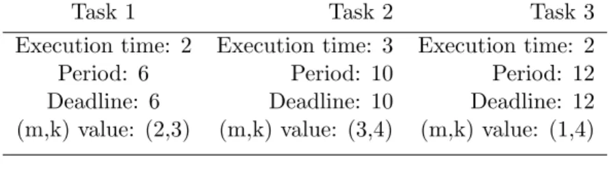
Consider another example consisting of three task sets which have different deadlines and periods as shown in Table 4.2. It is shown that a hardware error, if not treated properly, may cause dynamic failure irrespective of the number of tasks in the task set or the nature of task sets, i.e. whether it is a frame-based or a periodic task set.

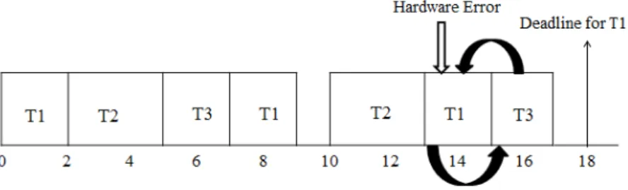
This example also follows the DBP scheduling policy. Figure 4.3 illustrates the execu-tion pattern of task 1, task 2, and task 3.

According to Li et al. [3], the hardware error occurrences follow the Poisson process. After modeling the proposed system, it was found that time interval between 0-15 time units is an error-prone zone in this example.

In this case, if hardware error occurs at time slot 15, job 3 of task 1 may have an erroneous output which leads to degraded QOS. If it is possible to swap job 3 of task 1 and job 2 of task 3, task 1 is prevented from experiencing dynamic failure without hampering the status of task 3. Figure 4.4 gives a detailed representation of the process discussed above.

Table 4.2: An example with three periodic tasks.

Task 1 Task 2 Task 3

Execution time: 2 Execution time: 3 Execution time: 2

Period: 6 Period: 10 Period: 12

Deadline: 6 Deadline: 10 Deadline: 12

(m,k) value: (2,3) (m,k) value: (3,4) (m,k) value: (1,4)

(26)

(27)

Chapter 5 Identification of Error-Prone Zones

5.1 Overview

Consider a real-time system with some (m,k)-firm requirement, the attributes of which were discussed in Chapter 3. It has been shown in previous work that using stochastic processors and relaxing the hardware correctness results in significant power benefits. How-ever, since one of the main requirements of a real-time system is correct functionality, the use of stochastic processors may have adverse effects on the performance of a real-time system. Here the system under consideration is a real-time system with (m,k)-firm deadline requirement. As shown in previous chapters, the DBP algorithm follows a sliding window protocol. This means that m out of k jobs must meet their deadline in each consecutive window.

In order to proactively handle hardware errors at runtime, it is required to predict when errors may occur. While it is impossible to determine exactly when the hardware error is about to occur, it is feasible to predict the time intervals, i.e. zones which have maximum probability of hardware errors. It would then be possible to tolerate errors dynamically without adding hardware or re-executing tasks. Two separate approaches of determining error-prone zones are proposed and discussed in this section.

5.2 Poisson Distribution Approach

The actual probability distribution that hardware errors follow is debatable. In this work, it is assumed that the error occurrences follow Poisson process. In probability theory and statistics, the Poisson distribution is a discrete probability distribution that expresses the probability of a given number of events occurring in a fixed interval of time and/or space if these events occur with a known average rate and independently the time since

(28)

the last event. If only the average rate given, and knowing that the process is completely random in nature, the Poisson distribution specifies the probability of the system under consideration for a certain instance. Let the probability of occurrence of hardware error be P. Then according to Poisson distribution, the probability that k errors happen is given by Equation (5.1).

Pλ,T (X=k) =

e−λT(λT)k

k! , (5.1)

whereλis the average number of errors over a time period T.

If the value ofλis known, it is straightforward to calculate the probability of having k errors.

No existing work assumes that λ is known. To find the value of λ, the concept that is proposed is that of a histogram. To simulate 1% hardware error, random numbers were generated between 1 and 100 and whenever the answer was 1, it was considered to be erroneous. This simulation was run for 100,000 times to determine a pattern of occurrence of 1s if it existed. A histogram was constructed with 100 columns, each of which had 1,000 datapoints. The height of each column was determined by the number of jobs that were affected by hardware errors within that range. This experiment was also conducted with 10, 100, and 10,000 datapoints, but 10 and 100 datapoints were not enough to represent the true nature of the distribution. Also, the mean determined from 10,000 datapoints was 49.95 which is 10 times the mean derived from 1000 datapoints. Therefore, for simplicity, we use 1,000 datapoints for constructing the histogram.

Figure 5.1 is a part of the histogram, where each column has 1000 datapoints and the y-axis represents the number of errors occurring in that interval. The mean was then calculated from the datapoints and 10,000 such simulations were run. The main idea behind this was to get an unbiased value ofλ.

The average number of errors obtained from the simulation is shown in Figure 5.2. It was observed that the mean value varies between 4.7 and 5.1. To improve accuracy, the mean of means was calculated, the value of which was determined to be 4.995. An important

(29)

Fig. 5.1: Histogram showing number of errors for 1% error.

(30)

assumption made here is that one job having error is equal to one time slot. This means that probability of x jobs having error can be translated into probability of error in x time units. This assumption is required to determine a time period having high probability of error.

This calculation was done to find out λassuming that the hardware error percentage is 1. The same procedure was repeated to obtain the average number of errors when the hardware error percentage was 2.

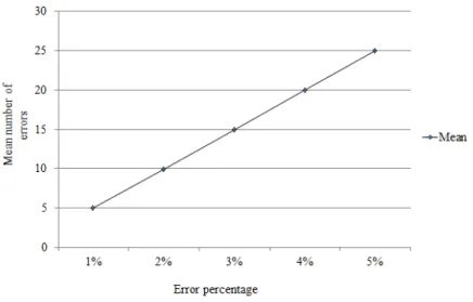
Figure 5.3 shows an interesting property of λ. With an increase in error percentage, the mean also increases proportionally, i.e. for 1% error the mean was calculated to be 4.995, for 2% error it was calculated as 9.99, for 3% error it was 14.997, and so on.

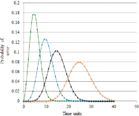
Having calculated these values, the Poisson distribution curve is not difficult to con-struct. Figure 5.4 shows that Poisson curves for 1%, 2%, 3%, and 5% hardware error. The green curve represents the probability of error for 1% hardware error, the blue curve is for 2%, the black is for 3%, and the red curve is for 5% hardware error. It can very well be shown that the error becomes more distributed in the system with increase in hardware error percentage.

Fig. 5.3: Average number of errors for 1000 time units as a function of hardware error percentage.

(31)

Fig. 5.4: Poisson distribution pdf.

5.3 Error Localization Approach

Error localization is the other approach proposed in this thesis in addition to the Poisson distribution approach. This approach is mostly based on a few assumptions derived from experimental data. While the Poisson distribution pdf in Figure 5.4 suggests that the highest probability of error lies in the first few time slots, the error-prone zones determined by this method are more distributed. Testing the proposed algorithm with such an error-prone zone will produce more unbiased and general results.

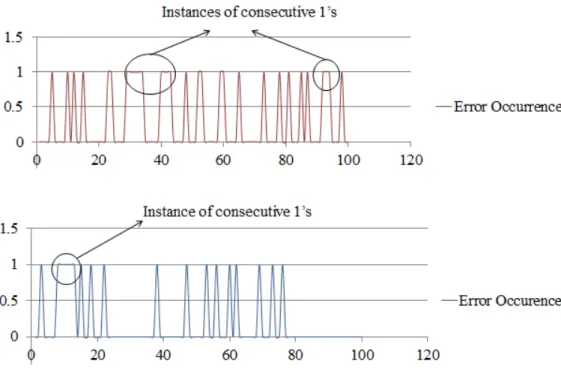
Once the average number of errors per 1,000 instances is determined, the number of errors in each column of the histogram can be checked with respect to the calculated mean value. The height of each column, which determined the number of errors in that interval, is either greater than or less than the calculated mean value. If the height of a column is less than the average number of errors, then the column is denoted as 0 and if the height is greater than or equal to the mean error, then it is denoted as 1. For example, consider

(32)

1% error probability. If the height of the column is less than 4.995, then it is denoted as 0, otherwise it is denoted as 1. This assumption is based on the fact that if the number of errors is less than 4.995 out of 1,000, then it is negligible and can be ignored. Similar experimentation was done for 2%, 3%, and 5% error probability.

The error patterns are plotted and the areas with maximum consecutive occurrence of 1 are separated out. The positioning of the two major error occurrence zones that were separated out after 100,000 simulations is shown in Figure 5.5.

5.4 Selecting the Appropriate Approach

After carefully examining the results, the error-prone zones for both approaches are determined. Figure 5.6 shows the zones having high probability of error if the Poisson distri-bution approach is used. For 1% error, high probability zone ranges from 1 to 15 time units in the first 1000 instances. It is interesting to note that the mean increases proportionally if the granularity of the histogram is increased. This pattern keeps on repeating for the rest of the execution time.

(33)

Fig. 5.6: Error-prone zone based on the Poisson distribution approach.

Figure 5.7 describes the error-prone zone for the second approach. It is determined that out of 1000 datapoints, consecutive errors occur between 95 and 120, 290 and 335, 404 and 421, and 920 and 940 time units. The error-prone zone differs from the previous approach because this is mostly based on experimental results and the previous approach was based on the characteristics of Poisson process.

If a system has unknown error pattern, it is proposed to start execution considering that the error follows Poisson process. The output of the system is monitored to model an error pattern online and switch to error-localization approach when there is enough data.

It is now possible to identify the error-prone zones for both cases discussed above. This will be required in the scheduling algorithm discussed later in the thesis.

(34)

(35)

Chapter 6 Proposed Algorithm

We are interested in solving the following problem.

Problem Statement:

Given the time period having the probability of occurrence of hardware errors, design a scheduling algorithm for real-time systems with (m,k)-firm deadline requirements, so that the QOS is maximized. This means that the algorithm will have to be designed in a way such that jobs with higher priorities, i.e. jobs that are closer to dynamic failure, are less affected by hardware errors.

For real-time systems with (m,k)-firm deadline requirements, the priority of each job is calculated on the basis of its closeness to dynamic failure as discussed in Chapter 3. This concept of job scheduling is taken one step further by considering the problem of hardware errors.

The main idea behind the proposed algorithm is to attempt to move as many jobs as possible out of the error-prone zones which will help to decrease the total number of (m,k)-firm deadline misses in the system. Here, the priority of a job is determined by its closeness to dynamic failure. In other words, a job is said to have a higher priority if it is close to missing its (m,k)-firm deadline requirement. If a high priority job executes during the error-prone zone, it may produce erroneous output in spite of meeting its deadline. This will lead to dynamic failure of that job that would have otherwise met its deadline if the program was running on an error-free processor. However, it is important to design the algorithm in such a manner so that the re-scheduling of the jobs does not hamper the execution of the remaining jobs in the priority queue. A few factors like deadline, priority, and execution time must be accounted for while re-scheduling the jobs. It is worth mentioning, that although the proposed system is modeled in a way that it replicates the original system to

(36)

a great extent, the occurrence of hardware errors is still completely random in nature and it may take place at a few instances out of the determined error-prone zones. Here, the main focus is on the actions to be taken during error-prone zones.

This idea is clearly discussed in the flowchart in Figure 6.1 It is assumed that before the beginning of the first error-prone zone, the scheduler follows the DBP algorithm as discussed in Chapter 3.

6.1 Algorithm Description

At first, it is assumed that the ready jobs in the job queue are sorted according to the DBP algorithm as discussed previously. Since, each task in the task set has a deadline that is less than or equal to its period, there will never be more than one job of the same task in the job queue at the same time.

Once the system enters an error-prone zone, each job in the job queue is checked starting from the highest priority job. At first, the end of the error-prone zone is located and it is checked whether for the highest priority job can be moved to execute after the end of the error-prone zone. The job is next analyzed to determine whether it can be moved to a separate array A, which is to be executed after the end of the error prone zone. In other words, if the array A is non-empty, then the jobs are sorted in the order of non-decreasing deadlines and the time-demand analysis is performed which is given by Equation (6.1). For example, assume that we already have jobs j1 and j2 in the array A having deadlines d1

and d2 respectively. If d1 < d2 then the first job in the array is j1. To be clear, the array

A will be sorted in a non-decreasing order of deadlines.

i

X

j=1

cj ≤di ∀i= 1, ...., n, (6.1)

where c represents the execution time of the job and d represents the deadline.

The time-demand analysis checks if all existing jobs in array A will remain schedulable with the addition of the new job. If both the conditions are satisfied, then the job is moved to the array A. In the next step the algorithm checks to see if the program is still in the

(37)

Enters error-prone zone

Checks whether the end of the error-prone zone + its execution time < its deadline

(1)

Finds the job with highest priority in the array

Array of jobs sorted according to dynamic priority calculation based on their (m,k) values

If yes

Move the job to array, A

Continue executing the remaining jobs in

the array If no

If no

Check for any new job arrival Check if the sum of the execution

time of all existing jobs in array A < = maximum deadline

(2)

Checks whether it is still in error-prone zone If yes

Continue executing normally If no

If condition (2) is met, add it to array A, otherwise drop

the lowest-priority job

Execute using earliest deadline first (EDF) if array A still

has jobs

(38)

error-prone zone and repeats the previous steps until it is out of error-prone zone or the job queue is empty, i.e. there is no new job ready for scheduling.

If any job fail to satisfy any one of the conditions discussed above, then it is kept in the existing job queue for execution. After moving all eligible jobs to array A, the remaining jobs are executed within the error-prone zone according to the DBP algorithm. At every scheduling point, the existing job queue is examined to see if there is a new job arrival. Whenever a new job arrives while the program is still in error-prone zone, it is checked for both the conditions and moved to array A if it satisfies both, otherwise, it is executed within the error-prone zone. At this point it is important to mention that the jobs in array A will be executed using Earliest-Deadline First (EDF) algorithm [39] as it is required to execute the maximum number of jobs after error-prone zone.

As soon as the program is out of the error-prone zone, jobs in array A start executing. Here too, the job array is checked to see if there is a new job arrival. If a new job arrives while array A is non-empty, it is first checked with the time-demand analysis for all the remaining jobs in A. The goal is to execute the maximum number of jobs which will in turn reduce the number of (m,k)-firm deadline misses. Therefore, if the new job fails the time-demand analysis, its priority is compared with the priority of the existing jobs in the array and the least priority job is dropped. The feasibility of the jobs are re-checked before the new job is added to the array. This priority is based on its closeness to dynamic failure. Once array A is empty, the program follows the DBP scheduling algorithm until the arrival of the next error-prone zone.

6.2 Performance Analysis

A comparative performance analysis of the proposed algorithm and the DBP algorithm is conducted to determine if the proposed algorithm ever performs worse than the DBP algorithm. Assume that there are n time slots within the error-prone zone. To find the worst case performance of the proposed algorithm, each time slot is considered to be equal to one job. Therefore, it is considered that there are n jobs in the error-prone zone. This translates as the worst case scenario because the goal of this analysis is to minimize the

(39)

number of jobs being affected by hardware error which will in turn decrease the total number of (m,k) failures. The difficulty increases with increase in number of jobs within the error-prone zone. However, this is an over-estimation as it is nearly impossible to have error in every consecutive time unit.

There are three cases: • Best case,

• Worst case, • Average case.

The goal of this analysis is to show that the proposed algorithm never performs worse than the DBP algorithm.

6.2.1 Best Case

The best case scenario for the proposed algorithm is when each and every job in the error-prone zone can be re-scheduled after the completion of error-prone zone. As it is already assumed that none of the jobs have their period before their deadline, there will not be any arrival of new jobs until all jobs in array A are executed. This will have a 100% better performance than the DBP algorithm. This is because in worst case, if DBP is used, all n jobs might fail while in error-prone zone. But using the proposed algorithm, it is possible to re-schedule all the jobs.

6.2.2 Worst Case

The worst case scenario for the proposed algorithm is when none of the jobs in the job queue can be re-scheduled after the completion of error-prone zone. This will mean that, every job has to be executed using the DBP algorithm and in the worst case, all n jobs might fail. Thus, the proposed algorithm performs similar to the existing DBP algorithm in the worst case.

(40)

6.2.3 Average Case

Figure 6.2 shows the average case, where x out of n jobs get executed within the error-prone zone and the rest (n−x) jobs are re-scheduled. There are three cases that need to be considered:

• Value ofx= n₂,

• Value ofx > n₂,

• Value ofx < n₂.

In the first case, n₂ jobs are executed within the error-prone zone and the rest (n₂ jobs) are re-scheduled. This means that all n₂ jobs in the error-prone zone might fail in the worst-case scenario. After the end of the error-prone zone, new jobs from the already executed task sets might be arriving. In the worst case, all the n₂ tasks have new jobs coming in. If it is not possible to accommodate the new jobs in the re-scheduled job array, then n₂ jobs having the least priorities are dropped. Therefore, total number of failures in this case is

n

2 +

n

2 =n, which is not worse than the existing algorithm.

In the second case,x jobs execute during the error-prone zone and in the worst case, allxjobs might fail. After the end of error-prone zone, there might bexnew jobs in the job queue. Consider that none of the new jobs can be accommodated in the re-scheduled job array. Therefore, at most, all (n−x) jobs are dropped since (n−x)< x. Total number of failures even in this case isx+ (n−x) =n, showing that the performance of this algorithm is same as DBP algorithm in this case.

Finally, in the third case, there arex jobs executing during the error-prone zone and in the worst case, all of them fail to execute successfully. While executing the re-scheduled array A, there might be x new jobs coming in and this might be followed with dropping of x jobs from the queue as discussed previously. Therefore, in this case, total number of failures is (x+x) = 2x. This is better than the DBP algorithm as 2x < n since, x < n/2.

Here, it is assumed that no new job comes in during the error-prone zone. If y new jobs come in, then the total number of job failures using the DBP algorithm will be (n+y).

(41)

Fig. 6.2: Average case.

This is because, the error-prone zone contains n time slots, which means any new job that comes in during this time period have to be dropped if it cannot be re-scheduled. This will similarly translate to the proposed algorithm showing that the number of failures in worst case is never more than (n+y).

The time complexity of the algorithm is O(n.(logk) +n), where nis the total number of jobs at some time instant andkis the number of tasks in the system.

(42)

Chapter 7 Simulations

The effectiveness of the proposed algorithm is compared against the DBP algorithm using simulations. Actual experiments were not performed since hardware errors need to be systematically introduced. Although the proposed techniques were used to determine the error-prone zones, the proposed algorithm does not depend on the actual mechanism with which error-prone zones are determined. The time period having highest possibility of error serves as an input parameter. To ensure fair comparison, both algorithms are run in the same environment with the same number of tasks and occurrences of error.

7.1 Simulation Framework

Since the objective of the simulations is to evaluate the performance of the proposed algorithm compared to the baseline algorithms, it is ensured that identical task sets are executed using the two algorithms and the total number of (m,k)-firm deadline misses is recorded.

Twenty thousand benchmarks were randomly generated, each of which is a task set whose execution time varies between 1 and 5 time units, relative deadline varies between 5 and 15 time units, period varies between 5 and 20 time units, and (m,k) values vary between (1,2) to (9,10). All parameters were randomly generated using uniform distributions to ensure fair analysis. The simulations were conducted on an Intel i7 3.50GHz with 16GB memory.

7.2 Results

From the following data, it is clear that the proposed method achieves the best perfor-mance in terms of decrease in average number of (m,k) misses.

(43)

Fig. 7.1: Average percentage of (m,k) misses in the worst case.

Figure 7.1 shows the average percentage of (m,k) misses in the worst case as a function of error percentage. It is quite evident from the graph that the proposed algorithm never performs worse than the existing (m,k)-firm algorithm. In addition, as the error percentage increases, even in the worse case, the proposed method performs up to 40% better than the DBP algorithm.

In the best case scenario, shown in Figure 7.2, the performance of the proposed algo-rithm improves to 79% better than the existing algoalgo-rithm. On an average, the performance is almost 62% better as shown in Figure 7.3.

The percentage decrease in (m,k) misses as a function of increase in error percentage is shown in Figure 7.4. Figure 7.5 represents the average decrease in percentage of (m,k) misses as a function of system utilization. Although the normalized number of (m,k) misses monotonically increases with an increase in utilization, simulation data show that the max-imum decrease in percentage (≈70%) is achieved when utilization is between 1.2 and 1.5. However, even for very high or very low utilization, the decrease in percentage is never less than 30%, which means the proposed method has at least 30% fewer (m,k) misses than the existing (m,k)-firm algorithm.

(44)

Fig. 7.2: Average percentage of (m,k) misses in the best case.

in best case using error-localization approach. The maximum decrease in percentage for this method is 86.88%. Figure 7.7 and Figure 7.8, respectively, represent the percentage decrease in (m,k) misses as a function of time using error localization in average and worst case. The decrease is 79.2% on an average which further decreases to 75.8% in the worst case.

(45)

Fig. 7.4: Percentage decrease in (m,k) misses with increase in error percentage.

Fig. 7.5: Percentage decrease in (m,k) misses with increasing utilization.

Fig. 7.6: Percentage decrease in (m,k) misses over a given time period using error localization in best case.

(46)

Fig. 7.7: Percentage decrease in (m,k) misses over a given time period using error localization in average case.

Fig. 7.8: Percentage decrease in (m,k) misses over a given time period using error localization in worst case.

(47)

Chapter 8 Conclusion and Future Work

This thesis discussed the feasibility of using stochastic processors in real-time systems. A design framework was proposed in the thesis where the hardware error pattern can be identified and an algorithm developed which re-schedule real-time jobs to improve the QOS of applications. Simulation results show that the proposed method increases the system performance by 62% on an average up to 79% in the best case for Poisson distribution approach.

This work can be extended in various directions. First, the proposed algorithm can be modified for multi-core processors. Second, alternative methods for determining hardware errors can be explored. For instance, a system can be monitored over a period of time in order to model its hardware error pattern. Finally, it will be possible to improve the efficiency of the proposed algorithm.

(48)

References

[1] A. Kahng, S. Kang, R. Kumar, and J. Sartori, “Slack redistribution for graceful degra-dation under voltage overscaling,” in Proceedings of the 15th IEEE/SIGDA Asia and South Pacic Design and Automation Conference, 2010.

[2] A. Kahng, S. Kang, R. Kumar, and J. Sartori, “Designing processors from the ground up to allow voltage/reliability tradeoffs,” in 16th IEEE International Symposium on High-Performance Computer Architecture, Jan. 2010.

[3] X. Li, M. C. Huang, and K. Shen, “An empirical study of memory hardware errors in a server farm,” inThe 3rd Workshop on Hot Topics in System Dependability, Edinburgh, UK, June 2007.

[4] T. Austin, V. Bertacco, D. Blaauw, and T. Mudge, “Oppotunities and challenges for better than worst-case design,” in Proceedings of Asia and South Pacic Design Automation Conference, pp. 2–7, 2005.

[5] A. Kahng, S. Kang, R. Kumar, and J. Sartori, “Recovery-driven design: a method-ology for power minimization for error tolerant processor modules,” in 47th Design Automation Conference, Anaheim, June 2010.

[6] B. Greskamp, L. Wan, U. Karpuzcu, J. Cook, J. Torrellas, D. Chen, and C. Zilles, “Blueshift: designing processors for timing speculation from the ground up,” in15th IEEE International Symposium on High Performance Computer Architecture, pp. 213– 224, 2009.

[7] R. A. Abdallah, N. R. Shanbhag, “An energy-efficient ECG processor in 45-nm CMOS using statistical error compensation,”J. Solid-State Circuits 48(11): 2882-2893, 2013. [8] S. Ghosh, S. Bhunia, and K. Roy, “CRISTA: a new paradigm for low-power, variation-tolerant, and adaptive circuit synthesis using critical path isolation,” IEEE Transac-tions on Computer-Aided Design of Integrated Circuits and Systems, vol. 26, no. 11, Nov. 2007.

[9] N. Shanbhag, R. Abdallah, R. Kumar, and D. Jones, “Stochastic computation,” in

47th Design Automation Conference, Anaheim, June 2010.

[10] J. Sloan, J. Sartori, and R. Kumar, “On software design for stochastic processors,” in

49th Design and Automation Conference, San Francisco, June 2012.

[11] S. Narayanan, J. Sartori, R. Kumar, and D. Jones, “Scalable stochastic processors,” in

Design, Automation and Test in Europe, Dresden, Mar. 2010.

[12] S. Agarwal, R. S. Yadav, and N. Das, “Multiple fault tolerance patterns for systems with arbitrary deadline,” in10th International Conference on Information Technology, Dec. 2007.

(49)

[13] T. A. Alenawy and H. Aydin, “Energy-constrained scheduling for weakly-hard real-time systems,” in Proceedings of the 26th IEEE Real-time Systems Symposium, pp. 376-385, 2005.

[14] H. Aydin, “Exact fault-sensitive feasibility analysis of real-time tasks,” IEEE Trans-actions on Computers, vol. 56, no. 10, pp. 1372-1386, 2007.

[15] A. Ejlali, B. M. Al-Hashimi, M. Schmitz, P. Rosinger, and S. G. Miremadi, “Combined Time and Information Redundancy for SEU-Tolerance in Energy-Efficient Real-Time Systems,” IEEE Transactions on Very Large Scale Integration (VLSI) Systems, vol. 14, no. 4, pp. 323-335, 2006.

[16] P. Eles, V. Izosimov, P. Pop, and Z. Peng, “Synthesis of fault-tolerant embedded systems,” in Proceedings of Design, Automation and Test in Europe, pp. 1117-1122, Mar. 2008.

[17] V. Izosimov, P. Eles, and Z. Peng, “Value-based scheduling of distributed fault-tolerant real-time systems with soft and hard timing constraints,” in 8th IEEE Workshop on Embedded Systems for Real-Time Multimedia, pp. 31-40, Oct. 2010.

[18] V. Izosimov, I. Polian, P. Pop, P. Eles, and Z. Peng, “Analysis and optimization of fault-tolerant embedded systems with hardened processors,” in Procedings of Design, Automation, and Test in Europe, pp. 682-687, 2009.

[19] V. Izosimov, P. Pop, P. Eles, and Z. Peng, “Scheduling of fault-tolerant embedded systems with soft and hard timing constraints,” inProceedings of Design, Automation and Test in Europe, pp. 915-920, Mar. 2008.

[20] V. Izosimov, P. Pop, P. Eles, and Z. Peng, “Synthesis of flexible fault-tolerant schedules with pre-emption for mixed soft and hard real-time systems,” in Proceedings of 11th Euromicro Conference on Digital System Design, pp. 71-80, 2008.

[21] F. Liberato, R. Melhem, and D. Mosse, “Tolerance to mutiple transient faults for aperiodic tasks in hard real-time systems,”IEEE Transactions on Computers, vol. 49, no. 9, pp. 906-914, Sept. 2000.

[22] Y. Liu, H. Liang, and K. Wu, “Scheduling for energy efciency and fault tolerance in hard real-time systems,” in Proceedings of Design, Automation and Test in Europe, 2010.

[23] P. Pillai and K. G. Shin, “Real-time dynamic voltage scaling for low-power embed-ded operating systems,” in Proceedings of the 18th Symposium on Operating Systems Principles, pp. 89–102, Oct. 2001.

[24] P. Pop, V. Izosimov, P. Eles, and Z. Peng, “Design optimization of time- and cost-constrained fault-tolerant embedded systems with checkpointing and replication,”

IEEE Transactions on Very Large Scale Integration, 2009.

[25] T. A. AlEnawy and H. Aydin, “Energy-constrained scheduling for weakly hard real time systems,” inProceedings of the IEEE Real-Time Systems Symposium, 2005.

(50)

[26] H. Aydin, “Exact Fault-Sensitive Feasibility Analysis of Real-Time Tasks,” IEEE Transactions on Computers, vol. 56, no. 10, pp. 1372–1386, 2007.

[27] D. Zhu, “Reliability-aware dynamic energy management in dependable embedded real-time systems,” in Proceedings of the IEEE Real-Time and Embedded Technology and Applications Symposium, 2006.

[28] Y. Zhang and K. Chakrabarty, “A unified approach for fault tolerance and dynamic power management in real-time embedded systems,”IEEE Transactions on Computer-Aided Design of Integrated Circuits and Systems, vol. 25, pp. 111–125, Jan. 2006. [29] Y. Zhang and K. Chakrabarty, “Task feasibility analysis and dynamic voltage scaling

in fault-tolerant real-time embedded systems,” in Proceedings of IEEE/ACM Design, Automation and Test in Europe Conference, 2004.

[30] Y. Zhang and K. Chakrabarty, “Dynamic adaptation for fault tolerance and power management in embedded real-time systems,” ACM Transactions on Embedded Com-puting Systems, vol. 3, pp. 336–360, 2004.

[31] Y. Zhang and K. Chakrabarty, “Fault Recovery Based on Checkpointing for Hard Real-Time Embedded Systems,” inProceedings of the 18th IEEE International Symposium on Defect and Fault Tolerance in VLSI Systems, 2003.

[32] F. Yao, A. Demers, and S. Shenker, “A scheduling model for reduced CPU energy,” in

IEEE Annual Foundations of Computer Science, pp. 374–382, 1995.

[33] G. Quan and X. Hu, “Energy efficient fixed-priority scheduling for real-time systems on voltage variable processors,” inDesign Automation Conference, pp. 828–833, 2001. [34] P. Pop, K. H. Poulsen, V. Izosimov, and P. Eles., “Scheduling and voltage scaling for energy/reliability trade-offs in fault-tolerant time-triggered embedded systems,” in

Proc. of the 5th IEEE/ACM International Conference on Hardware/software codesign and System Synthesis, pp. 233–238, 2007.

[35] M. Hamdaoui and P. Ramanathan, “A dynamic priority assignment technique for streams with (m,k)-firm deadlines,” IEEE Transactions on Computers, vol. 44, no. 12, pp. 1443–1451, Dec. 1999.

[36] P. Ramanathan, “Overload management in real-time control applications using (m,k)-firm guarantee,” IEEE Transactions on Parallel and Distributed Systems, vol. 10, pp. 549–559, June 1999.

[37] R. West, Y. Zhang, K. Schwan, and C. Poellabauer, “Dynamic window-constrained scheduling of real-time streams in media servers,” IEEE Transactions on Computers, vol. 53, no. 6, pp. 744–759, June 2004.

[38] G. Koren and D. Shasha, ‘Skip-Over: Algorithms and Complexity for Overloaded Systems that Allow Skips,” inProceedings of 16th IEEE Real-Time Systems Symosium, pp. 110–117, Dec. 1995.

(51)

[39] C. Liu and J. Layland, “Scheduling algorithms for multiprogramming in a hard real-time environment,”Journal of the Association for Computing Machinery, vol. 20, pp. 46–61, Jan. 1973.