Sparse Representation Based Hyperspectral
Image Compression and Classification
Hairong Wang
Supervised by Professor Turgay Celik
A thesis submitted to the Faculty of Science, University of the Witwatersrand, Johannesburg, in fulfilment of the requirements for the degree of Doctor of Philosophy.
Declaration
I, Hairong Wang, declare that this Thesis is my own, unaided work. It is being submitted for the Degree of Doctor of Philosophy at the University of the Witwatersrand, Johannesburg. It has not been submitted before for any degree or examination at any other university.
(Signature of candidate)
Signed on the 7th day of May 2018 in Johannesburg
Abstract
This thesis presents a research work on applying sparse representation to lossy hyperspectral im-age compression and hyperspectral imim-age classification. The proposed lossy hyperspectral imim-age compression framework introduces two types of dictionaries distinguished by the terms sparse representation spectral dictionary (SRSD) and multi-scale spectral dictionary (MSSD), respec-tively. The former is learnt in the spectral domain to exploit the spectral correlations, and the latter in wavelet multi-scale spectral domain to exploit both spatial and spectral correlations in hyperspectral images. To alleviate the computational demand of dictionary learning, either a base dictionary trained offline or an update of the base dictionary is employed in the compres-sion framework. The proposed comprescompres-sion method is evaluated in terms of different objective metrics, and compared to selected state-of-the-art hyperspectral image compression schemes, in-cluding JPEG 2000. The numerical results demonstrate the effectiveness and competitiveness of both SRSD and MSSD approaches.
For the proposed hyperspectral image classification method, we utilize the sparse coefficients for training support vector machine (SVM) andk-nearest neighbour (kNN) classifiers. In particu-lar, the discriminative character of the sparse coefficients is enhanced by incorporating contextual information using local mean filters. The classification performance is evaluated and compared to a number of similar or representative methods. The results show that our approach could out-perform other approaches based on SVM or sparse representation.
This thesis makes the following contributions. It provides a relatively thorough investiga-tion of applying sparse representainvestiga-tion to lossy hyperspectral image compression. Specifically, it reveals the effectiveness of sparse representation for the exploitation of spectral correlations in hyperspectral images. In addition, we have shown that the discriminative character of sparse coefficients can lead to superior performance in hyperspectral image classification.
Acknowledgements
I would like to extend my sincere gratitude to my supervisor, Professor Turgay Celik. Professor Celik has probably been the best supervisor I could ask for. He constantly encouraged me to ex-plore new research ideas; he was always open to me to discuss my research progress, to give good advices in tackling my research problems; his positiveness and enthusiasm have been truly inspir-ing. I have learnt so many things from him, and he helped to make my PhD study a worthwhile experience.
I am deeply grateful to my examiners, professor Michael Sears and two others, for taking their time to examine my thesis and provide helpful and encouraging comments. In particular, professor Michael Sears has shown genuine interest in my research work throughout my studies. Professor Sears has not only examined my thesis, but also put effort to correct some of the language errors in my thesis. His advice and suggestions have been always invaluable.
I would also like to thank my three wonderful daughters, Nandi, Christine and Marilyn, for always trying to help out in many ways, and most importantly, trying to do their best.
Lastly, I would like to thank my husband, Sheng, for his love and support, who made my years of study possible in the first place.
Contents
Declaration . . . i
Abstract . . . ii
Acknowledgements . . . iii
List of Figures . . . vi
List of Tables . . . viii
List of Algorithms. . . viii
List of Acronyms . . . ix
Acronyms x 1 Introduction 1 1.1 Problem Motivation . . . 2
1.2 Problem Statement and Research Objectives . . . 4
1.3 Overview of Methodology . . . 4
1.4 Contribution of The Thesis . . . 5
1.5 Notation . . . 6
1.6 Organisation of The Thesis . . . 6
2 Hyperspectral Imaging 8 2.1 Imaging Spectroscopy. . . 9
2.1.1 Reflectance and Radiance . . . 10
2.1.2 Sensors . . . 12
2.2 Hyperspectral Image Processing . . . 13
2.2.1 Endmember Extraction and Hyperspectral Unmixing . . . 14
2.2.2 Target Detection in Hyperspectral Images . . . 15
2.3 Summary . . . 18
3 Sparse Representation 19 3.1 Problem Formulation . . . 19
3.1.1 `1-Norm Based Formulation . . . 20
3.1.2 `0-Norm Based Formulation . . . 21
3.1.3 Sparsity and Geometric View of Norms . . . 22
3.1.4 Summary . . . 23
3.2 Sparse Coding . . . 24
3.2.1 Matching Pursuit . . . 24
3.2.2 Orthogonal Matching Pursuit. . . 26
3.2.3 Homotopy Method . . . 27 iv
3.2.4 Basis Pursuit . . . 28
3.2.5 Summary . . . 29
3.3 Dictionary Learning. . . 29
3.3.1 The Method of Optimal Directions . . . 30
3.3.2 The K-SVD Algorithm . . . 30
3.3.3 Online Dictionary Learning . . . 32
3.3.4 Some Examples of Dictionaries . . . 34
3.3.5 Summary . . . 36
4 Hyperspectral Image Compression 40 4.1 The Architecture of Hyperspectral Data Compression . . . 41
4.2 Entropy and Huffman Coding . . . 42
4.2.1 Entropy . . . 42
4.2.2 Huffman Coding . . . 42
4.3 Quantization. . . 43
4.3.1 Scalar Quantization . . . 44
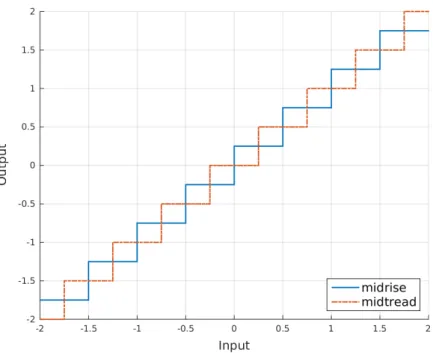
4.3.2 Uniform and Nonuniform Quantizers . . . 45
4.3.3 Vector Quantization . . . 46 4.4 Predictive Coding . . . 47 4.4.1 DPCM . . . 49 4.4.2 CALIC . . . 49 4.5 Transform Coding . . . 50 4.5.1 Karhunen-Loève Transform . . . 51
4.5.2 Discrete Cosine Transform . . . 52
4.5.3 Subband Coding . . . 53
4.5.4 Discrete Wavelet Transform . . . 54
4.5.5 Bitplane and Significance-Map Coding . . . 56
4.5.6 Set Partitioning in Hierarchical Trees . . . 56
4.5.7 3D Wavelet Based Compression of Hyperspectral Images . . . 59
4.6 JPEG 2000 . . . 60
4.6.1 Pre-Processing . . . 61
4.6.2 DWT . . . 61
4.6.3 Quantization . . . 62
4.6.4 Entropy Coding . . . 63
4.6.5 Bit Stream Organization . . . 64
4.7 CCSDS Recommendation for Data Compression . . . 64
4.7.1 CCSDS-122. . . 65
4.7.2 CCSDS-123. . . 65
4.8 Summary . . . 65
5 Sparse Representation Based Lossy Hyperspectral Image Compression 67 5.1 Introduction . . . 67
5.2 Background and Related Work . . . 68
5.2.1 Dictionary Learning . . . 68
5.2.2 Related Work . . . 69
5.3 Sparse Representation Based Hyperspectral Image Compression . . . 71 v
5.3.1 Dictionary Training . . . 71
5.3.1.1 Multiscale Spatial Spectral Dictionary Learning . . . 73
5.3.1.2 Dictionary Atom Sorting . . . 74
5.3.2 Hyperspectral Image Compression . . . 75
5.3.3 Decompression . . . 80
5.4 Experiments . . . 80
5.4.1 Experimental Data Sets. . . 80
5.4.2 Experiment Setup. . . 82
5.4.3 Results of Experiments and Discussion . . . 83
5.4.3.1 Compression Performance. . . 83
5.4.3.2 The Comparison of Base and Updated Dictionaries. . . 86
5.4.3.3 Tuning Dictionary Learning Parameters. . . 87
5.4.3.4 The Drawbacks of the Proposed Method . . . 88
5.5 Conclusion . . . 89
6 Sparse Representation Based Hyperspectral Image Classification 93 6.1 Introduction . . . 93
6.2 Related Work . . . 95
6.2.1 SVM Classification Approach . . . 95
6.2.1.1 SVM Formulation . . . 95
6.2.1.2 SVMs for Hyperspectral Image Classification. . . 97
6.2.2 Sparse Representation Based Classification Approach . . . 98
6.2.3 KNN Classification Approach . . . 99
6.3 The Proposed Sparse Representation Based Classifiers . . . 100
6.3.1 Dictionary Training . . . 100
6.3.2 Hyperspectral Image Classification Using Contextual Sparse Coefficients 101 6.4 Experiments . . . 102
6.4.1 Data Set Description . . . 102
6.4.2 Experiment Design . . . 104
6.4.3 Experimental Results . . . 105
6.4.3.1 Classification Results of Various Approaches . . . 105
6.4.3.2 Classification Performance on Varying Parameters for the Pro-posed Methods. . . 107 6.5 Conclusion . . . 109 7 Conclusion 115 7.1 Summary . . . 115 7.2 Future Work . . . 116 7.3 Conclusion . . . 116 Bibliography 119 vi
List of Figures
2.1 The Concept of Imaging Spectroscopy . . . 10
2.2 The 3D Structure of Hyperspectral Cube . . . 11
2.3 Reflectance Spectra of Soil, Green and Dry Vegetations . . . 11
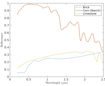
2.4 Reflectance Spectra of Brick, Starch (Corn) and Limestone . . . 12
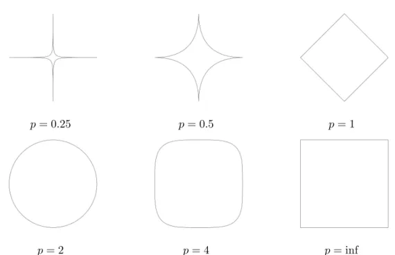
3.1 The Behaviour of|α|pfor Different Values ofp . . . . 22
3.2 Comparison Among Different Balls of Sparsity Inducing Norms . . . 23
3.3 The Intersection Between`p-ball and the SetDα=x. . . 23
3.4 Examples of Regularization Path . . . 28
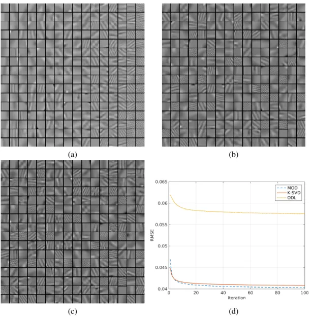
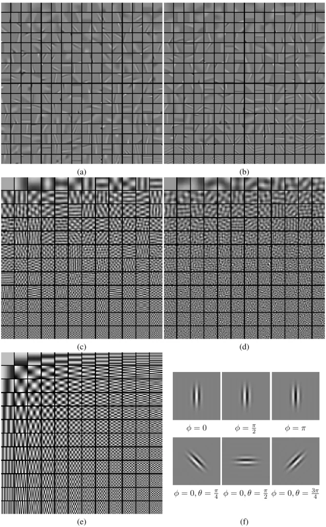
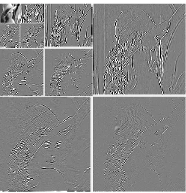
3.5 Visual Comparison of Dictionaries for Image Data . . . 35
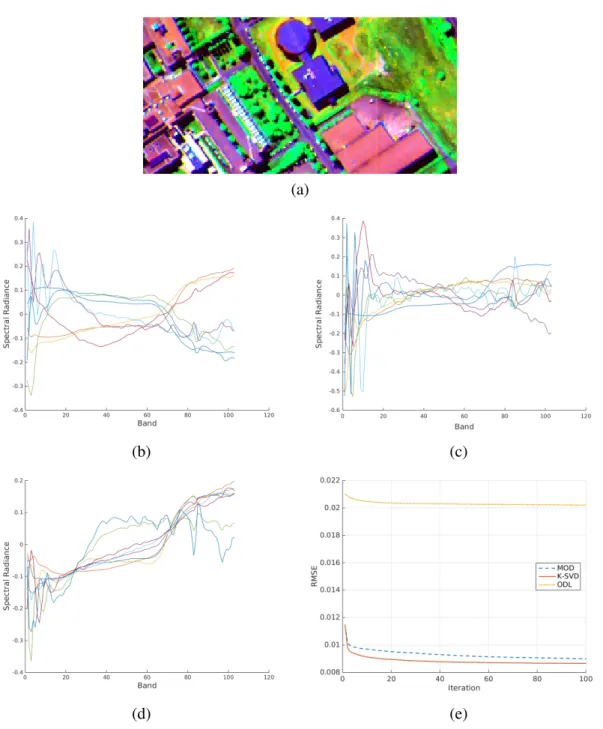
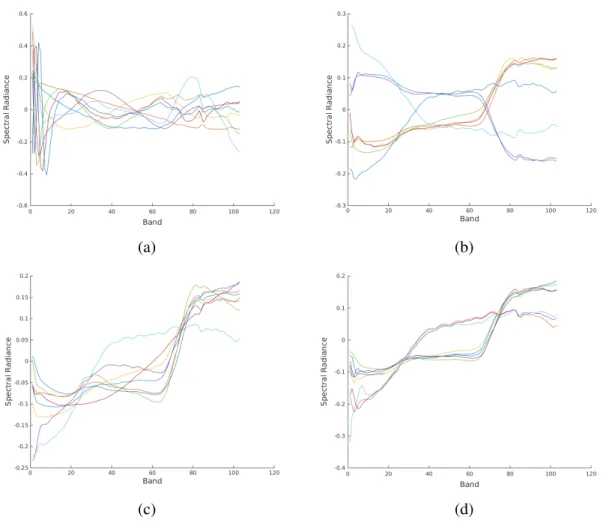
3.6 Visual Comparison of Dictionaries for A Hyperspectral Image . . . 37
3.7 Visual Comparison of Principle Components and Dictionaries for A Hyperspec-tral Image . . . 38
3.8 Dictionary Visualization . . . 39
4.1 Input-Output Mappings for Two Scalar Quantizers . . . 45
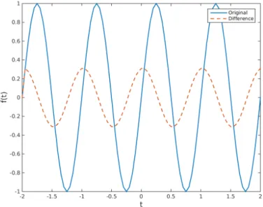
4.2 The Comparison of Dynamic Ranges of the Outputs of an Original and Its Pre-dictive Sequences . . . 48
4.3 The Architecture of a Basic Transform Coding . . . 51
4.4 One-Dimensional, 3-Level Wavelet Decomposition . . . 54
4.5 Two-Dimensional, 2-Level Wavelet Decomposition . . . 55
4.7 A Ten-Band Wavelet Decomposition . . . 57
4.8 The Spatial Orientation Tree for the Dyadic Wavelet Decomposition . . . 58
5.1 The Proposed Hyperspectral Image Lossy Compression Framework based on Dic-tionary and Sparse coding. . . 72
5.2 Illustrative Examples of Sparse Coefficients, Dictionary Atoms, Original and Re-constructed Hyperspectral Image Pixels . . . 76
5.3 The Process of Hyperspectral Image Compression using Dictionary and Sparse Coding. . . 77
5.4 Grayscale Images of Group 1 Data Sets . . . 81
5.5 False Colour Images of Group 2 Data Sets . . . 81
5.6 Grayscale Images of Group 3 Data Sets . . . 91
5.7 Rate-Distortion Curves for the Compression of Sub-Cubes from Lunar Lake and Moffett Field II Data Sets using Different Dictionary Sizes . . . 92
5.8 Rate-Distortion Curves for the Compression of Sub-Cubes from Bay Area I Using Various Values ofµ . . . 92
6.1 The diagram of the proposed classification framework.X– the HSI data after pre-processing;D– the dictionary;A– the matrix consists of the sparse coefficients;
CSC– contextual sparse coefficients; . . . 100
6.2 Classification Maps for Indian Pines Data Set . . . 108
6.3 The Classification Performance of CSCSVM for Indian Pines Data Set using Var-ious Regularization Parameters . . . 111
6.4 The Classification Performance of CSCNN for Indian Pines Data Set using Vari-ous Regularization Parameters . . . 112
6.5 The Selected Class Accuracies of CSCSVM for Indian Pines Data Set using Dif-ferent Regularization Parameters . . . 113
6.6 The Classification Performance of CSCSVM for Indian Pines Data Set using Var-ious Dictionary Sizes . . . 114
List of Tables
4.1 Decoder Mappings . . . 455.1 Coefficients for 5/3 Filter Bank . . . 74
5.2 Coefficients for 9/7 Filter Bank . . . 74
5.3 Compression Performance of Various Methods for Group 1 Data Sets . . . 84
5.4 Compression Performance of MSSD with or without the Dictionaries Being Trans-mitted . . . 85
5.5 Compression Performance of Various Methods for Group 3 Data Sets . . . 86
5.6 Compression Performance of Various Methods for Group 2 Data Sets . . . 87
5.7 Performance Comparison of the Base and Updated Dictionaries. . . 87
5.8 Bit Allocation for Various Components using SRSD. . . 88
5.9 Sparse Coding Performance for 3 Selected Data Sets using SRSD. . . 89
6.1 The Ground Truth Classes in AVIRIS Indian Pines Data Set. . . 103
6.2 The Ground Truth Classes in ROSIS University of Pavia Data Set. . . 103
6.3 The Ground Truth Classes in AVIRIS Salinas Data Set . . . 104
6.4 Classification Performance for Indian Pines Data Set . . . 105
6.5 Classification Performance for University of Pavia Data Set . . . 106
6.6 Classification Performance for Salinas Data Set . . . 107
6.7 The Running Time for Dictionary Training using Variousλs . . . 109
List of Algorithms
1 Matching Pursuit Algorithm . . . 25
2 Orthogonal Matching Pursuit Algorithm. . . 26
3 The Method of Optimal Directions Algorithm. . . 31
4 The K-SVD Algorithm . . . 32
5 Online Dictionary Learning . . . 33
6 Dictionary Update . . . 34
7 Huffman Decoding . . . 43
8 Encoding the Sparse Representation Matrix . . . 77
9 A Uniform Scalar Quantizer . . . 78
Acronyms
1D One-dimensional
2D Two-dimensional
3D Three-dimensional
ADPCM Adaptive DPCM
AVIRIS Airborne visible/infrared imaging spectrometer
BP Basis pursuit
BPE Bit plane encoder
CALIC Context-based adaptive lossless image codec CCSDS Consultative committee for space data systems CFAR Constant false-alarm rate
DCT Discrete cosine transform
DPCM Differential pulse code modulation DWT Discrete wavelet transform
EBCOT Embedded block coding with optimised truncation EZW Embedded zerotree wavelet
GAP Gradient-adjusted prediction GLA Generalised Lloyd algorithm HSI Hyperspectral image
ICT Irreversible colour transform IDC Image data compression
JPEG Joint photographic experts group KLT Karhunen-Loève transform
M-NVQ Mean-normalized vector quantization
MP Matching pursuit
MSB Most significant bit MSE Mean squared error
MSSD Multi-scale spectral dictionary
NN Nearest neighbour
ODL Online dictionary learning OMP Orthogonal matching pursuit PCA Principle component analysis PDF Probability density function PPI Pixel purity index
PSNR Peak signal to noise ratio RCT Reversible colour transform RMSE Root mean squared error SAM Spectral angle mapper
SD Spectral dictionary SKA Square kilometre array SNR Signal to noise ratio
SPECK Set partitioned embedded block SPIHT Set partitioning in hierarchical trees SRSD Sparse representation spectral dictionary SVD Singular value decomposition
SVM Support vector machine VQ Vector quantization
Chapter 1
Introduction
In signal and image processing, finding an appropriate model for the data is the heart of the problem. Sparsity based models, or simply sparsity models, have been widely adopted as the choice of models in this topic. Using sparsity models, many types of signals such as still image, video and acoustic can be sparsely represented through linear transforms. These models assume that the signal or image vectors, usually lie in a combination of subspaces, where each subspace is spanned by a few elements from a set of basis vectors. Sparsity models have received signif-icant attention in image processing in a variety of applications, including image compression, denoising, classification, to name a few. The well known digital image coding standard joint pho-tographic experts group (JPEG), and its successor JPEG 2000 are both based on transforms that lead to sparsity.
A commonly adopted transform coding strategy is to apply a linear transform to an image vec-torx∈RMby taking the multiplication of the image with a set ofbasis vectors{w1,w2, . . . ,wL},
wherewi ∈RM. We may express this transform in vector notation as
b=WTx, (1.1)
where the columns in matrixWcorrespond to the basis vectors. The goal in such a transform coding is to find a set of orthogonal basis vectors that span the vector space of input images. The coefficient vectors obtained under these basis vectors usually lead to some criterion of optimality, such as decorrelation and sparseness. Discrete cosine transform (DCT) is an example of such transform coding strategy.
An alternative way of transforming images within the linear framework is using a generative sparsity model introduced byOlshausen and Field[1997]. It is based on learning a dictionaryD
using a set of training data. The learnt dictionary is utilizedchecks for sparsely representing the input images or signals. This type of sparsity models are often referred to assparse representation
in the literature.
An imagex, using sparse representation, is modelled in terms of the linear superposition of a set of vectors{d1,d2, . . . ,dK}, commonly termed asatoms.
x=Dα, (1.2)
where the atoms inDcorrespond to a set of learned vectors, andα∈RKis the coefficient vector. In contrast to the transform in (1.1), the vectors in dictionaryDare not necessarily orthogonal to each other, and it requires custom algorithms for finding the coefficient vectorα. Specifically, if the dictionaryDis overcomplete, which is true when the number of atoms inDexceeds the dimensionality of the input vector, then the solution forαis not unique.
1.1 Problem Motivation 2
An image is always associated with a set of data and visually interpretative entities. The data set associated with an image can be understood as an array with each entry being an intensity value and referred to as a pixel. A typical colour image has three channels (or bands) and each of them conveys information at different electromagnetic wavelengths. In fact, the human visual system needs only three wavelength channels, i.e., red, green, and blue (RGB), to see colours [Geladi
et al. 2007]. However, there are many imaging techniques that are able to acquire more than
three bands, and this number is constantly growing. Hyperspectral imaging is one among such techniques. It is a spectral imaging modality that obtains environmental and geographical infor-mation by imaging ground locations from airborne or spaceborne platforms. It is also frequently applied in laboratories and hospitals. Hyperspectral imaging typically uses hundreds of contigu-ous spectral bands that are regularly spaced from infrared to ultraviolet spectrum. For example, the airborne visible/infrared imaging spectrometer (AVIRIS) delivers calibrated images of the upwelling spectral radiance in 224 contiguous spectral bands with wavelengths from0.4µm to
2.5µm [NASA JPL 2015]. The image data results from hyperspectral imaging is viewed as a
three-dimensional (3D) data cube.
1.1 Problem Motivation
Modern hyperspectral sensors have high spectral resolutions covering up to several hundred bands. The transmission and storage of the resultant large volume of data collected by such sensors mean that data compression is an essential feature of the systems incorporating hyperspectral sensors. Hyperspectral data compression has received particular interest in hyperspectral image process-ing and analysis due to several reasons. Firstly, the volume of such data is commonly enormous. Secondly, there is a significant amount of redundancy in the spectral domain. Thus, by designing efficient compression schemes, high compression ratio can be achieved without loss of signifi-cant information. Thirdly, although a hyperspectral image can be viewed as a 3D image cube, it does not necessarily lead to an efficient compression technique by simply extending the existing two-dimensional (2D) image compression methods. For 2D image compression, exploiting the 2D spatial redundancy is the key. When it comes to 3D hyperspectral image cube, the spectral domain often demands distinctive approaches in reducing the redundancy than those for spatial domain. Lastly, the compression performance of hyperspectral data is evaluated not only in terms of compression ratio, but also information preserving. In fact, the latter is often more important than the former. Unlike the conventional images with high spatial resolutions, hyperspectral im-ages have relatively lower spatial resolutions. A pixel in a hyperspectral image may have mixed spectra. It is crucial to preserve such information in data compression for further data analysis in various applications, such as target detection and anomaly detection. For this purpose, spec-tral compression and spatial compression should be decoupled [Chang 2013]. One might argue that lossless compression should be preferred over the lossy one for the purpose of information preserving. However, lossless compression only allows very limited compression ratios, and the abundant spectral and spatial redundancies in hyperspectral image can not be adequately reduced. As a result, storage and bandwidth could be wasted.
Compression of still images has been a very active research and application field. It offers many contributions in the literature, and a number of standard image compression schemes exist. A representative standard would be the JPEG 2000, which is a general purpose, wavelet transform based compression framework. By general purpose, we mean that the standard does not
neces-3 1.2 Problem Statement and Research Objectives
sarily adapt to or perform optimally for some specific families of images, including hyperspectral images. It is often necessary for different compression algorithms to be developed for specific types of images. Previous investigations of hyperspectral data compression include differential pulse code modulation (DPCM) or predictive coding based methods [Roger and Cavenor 1996;
Wu and Memon 1997], vector quantization (VQ) based methods [Kaukoranta et al. 1999;Qian
2004;Rizzo et al. 2005], and transform coding based methods [Goyal 2001;Penna et al. 2007]. Transform coding plays an important role in hyperspectral image compression. DCT and dis-crete wavelet transform (DWT) have been applied successfully in still image compression stan-dards JPEG and JPEG 2000, respectively. Both DCT and DWT offer excellent energy compaction features, which are essential in data compression, in these standards. On the other hand, given a dictionary, an image can be approximated as a linear combination of very few dictionary atoms. That is, in sparse representation domain, the coefficient is sparse and hence, displays energy com-paction feature. A natural question is if sparse representation can be applied in data compression. This leads to the primary research question of this thesis.
Recent work on various image processing applications show that sparse representation based methods could lead to state-of-the-art results. These include but not limited to vision tasks such as image classification [Bahrampour et al. 2016], image denoising, deblurring, inpainting [Elad and Aharon 2006;Elad et al. 2010], image restoration [Mairal et al. 2008a]. There are also recent works on applying sparse representation to process some specific types of images, such as facial image [Bryt and Elad 2008], video [Guha and Ward 2012] and medical imaging [Li et al. 2012]. In addition, the application of sparse representation has been widely extended to hyperspectral im-age processing tasks such as classification [Chen et al. 2011a;Soltani-Farani et al. 2013], target detection [Chen et al. 2011b], denoising [Zhao and Yang 2015;Lu et al. 2016], anomaly detec-tion [Xu et al. 2016], and hyperspectral unmixing [Iordache et al. 2011 2014]. Compared with these, there is relatively little work on applying sparse representation to data compression, and in particular hyperspectral data compression.
Motivated by the recent advances in theoretical, methodological, application aspects of sparse representation, in this thesis, we present an application of sparse representation in the lossy hyper-spectral image compression framework. The study is extended further to investigate hyperhyper-spectral image classification using sparse representation.
The study in this thesis is not only relevant to hyperspectral imagery, it certainly contributes to the broader communities of data compression, image and signal processing. For instance, they could be the ones in the exciting square kilometre array (SKA) project [SKA 2015]. The SKA project is an international effort to build the world’s largest radio telescope. It aims at enabling astronomers to monitor the sky in unprecedented detail and survey the entire sky thousands of times faster than any systems currently in existence [SKA SA 2015]. Signal and image processing is an integral part in the SKA project to produce high resolution radio images and to analyse them. The central data processing elements in the SKA project will need to process and transmit the data received by thousands of telescopes. The input data rates are expected to be in the hundreds of gigabits per second and need to be processed in soft-realtime. One of the main challenges in this scenario will be the development and deployment of sophisticated radio frequency interference mitigation, calibration and imaging algorithms. The current sparsity based models, including the sparse representation, adapted to the high dimensional data such as hyperspectral imagery would provide substantial insights to the relevant tasks in SKA project.
1.3 Overview of Methodology 4
1.2 Problem Statement and Research Objectives
The primary research questions in this thesis are:1. How sparse representation can be effectively utilized in hyperspectral image compression framework?
2. If sparse representation is employed in the hyperspectral image compression, are the sparse coefficients of hyperpsectral image pixels applicable in the subsequent hyperspectral image processing tasks, such as classification?
Problem Statement:Based on the research questions above, the problem to be addressed in this thesis concernsthe applications of sparse representation to i) hyperspectral image compression, and ii) hyperspectral image classification.
The aim of this thesis is to effectively apply sparse representation to hyperspectral image compression and hyperspectral image classification. We set the specific research objectives as follows.
1. Development of a hyperspectral image compression framework that deploys sparse repre-sentation.
2. Implementation of a prototype of the proposed compression framework.
3. Dictionary learning for effective exploitation of the spectral and spatial correlations in a hyperspectral image.
4. Evaluation and comparison of the proposed compression method to the existing state-of-the-art hyperspectral image compression approaches, which include JPEG 2000 standard. 5. Development and implementation of a hyperspectral image classification scheme that
in-corporates sparse representation.
6. Evaluation and comparison of the proposed classification approach to other representative hyperspectral image classification methods including sparse representation based ones. A number of problems may be subsumed under the primary problems. These include:
• A dictionary is a key element in sparse representation. How do we alleviate the overhead of transmitting the dictionary in a data compression framework?
• When we pursue reducing the data size in lossy data compression, it is also important to preserve information. How do we achieve this goal in sparse representation based compres-sion scheme?
1.3 Overview of Methodology
In this section, we give an overview of our methodology for applying the sparse representation to hyperspectral image compression and classification. The proposed lossy hyperspectral image compression framework consists of two integral parts: encoder and decoder. Sparse representa-tion is employed in the encoder in two aspects, that is dicrepresenta-tionary learning and sparse coding.
Dictionary Learning: Dictionaries are learned to exploit the redundancy of a hyperspectral image in spectral domain, and such a dictionary is termed as spectral dictionary (SD). Online dictionary learning algorithm [Mairal et al. 2008a] is applied for the training process. Online dictionary learning is a stochastic gradient descent based approach that picks a random training
5 1.4 Contribution of The Thesis
sample at each iteration and updates the objective function on the basis of this example only. It optimizes the expected cost of the objective function rather than the empirical cost. Airborne or spaceborne hyperspectral images are often obtained over the same or similar geological locations. This makes it possible to learn a base dictionary offline. By ‘offline’ we mean the dictionary learning process is not included as a part in the encoder. The base dictionary can be used in the sparse representation of hyperspectral images from the similar geological locations. To improve upon the representative capacity of the base dictionary, a dictionary update step is included in the encoder. This approach has two advantages. One is to improve the adaptivity of the dictionary with moderate computational cost. The other is reducing the cost of transmitting the dictionary, as we only need to transmit the difference between the base and updated dictionaries.
The spectral dictionaries discussed above can only be utilized for exploiting the spectral re-dundancy in hyperspectral images. In order to exploit the spatial rere-dundancy as well, we take an approach where the dictionaries are trained in the multi-scale spectral domain, and such a dic-tionary is termed as MSSD. Specifically, the DWT is performed in the spatial domain to exploit the spatial redundancy in hyperspectral images. This is followed by training multi-scale spectral dictionaries in the resulting wavelet spectral domain.
Sparse coding:Using a learned dictionary and sparse coding, the hyperspectral image pixels are transformed into sparse coefficients. Being the main information to be transmitted to the decoder, these sparse coefficients are represented as a sparse matrix. Subsequently, an efficient representation of a sparse matrix, called index-value pair, is applied. The index-value pairs of the sparse coefficients have two types of information, one is position index, and the other is coefficient value. As such, these are treated in separate manners in the encoding stage.
Besides the sparse coefficients, the dictionary and the mean values of the hyperspectral image pixels, also need to be transmitted. The information with non-integer values are quantized using uniform scalar quantizers. Huffman coding is applied in the entropy coding to formulate the final bit stream.
The hyperspectral image classification in this thesis is a supervised classification approach that utilizes sparse representation. The proposed method starts with learning a dictionary that induces sparsity in the representation coefficients and minimizes the reconstruction error. In order to incorporate the contextual information into the spectral sparse coefficients, we enforce smooth variations in the neighbourhoods of pixels by applying a local filter on sparse coefficients. These contextual sparse coefficients are then used as feature vectors for two popular classifiers, namely SVMs and nearest neighbour (NN) classifier, for their robustness and simplicity.
A highlight of the methodology in this thesis is that the proposed compression and classifica-tion approaches are evaluated not only in terms of relevant performance criteria that are commonly used in the literature, but also are compared to some of the state-of-the-art hyperspectral image compression or classification methods.
1.4 Contribution of The Thesis
The successful applications and developments of sparse representation in various signal and im-age processing tasks, including hyperspectral imim-age (or data) processing, show the effectiveness of this particular sparsity based model. In contrast, there is little work done in respect of the ap-plication of sparse representation to data compression. Theoretically, however, due to its sparsity inducing nature, sparse representation is suitable to be applied in data compression. This thesis is
1.6 Organisation of The Thesis 6
such an attempt to incorporate sparse representation with hyperspectral image compression. The experimental results show that the proposed approach is comparable to some of the state-of-the-art hyperspectral image compression methods. This shows that sparse representation is indeed a very effective method to exploit the spectral redundancy in hyperspectral images.
The sparse representation based hyperspectral image classification approach reveals the ef-fectiveness of sparse coefficients in the discriminative tasks such as classification. While the work in this regard takes mostly standard approaches, it presents a much simpler way of applying sparse representation to the concerned task and achieves similar or better results. In particular, the dictionary learning and sparse coding may take the same approach in both the compression and classification of hyperspectral images. Under such scenario, it becomes feasible in the proposed hyperspectral image compression framework that the side information, including the dictionary, can be entirely excluded in the final bit stream. Thus, the major challenge of transmitting the dictionary can be alleviated.
So far, some of the results of this thesis are either published or accepted for publication. They are included in the following list.
1. H. Wang and T. Celik, “Sparse representation based lossy hyperspectral data compression,”
2016 IEEE International Geoscience and Remote Sensing Symposium (IGARSS),pp. 2761-2764, July 2016, Beijing, China.
2. H. Wang and T. Celik, “Sparse representation based hyperspectral data processing: lossy compression,” IEEE Journal of Selected Topics in Applied Earth and Remote Sensing,
10(5), pp. 2036-2045, May 2017.
3. H. Wang and T. Celik, “Sparse representation based hyperspectral image classification,”
Signal, Image and Video Processing(2018). https://doi.org/10.1007/s11760-018-1249-1.
1.5 Notation
In This Thesis , constant scalar values are denoted by upper-case letters, and variables by lower-case ones. Vectors are denoted by bold lower-lower-case letters, and matrices by bold upper-lower-case ones.
1.6 Organisation of The Thesis
The rest of this thesis is organised as follows. Chapter2gives an overview of some of the prin-ciples of hyperspectral imaging sensors, the methods of data acquisition, and the characteristics of the data acquired. It also gives a brief discussion of some common tasks and approaches in hyperspectral image processing.
Chapter3presents a review of sparse representation, where its theoretical background, rele-vant existing algorithms for dictionary learning and sparse coding are studied.
The general topics of data compression are discussed in Chapter4, with the focus on hyper-spectral image compression. These include entropy coding, predictive coding, quantization, and transform coding. Brief overviews of popular hyperspectral image compression methods, as well as the latest image compression standards from JPEG and consultative committee for space data systems (CCSDS) are also included in this chapter.
Chapter5provides the details of the proposed lossy hyperspectral image compression frame-work based on sparse representation. It also discusses some related frame-work in data compression
7 1.6 Organisation of The Thesis
based on sparse representation. Further, it presents the evaluation of the proposed method includ-ing the experimental setup, results, and discussions.
Chapter6introduces the proposed sparse representation based hyperspectral image classifi-cation method. It includes the details of related work in this topic, the evaluation and comparison results of various hyperspectral image classification methods, and the related discussions.
Finally, Chapter7concludes this thesis and proposes some possible future work.
Note that efforts are taken to write each chapter independently, in the hope that they are self contained. Thus, minor repetitions of some contents are present in Chapters3,5, and6.
Chapter 2
Hyperspectral Imaging
Remote sensing of the Earth provides a vital form of information not easily acquired by con-ventional surface observation. The advances in aviation and space exploration inevitably lead to the integration of these technologies with remote sensing. Imaging spectroscopy, a major tech-nique for remote sensing, is capable of acquiring images in contiguous, dozens or hundreds of spectral bands throughout the visible and solar-infrared intervals of the electromagnetic spec-trum. The resulting image data sets are referred to ashyperspectral imageryor simply hyperspec-tral image. Hyperspectral imagery characterizes the reflection of light against objects. It uses the fundamental principles of the interrelations among colour, frequency and wavelength of nat-ural light [Borengasser et al. 2007]. Multispectral imagery, on the other hand, usually contains a small number of relatively broad wavelength spectral bands [Borengasser et al. 2007;Chang 2007b]. In addition, multispectral imaging systems often have their spectral bands widely irreg-ularly spaced, while hyperspectral imaging systems have spectral bands that are adjacent to each other and regularly spaced.
Remote sensors allow us a vantage point to obtain not only vertical views of the Earth’s land surface, but also information covering large areas quickly. This raises the question of dealing with large volumes of data, even with relatively low spatial resolutions of remote sensing data. Higher spatial resolution results in larger quantities of data, more sophisticated sensors and con-trol systems, increased requirements for storage and downlink bandwidth. These motivated the consideration of ways to collect information via spaceborne or airborne platforms from image data with lower spatial resolutions. This resulted in the concept of using spectral measurements of a pixel to analyse the type of ground cover a pixel represents, instead of using spatial variations and the conventional image processing techniques that rely on higher spatial resolution [Landgrebe 1999].
Hyperspectral imaging spectrometers are capable of capturing images that contain both spa-tial and spectral information at relatively fine resolutions. The resulting data was shown to be useful in identifying different materials, and producing thematic maps that display the spatial distribution of these materials. This property led to broad applications of hyperspectral imaging in different problems, adapting the processing used to extract relevant information. In remote sensing, the applications of hyperspectral imaging cover a variety of fields such as land use moni-toring [Bachmann et al. 2002], agriculture [Haboudane et al. 2004], urban mapping [Benediktsson et al. 2003 2005], coastal environment and water monitoring [Corson et al. 2008], geology [Kruse et al. 2003], mine detection [Zare et al. 2008], chemical agent detection [Kwan et al. 2006], and others [Meer and de Jong 2001;Eismann et al. 2009;Nasrabadi 2014, and references therein]. In general, these applications perform the tasks of detection, recognition, or classification of anoma-lies or targets, or characterization of background scenes. Beyond remote sensing, hyperspectral
9 2.1 Imaging Spectroscopy
imaging has also found applications in various fields such as pharmaceuticals [Ravn et al. 2008], medical [Harvey et al. 2002], and food quality and safety [Elmasry et al. 2012].
Hyperspectral images contain a wealth of information. Processing and analysing this type of data, such as information extraction, requires an understanding of what properties of land surface materials are captured and how they are measured by hyperspectral sensors. For this purpose, in the following section, we investigate briefly some of the principles of hyperspectral imaging sensors, methods of data acquisition and the characteristics of the data acquired. We also discuss some common tasks and approaches in hyperspectral image processing before we summarize this chapter.
2.1 Imaging Spectroscopy
Spectroscopyis the study of light as a function of wavelength that has been emitted, reflected, or scattered from a solid, liquid, or gas [Clark 1999]. As photons enter a material, reflection, trans-mission and absorption all occur. Material surfaces are also capable of emitting photons under certain conditions. The varying characteristics of photon absorption, reflection or emission from different materials provide us with information about the materials. When applied to the optical remote sensing, spectroscopy deals with the spectrum of sunlight that is absorbed, reflected or scattered by materials on the Earth’s surface. Based on spectroscopy, instruments called spec-trometersare developed to measure the light energy reflected from a test material. An optical refraction device such as a prism in a spectrometer splits the light into many narrow, consecutive wavelength bands. The energy in each one of these bands is measured by a separate detector. By using hundreds or thousands of detectors, spectrometers can make spectral measurements of bands as narrow as several nanometres.
As a type of remote sensing instrument, imaging spectrometers are passive sensors. Passive sensors detect natural energy that is emitted or reflected by the objects they observe. Reflected sunlight is the most common source of radiation measured by passive sensors. On the other hand, active sensors provide their own source of energy to illuminate the objects. They emit radiation towards the targets, and then detect and measure the reflected or backscattered radiation from them [NASA 2018].
Imaging spectroscopy is a technique for obtaining a spectrum at each position of a large array of spatial positions, so that any one spectral wavelength can be used to make a recognizable im-age [Clark 1999]. In remote sensing literature, imaging spectroscopy is also known asimaging spectrometry, hypespectral imaging, or ultraspectral imaging. The concept of imaging spec-troscopy in the case of satellite remote sensing is illustrated in Figure2.1.
Hyperspectral images are produced byimaging spectrometers. Most imaging spectrometers used are aboard air- or space-based platforms. For example, the NASA’s AVIRIS is flown on the ER-2 jet at 20km above the ground. These imaging spectrometers are developed to measure spectra as images in some or all of the 400− 2500 nm electromagnetic spectral region. As the analysis of hyperspectral data in this part of the spectrum mainly deals with the reflectance nature of solid and liquid materials. These hyperspectral images are typically arranged as a 3-dimensional data cube as shown at the centre of Figure2.2. Hyperspectral data can be viewed as a set ofpixel vectors, each consists of a group of spectral components for the same spatial location. Each component of a pixel vector corresponds to the received energy at a particular wavelength. The spectra of a hyperspectral pixel vector is shown at the left of Figure2.2. Alternatively, we
2.1 Imaging Spectroscopy 10
Figure 2.1: The concept of imaging spectroscopy (Source: [Shaw and Burke 2003]). An airborne or space-borne sensor samples multiple spectral wavelengths over a ground based scene. In the resulting image, each pixel contains a spectral measurement of reflectance. The spectral variance of three types of materials is also shown in the graph.
can view the hyperspectral data cube as being composed of a group of co-registered 2D images with each of them corresponding to a particular wavelength. These images are often referred to asband imagesor simplybands. An example band image is shown at the right of Figure2.2.
2.1.1 Reflectance and Radiance
Through imaging spectroscopy, we want to obtain a measurement, called spectral reflectance, which reveals the property of a particular material. Reflectance is the ratio of the amount of energy leaving a target to the amount of energy striking the target. It is a fractional number between 0 and 1. Reflectance varies with wavelength for most materials because light at a certain wavelength is reflected, scattered or absorbed differently. Figures2.3and2.4show the spectra of different materials. The former figure shows three common Earth surface materials, namely green vegetation, dry vegetation, and soil, and the latter shows the spectra of three materials, namely, bricks, starch (corn), and limestone. Each spectral curve shows the differing levels of absorption of light energy of the corresponding material. For example, vegetation has higher reflectance (or lower absorption) in the near infrared range, and lower reflectance of red light than soil. In the case of green and dry vegetations, the spectral curves are generally similar due to the two materials are made of the same basic components. The shape of the spectral curve, the position and strength
11 2.1 Imaging Spectroscopy
Figure 2.2: The 3D structure of hyperspectral cube (Source: [Manolakis et al. 2003]).
of absorption bands are often used in distinguishing among different surface materials.
Figure 2.3: Reflectance spectra of Soil, Green and Dry vegetations (Source: [Clark 1999]).
Radiancetypically describes the amount of light the imaging spectrometer detects from the object being observed. This is the quantity directly measured by a spectrometer. Radiance indi-cates how much of energy emitted or reflected from a surface is received by an imaging spectrom-eter looking at the target at a certain angle. While radiance reflects the total amount of emission or reflectance,spectral radiance indicates the amount of radiance at a single wavelength. Ra-diance data contains information relevant to the material composition of each pixel. However, this information is generally perturbed in the collected data by various aspects. These include environmental factors such as weather, solar illumination, downward and upward atmospheric passages, and adjacency effects, as well as sensor characteristic influences. These factors need to be compensated effectively through the combination of sensor calibration [Green et al. 1990] and atmosphere normalization [Green et al. 1993]. Several commonly used strategies for converting AVIRIS radiance data to reflectance data is discussed in [Farrand et al. 1994].
2.1 Imaging Spectroscopy 12
Figure 2.4: Reflectance spectra of brick, starch (corn) and limestone.
2.1.2 Sensors
The critical part of hyperspectral imaging is the sensor. The imaging process in hyperspectral sensing involves the focusing of light from a small region of the Earth’s surface to a given detector unit that forms a pixel in the resulting image [Chang 2007a]. The spatial resolution of the image is determined by the sizes of relevant hardware elements such as the detector and lens. The sensors form an image by arranging the pixels in two-dimensional array. Each pixel has a number of spectral components. Thus, a hyperspectral image is often described as a data cube. The two spatial dimensions include along-track dimension (column) and its orthogonal dimension (row or scan line) which is sometimes referred to asswath. The along-track dimension is built up by the motion of the platform carrying the sensor, and the swath is the width of the field-of-view covered by the sensor. The spectral dimension consists of a number of spectra at varying wavelengths (see Figure2.1).
Modern imaging spectrometers differ in the methods they collect data. These methods focus on two primary aspects, namely, spatial scanning and spectral selection. From the spatial point of view, there are a number of basic ways the sensors form (2D) images. For different approaches, the focal plane complexity and platform stability requirements differ for the sensors [Schaepman 2009;Chang 2007a]. In the following, we briefly describe the three approaches for spatial scan-ning. In general, whiskbroom imaging spectrometer collects series of pixels, pushbroom scanners series of lines, and filter wheel cameras series of monochromatic images.
Whiskbroom scannerscover the field-of-view by a mechanized angular movement of a scanning mirror sweeping from one edge of the swath to the other, or by the mechanical rotation of the sensor. The scanner view of the field at a moment is a single spatial pixel and its associated
13 2.2 Hyperspectral Image Processing
spectral components. The image lines are collected using an across-track scanning and the entire image is obtained using the forward movement of the carrier platform.
Pushbroom scannersacquire a series of one-dimensional samples orthogonal to the platform line of flight, with along-track spatial dimension constructed by the forward movement of the platform. The spectral component is obtained by dispersing the incoming radiation onto an area array. This type of scanners do not require the use of moving mirror because a linear array of detectors image a line of image across the field of view simultaneously.
Filter wheel camerasare opto-mechanical sensors that change the spectral sensitivity of various channels using a turnable filter wheel in the optical path. Such a camera relies on the use of two-dimensional detector array in the focal plane to acquire a monochromatic frame of the field-of-view at one time. The spectral components are obtained by rotating the filter wheel to different band pass filters.
On the other hand, the spectral measurements are accomplished by several techniques includ-ingprism,grating,filter wheel,interferometer, andacousto-optical tunable filterorliquid crystal tunable filter. Using prism, the incident light is diffracted in different directions, depending on the wavelength. The linear detectors are then positioned at appropriate locations to the prism to sam-ple the varying spectra. Grating works similar to that of prisms by dispersing the light spatially, except that the light is reflected rather than diffracted through the spectral selection elements. For filter wheel approaches, interference filters are arranged around the edge of a wheel, which are rotated in front of the detector to collect data at various wavelengths. The interferometer systems collect interferograms which must be converted to optical spectrum. Finally, the acousto-optical and liquid crystal tunable filters work on the principle of selective transmission of light through materials in which acoustic waves are passed or a varying voltage is applied [Chang 2007a].
The recent developments in hyperspectral imaging spectroscopy mostly concentrated on air-borne spectrometers covering visible to near-infrared, and shortwave-infrared range of spectra. For an example, the AVIRIS [Green et al. 1998], designed and operated by NASA’s Jet Propul-sion Laboratory in California, USA, has been used since late 1980’s in a large number of scientific experiments and field campaigns. Deployed on NASA’s ER-2 or WB-57, flying up to 20km above the ground, AVIRIS is able to collect data with 20m spatial resolution over an estimate of 11km swath. It can also be applied at lower altitude for finer ground resolution. Among the spaceborne spectromters, Hyperion, on board NASA’s Earth Observing-1 (EO-1) spacecraft, has been one of the main providers of space based hyperspectral data. To improve the amount and quality of space based hyperspectral data, the number of space borne projects are gradually increasing. The en-vironmental mapping and analysis program (EnMAP) German imaging spectroscopy mission is one such program. EnMAP is expected to become a key system in the field of spaceborne imaging spectroscopy in potential co-existence with other comparable missions around the world [Guanter et al. 2015].
2.2 Hyperspectral Image Processing
Extracting information in hyperspectral data is an important subject. Various techniques are de-veloped recently to classify, detect, identify, quantify, and characterize the features and objects using the hyperspectral images [Chang 2007a]. Although the applications of hyperspectral imag-ing cover numerous fields, some application specific tasks are dealt with commonly. One such
2.2 Hyperspectral Image Processing 14
task isdimensionality reduction. Hyperspectral sensors are designed to capture spectral infor-mation in fine resolutions so that any narrow spectral features are adequately represented. Some sensors can achieve high resolutions in spatial feature as well. As an important task, dimensional-ity reduction tries to reduce the redundancies in both spectral and spatial domains without loss of significant information. It is implemented either explicitly or implicitly in a specific application. The most widely used approaches for dimensionality reduction is the principle component analy-sis (PCA) or Karhunen-Loève transform (KLT). Other common hyperspectral image processing tasks include the following:
• Endmember extraction and spectral unmixing involves identifying the endmembers in a hyperspectral scene, and estimating the fractional abundance of each endmember in each pixel spectrum;
• Target and anomaly detection;
• Classification is a task of assigning a class label to each pixel vector in a hyperspectral image.
A comprehensive treatment of hyperspectral image processing is beyond the scope of this thesis. Interested readers are referred to the topics, including hyperspectral image endmember extraction, unmixing, detection, classification and compression, covered in [Chang 2013; Camps-Valls et al. 2012], and some recent publications on other topics such as hyperspectral image de-noising [Chen and Qian 2011;Zhao and Yang 2015], the estimation of noise in hyperspectral images [Gao et al. 2013;Mahmood et al. 2017], and hyperspectral image fusion [Yokoya et al. 2012;Akhtar et al. 2014;Wei et al. 2015]. The main focus of this thesis is hyperspectral image compression and classification, which we discuss in detail in Chapters 4,5, and6. In the fol-lowing sub-sections, we briefly describe a few selected common tasks in hyperspectral imaging applications. These includeendmember extraction,spectral unmixing,target detection. The main reason these tasks are selected is that they share closely related techniques.
2.2.1 Endmember Extraction and Hyperspectral Unmixing
A basic approach to analysing hyperspectral image is to match each pixel spectrum to one of the reference spectra in a spectral library. The approach is effective in the case where the scene of interest includes areas of pure materials that have corresponding reflectance spectra in the reference library. However, most hyperspectral scenes include pixels of mixed materials. This is possibly due to the low spatial resolutions of most hyperspectral sensors, or the mixture of distinct materials that are formed naturally. The resulting image spectrum may resemble multiple reference spectra. In general, theendmembersrepresent the pure materials present in the image, and the set of abundances at each pixel to indicate the percentage of each endmember that is present [Bioucas-Dias et al. 2012]. In hyperspectral imaging, endmember extraction is the process of selecting a group of pure signature spectra of materials that are present in the hyperspectral scene.
Many techniques are available for endmember extraction with or without the assumption of existence of pure pixels in a scene [Plaza et al. 2012, and references therein]. A popular algorithm based on the geometrical approach is the pixel purity index (PPI) [Boardman et al. 1995]. PPI projects every spectral vector toskewers, defined as a set of random vectors. The vectors that are extremes for each skewer are counted. After a certain number of repeated projections onto different skewers, the pixels with highest count scores are the purest ones. N-FINDER [Winter
15 2.2 Hyperspectral Image Processing
1999] is another widely used approach for endmember extraction. This method is based on the fact that in the spectral domain, the simplex formed by the purest pixels has the largest volume. The algorithm finds the set of pixels that define a simplex with the largest volume.
The endmembers are used to decompose each pixel’s spectrum to identify the relative frac-tional abundance of each endmember material through the process called spectral unmixing. Spectral unmixing involves decomposing a pixel spectrum into its pure component endmember spectra, and estimating the abundance of each endmember in the pixel. Many unmixing tech-niques [Keshava and Mustard 2002;Bioucas-Dias et al. 2012;Ma et al. 2014] have been devel-oped using approaches such as geometrical [Craig 1994;Boardman et al. 1995;Winter 1999], statistical [Moussaoui et al. 2008;Dobigeon et al. 2009;Bioucas-Dias and Nascimento 2012], and sparse regression based [Iordache et al. 2011 2014]. Unmixing approaches usually start with modelling the underlying physics foundation of hyperspectral imaging, and then use these models to perform the inverse operation. Two common such models are linear mixing model and non-linear mixing model. Compared to the non-linear mixing model, nonnon-linear unmixing approaches are more complex, relying on the scene parameters that are hard to obtain. Notable nonlinear un-mixing approaches include kernel-based methods [Broadwater et al. 2011], and machine learning methods [Plaza et al. 2009b]. On the other hand, the linear mixing model is well studied and has become a standard technique. It assumes that each spectral vector can be approximated by a linear combination of the endmembers weighted by their corresponding fractional abundances. That is, given a set of endmembers as the columns in matrixΦ ∈ RM×P, a spectral vectorx ∈ RM is modelled by x= P X j=1 Φjβj +, (2.1)
whereΦj ∈RM,j= 1,2,· · · , P, is thejth column (or endmember) inΦ,β= [β1β2 · · · βP]T ∈
RP whereβj represents the fractional abundance ofjth endmember, and ∈ RM is the model
error. The fractional abundances are subject to the constraints
βj ≥0 j = 1,2,· · ·, P, P X j=1 βj = 1. (2.2)
Under the linear mixing model, hyperspectral unmixing process generally consists of a num-ber of stages, namely, atmospheric correction, data reduction, unmixing, and inverse operation. Atmospheric correction converts radiance data to reflectance. The second stage performs dimen-sionality reduction to improve the algorithm performance, reduce the computational complexity and data storage. During the unmixing step, the endmembers in the scene are identified, as well as their abundances at each pixel. Given a spectral vector and the identified endmembers, the inver-sion operation involves solving a constrained optimization problem which minimizes the residual between the given spectral vector and a linear combination of the endmembers.
2.2.2 Target Detection in Hyperspectral Images
Target detection aims at labelling every pixel in a hyperspectral image as target or background. Typically, such applications seek to identify a relatively small number of targets with fixed shape
2.2 Hyperspectral Image Processing 16
or spectrum in a scene. Background refers to all the non-target pixels. Targets are usually ar-tificial objects with spectra differing from the spectra of natural background pixels. The target detection problem is often formulated as binary hypothesis test with two possible outcomes: H0 –background onlyortarget absentandH1–target and backgroundortarget present. Given an observed spectrumx ∈ RM of a test pixel, target detection approaches are frequently based on
likelihood ratio (LR) test, which is given by
y=d(x) = p(x|H1)
p(x|H0)
, (2.3)
where scalary is the ratio of the conditional probability density functions (PDFs),p(x|H1)and
p(x|H0), ofxunder the two possible outcomes. Ifyexceeds a certain threshold, then the target is present. When there are unknown PDFs in (2.3), a widely used approach is to replace them with their maximum-likelihood estimates. The resulting LR is called generalized likelihood ratio (GLR).
Although target detection is essentially a binary classifier, the methods for classification are not applicable to target detection. In a classification task, we expect there are many instances for each class. The result of a classification is usually clusters of the majority of pixels from the same class with occasional misclassifications of a negligible number of pixels. In a target detection task, on the other hand, the number of target pixels in a scene is usually too small to support the statistical property of the target class. Moreover, depending on the spatial resolution of a sensor, the target may appear in just a single or a few pixels. Thus, different approaches are employed in the classification and detection applications of hyperspectral images.
Full-pixel target detection When the target of interest occupies the full pixel, i.e., full-pixel target, the detection algorithms are designed according to the variability of target and background spectra. The simplest case is where the statistics of the target and background are known. Assume the normal distribution probability model and the same covariance matrix,Γ∈RM×M, for both
the target and background, the LR detector has the form [Manolakis et al. 2003]
y=d(x) =CTMFx, (2.4)
where
CMF=kΓ−1(µ1−µ0), (2.5)
µ1,µ0 are respectively the mean vectors for target and background, andk is a normalization constant. If the value ofyexceeds a certain thresholdη, then the target is present. The threshold is determined in a way so that the false-alarm rate is kept constant at a desirable level. This can be achieved by using a constant false-alarm rate (CFAR) [Kelly 1986] threshold-selection processor, which depends on the background statistical model.
In practice, it is often the case that we do not have sufficient statistical information on the target. That is, we have information only on the background. Using the assumption of normal distribution and the same covariance matrix for both the target and background, the detector takes the form
y=d(x) = (x−µ0)TΓ−1(x−µ0), (2.6) which is the Mahalanobis distance of the test pixel spectrum and the mean of the background distribution. The detector in (2.6) is often referred to asanomaly detector.
17 2.3 Summary
If both the background and target statistics are not available, the mean vector and covariance matrix of the background are approximated using all the pixels in a selected region. The selected region can be chosen globally as the whole hyperspectral image, or locally using a sliding window approach. The performance of the detector is then dependent on the quality of the approximated covariance matrix. The widely used Reed-Xiaoli (RX) anomaly detector [Reed and Yu 1990] takes the adaptive detector approach. It adopts the CFAR property that allows the detector to use a single threshold to maintain a false alarm rate regardless of the background variations at the different locations of the scene [Nasrabadi 2014].
Subpixel target detectionFor subpixel targets, the spectrum is often a linear mixing of target and background spectra, given that the spectra of the subpixel size object is known. Such subpixel target detection algorithms model the variabilities of target and background spectra using either statistical (unstructured background) or subspace (structured background) approaches.
In unstructured background models, the background,b∈RM, is modelled by a multivariate normal distribution with mean zero and covariance matrixΓ ∈ RM×M, where we assume the additive noise has been included in the background. The two competing outcomes under this model become
H0 : x=b target absent, (2.7)
H1 : x=Sa+b target present, (2.8)
whereS ∈ RM×P consists of a set of user specified endmembers that characterizes the target
subspace, anda ∈ RP is the abundance vector. Assuming the same covariance matrix for the two possible outcomes, i.e., the same background, the GLR based detection statistics is obtained as [Manolakis et al. 2003, and references therein]
y =d(x) = x
TΓˆ−1S(STΓˆ−1S)−1STΓˆ−1x
N +xTΓˆ−1x . (2.9)
In (2.9),Γˆ is the maximum-likelihood estimate ofΓ, andN is the number of available samples. When we are looking for deterministic targets that lie in the data subspace, the (2.9) becomes
y=d(x) =xTΓˆ−1x, (2.10)
which is essentially the adaptive version of (2.6).
When the background statistics is modelled as a subspace model, a target detector chooses between the following two possible outcomes:
H0 : x=Bab,0+w target absent, (2.11)
H1 : x=Sa+Bab,1+w target present, (2.12) whereB∈ RM×Qis determined from the data,a,ab,0 ∈RQ, andab,1 ∈ RQare the abundance vectors, andw∈RM is the additive noise. Use of GLR approach results in the detection statistic
y=d(x) = x TP⊥ Bx xTP⊥ SBx , (2.13)
wherePA⊥ is an operator for any matrix Adefined asPA⊥ = I− PA, Iis the identity matrix,
PA = A(ATA)−1AT is the projection matrix onto the column space of matrixA, andSB= [S B]is the matrix obtained by concatenating matricesSandB.
2.3 Summary 18
2.3 Summary
From its acquisition, hyperspectral imaging evolves in terms of the quality of the acquired images. This ever growing evolution demands improved techniques for solving the variety of hyperspec-tral image processing problems. The analysis of hyperspechyperspec-tral images, or any multi-dimensional images from various remote sensing equipments, leads to many applications. These include land use monitoring, environmental monitoring, mining and mineralogy, target and change detection, urban growth monitoring, and crop field identification. In this chapter, we have briefly described hyperspectral imaging spectroscopy in terms of its principle of acquiring images, the character-istics of hyperspectral image data, and some basic hyperspectral image processing techniques.
Chapter 3
Sparse Representation
The problem in the generative model (1.2) is to find the dictionaryDthat best accounts for the structure in images. In the probabilistic framework, we want to match as closely as possible the distribution of images arising from our image modelP(x|D)to the actual distribution of images observed in nature. In order to calculateP(x|D), we need to specify the á priori probability distribution over the coefficients,P(α). If we incorporatesparsityintoP(α), we obtain a linear generative model which is referred to assparse representation.
If we compare the two models formulated in (1.1) and (1.2), we can distinguish them as one beinganalysisand the othersynthesis. Analysis involves the operation of associating with each signal a coefficient vector attached to atoms as in (1.1). Synthesis is the operation of building up a signal by superposing atoms as in Problem (1.2). These two operations can not be viewed simply as being inverse to each other. Note that in (1.2), if the dictionaryDconsists of a basis, thenDis a non-singular matrix and invertible. Additionally, if the atoms inDforms an orthogonal bases, then the inverse ofD−1=DT. In sparse representation, we assume that images are composed of features with certain continuum among them instead of being independent of each other. In order to match the rich structure present in an input image, the dictionaryDis usuallyovercomplete. Such a dictionary not only possesses greater robustness in the case of noise, but also allows greater flexibility to match with a particular input structure. On the other hand, the assumption we make in the transform coding strategy, i.e., the model in (1.1), is that images are composed of a certain number (the dimensionality of the input) of linearly independent basis vectors, or features.
The sparse representation modelling of signal has been shown to be a powerful tool in im-age processing. Such imim-age processing tasks include but are not limited to imim-age compression, denoising, deblurring, inpainting and more. In this chapter, we present a review of sparse repre-sentation. Relevant known algorithms for learning a dictionary and sparse coding will be studied.
3.1 Problem Formulation
In signal and image processing, data modelling is a crucial step for performing various operations such as compression and restoration. Sparsity based models are considered viable in this field, and beyond, such as statistics. These models adhere to the rule of sparsity, which implies representing a phenomenon with as few variables as possible [Mairal et al. 2014]. Similarly, in terms of sparse representation, a signal is approximated by the linear combination of a few dictionary elements. Many researchers have contributed towards designing dictionaries that could achieve the goal of sparsity. This leads to various sorts of wavelets [Daubechies 1988;Donoho 1999;Do and Vetterli 2005;Mallat 2008]. Different from this line of traditional approach,Olshausen and Field
3.1 Problem Formulation 20
dictionaries. Interestingly, the work of [Olshausen and Field 1997] is concerned with the coding strategy of area V1 of the mammalian visual cortex. It is argued in [Olshausen and Field 1997] that there are comparable similarities between the functions of spatial receptive fields of simple cells and the wavelet transform. In particular, the investigation of overcomplete code leads to a deviation of the input-output function being purely linear. This deviation from linearity provides potential explanation of the observed weak form of non-linearity in the cortical simple cells and meaningful insights on their response to natural images.
Using sparse representation, we assume that an image x ∈ RM is generated by a linear combination of just a few elements from an overcomplete dictionary D ∈ RM×K(M < K) that contains K columns or prototype atoms. That is, the representation of xisx = Dα, or
x ≈ Dα, satisfyingkx−Dαk2 ≤ , wherek · k2 is the`2-norm. The vectorα ∈ RK is the sparse representation coefficient of the vectorx[Aharon et al. 2006]. Clearly,x= Dαdefines a under-determined linear systems with more unknowns than the equations. Therefore, if it has a solution, there are infinitely manyαs that may matchx. In order to narrow the choices to one well-defined solution, the problem is turned into an optimisation problem [Elad 2010, chap. 1]
argmin α
J(α) subject to x=Dα, (3.1)
where J(α) controls the coefficient activities in α. A number of options for J(α) has been studied in the literature. Using`p-norm ofαasJ(α)to drive the results to become sparse is one
of them. This type of methods can be put in a general form as argmin
α
kαkp
p subject to x=Dα. (3.2)
3.1.1 `1-Norm Based Formulation
The problem (3.2) forp = 2has a closed form unique solution, and it is widely used in various fields of engineering, image and signal processing. However, it is by no means the best choice for various problems, especially in image and signal processing. The fact that`2-norm makes the problem (3.2) to have a unique solution is that selecting any strictly convex function J(·) guarantees such uniqueness. Besides `2-norm, there are other choices of J(·) that are convex or strictly convex. (Strictly convex implies a unique solution, however, not necessarily a closed form.) The`p-norms forp≥1are a family of such functions. These are defined as
kxkp p= X i |xi|p, 1≤p <∞, (3.3) and kxk∞= max{x1, x2,· · · , xM}. (3.4)
In particular,`1-norm is a special interest due to its tendency to give sparse solutions. In general, as we move from`2-norm towards`1-norm, orp <1, we promote sparser solutions.
The exact constraint in both (3.1) and (3.2) is often relaxed to the approximated onekx− Dαk2 ≤, where >0is the error tolerance. Specifically, the problem (3.2) forp= 1becomes
argmin α
21 3.1 Problem Formulation
Such relaxation is desirable in terms of i) handling the cases where no exact solutions exist; and ii) utilizing the ideas and methods in optimization and statistics.
Alternatively, the problem (3.5) can be formulated as argmin
α 1
2kx−Dαk2 subject to kαk1≤µ, (3.6) whereµ >0is the regularization parameter that controls the trade-off between the approximation error and the sparsity ofα. The problem (3.6) is the Lasso, for ‘least absolute shrinkage and selection operator’, by [Tibshirani 1996].
The basis pursuit denoising formulation of [Chen et al. 2001] is similar to (3.6) with the constraint being replaced by a penalty,
argmin α
1
2kx−Dαk2+λkαk1, (3.7)
whereλis the parameter that controls the size of residual, i.e. x−D
![Figure 2.1: The concept of imaging spectroscopy (Source: [Shaw and Burke 2003]). An airborne or space- space-borne sensor samples multiple spectral wavelengths over a ground based scene](https://thumb-us.123doks.com/thumbv2/123dok_us/342923.2537658/23.892.158.738.153.591/figure-concept-imaging-spectroscopy-airborne-multiple-spectral-wavelengths.webp)