Generalized and multiple-trait extensions to Quantitative-Trait Locus mapping

GENERALIZED AND MULTIPLE-TRAIT EXTENSIONS TO

QUANTITATIVE-TRAIT LOCUS MAPPING

by

ROBY JOEHANES

B.S., Universitas Pelita Harapan, Indonesia, 1999

M.S., Kansas State University, 2002

M.S., Kansas State University, 2009

AN ABSTRACT OF A DISSERTATION

submitted in partial fulfillment of the

requirements for the degree

DOCTOR OF PHILOSOPHY

Interdepartmental Genetics Program

Department of Plant Pathology

College of Agriculture

KANSAS STATE UNIVERSITY

Manhattan, Kansas

Abstract

QTL (quantitative-trait locus) analysis aims to locate and estimate the effects of genes that are responsible for quantitative traits, by means of statistical methods that evaluate the association of genetic variation with trait (phenotypic) variation. Quantitative traits are typically controlled by multiple genes with varying degrees of influence on the pheno-type. I describe a new QTL analysis method based on shrinkage and a unifying framework based on the generalized linear model for non-normal data. I develop their extensions to multiple-trait QTL analysis. Expression QTL, or eQTL, analysis is QTL analysis applied to gene expression data to reveal the eQTLs controlling transcript-abundance variation, with the goal of elucidating gene regulatory networks. For exploiting eQTL data, I develop a novel extension of the graphical Gaussian model that produces an undirected graph of a gene regulatory network. To reduce the dimensionality, the extension constructs networks one cluster at a time. However, because Fuzzy-K, the clustering method of choice, relies on subjective visual cutoffs for cluster membership, I develop a bootstrap method to over-come this disadvantage. Finally, I describe QGene, an extensible QTL- and eQTL-analysis software platform written in Java and used for implementation of all analyses.

GENERALIZED AND MULTIPLE-TRAIT EXTENSIONS TO

QUANTITATIVE-TRAIT LOCUS MAPPING

by

ROBY JOEHANES

B.S., Universitas Pelita Harapan, Indonesia, 1999

M.S., Kansas State University, 2002

M.S., Kansas State University, 2009

A DISSERTATION

submitted in partial fulfillment of the

requirements for the degree

DOCTOR OF PHILOSOPHY

Interdepartmental Genetics Program

Department of Plant Pathology

College of Agriculture

KANSAS STATE UNIVERSITY

Manhattan, Kansas

2009

Approved by:

Major Professor James C. Nelson

Copyright

ROBY JOEHANES

2009

Abstract

QTL (quantitative-trait locus) analysis aims to locate and estimate the effects of genes that are responsible for quantitative traits, by means of statistical methods that evaluate the association of genetic variation with trait (phenotypic) variation. Quantitative traits are typically controlled by multiple genes with varying degrees of influence on the pheno-type. I describe a new QTL analysis method based on shrinkage and a unifying framework based on the generalized linear model for non-normal data. I develop their extensions to multiple-trait QTL analysis. Expression QTL, or eQTL, analysis is QTL analysis applied to gene expression data to reveal the eQTLs controlling transcript-abundance variation, with the goal of elucidating gene regulatory networks. For exploiting eQTL data, I develop a novel extension of the graphical Gaussian model that produces an undirected graph of a gene regulatory network. To reduce the dimensionality, the extension constructs networks one cluster at a time. However, because Fuzzy-K, the clustering method of choice, relies on subjective visual cutoffs for cluster membership, I develop a bootstrap method to over-come this disadvantage. Finally, I describe QGene, an extensible QTL- and eQTL-analysis software platform written in Java and used for implementation of all analyses.

Table of Contents

Table of Contents vi

List of Figures ix

List of Tables xi

List of Program Listings xii

Acknowledgements xiii

Dedication xiv

1 Introduction to quantitative trait locus analysis 1

1.1 Background . . . 1

1.2 Chromosome, locus, allele, genotype . . . 1

1.3 Gametogenesis and meiosis . . . 2

1.4 Recombination fraction . . . 3

1.5 Mapping population and mating design . . . 4

1.6 Genotypic assay and numerical conversion . . . 5

1.7 Summary of a QTL mapping process . . . 6

2 Review of QTL mapping methods 8 2.1 Method overview . . . 8

2.2 Least-squares-based SMR, SIM, and CIM . . . 13

2.3 EM-based SMR, SIM, and CIM . . . 15

2.4 MIM . . . 18

2.5 MT-CIM . . . 19

2.6 BIM . . . 23

2.7 Summary . . . 26

3 Shrinkage interval mapping 28 3.1 Introduction . . . 28

3.2 Methods of shrinkage interval mapping . . . 30

3.3 Hypothesis test for univariate case . . . 36

3.4 Generalization for epistatic effect . . . 36

3.5 Multivariate extension . . . 38

3.6 Hypothesis test for multivariate case . . . 40

3.7.1 Description of the dataset and previous results . . . 41

3.7.2 Results of single-trait shrinkIM on barley data . . . 42

3.7.3 Simulation setup and results for single-trait shrinkIM . . . 42

3.7.4 Results of multiple-trait PMLE and shrinkIM on barley data . . . 44

3.7.5 Simulation setup and results for multiple-trait shrinkIM . . . 47

3.8 Discussion and conclusion . . . 48

4 QTL mapping methods based on the generalized linear model 50 4.1 Introduction . . . 50 4.2 Method . . . 52 4.3 MIM-based extension . . . 55 4.4 Univariate implementation . . . 56 4.5 Multivariate extension . . . 57 4.6 Multivariate implementation . . . 58 4.7 Simulation setup . . . 59 4.8 Results . . . 60

4.8.1 Skewed trait distribution case . . . 60

4.8.2 Discretization case . . . 63

4.8.3 Multicategorization case . . . 63

4.8.4 XOR logic case . . . 63

4.9 Discussion and conclusion . . . 64

5 Clustered eQTL analysis with graphical Gaussian models 66 5.1 Introduction to eQTL analysis . . . 67

5.2 Review of methods for pathways reconstruction from eQTL experiments . . . 69

5.2.1 Bayesian network . . . 70

5.2.2 Partial correlation . . . 72

5.2.3 Ranking . . . 73

5.2.4 Clique . . . 74

5.2.5 Likelihood-based model selection . . . 74

5.2.6 Module . . . 75

5.2.7 Markov score . . . 75

5.2.8 SEM . . . 76

5.3 Graphical Gaussian modeling . . . 77

5.3.1 Introduction to GGM . . . 77

5.3.2 Extension of GGM for eQTL analysis . . . 79

5.3.3 Results . . . 81

5.4 Clustering in eQTL analysis . . . 83

5.4.1 Introduction . . . 83

5.4.2 Fuzzy clustering . . . 83

5.4.3 Fuzzy-K implementation notes . . . 84

5.4.4 Bootstrap method for fuzzy clustering . . . 85

5.4.6 Bootstrap results . . . 87

5.4.7 Discussion and conclusion . . . 90

5.5 Localized GGM-eQTL . . . 91

5.5.1 Methods . . . 91

5.5.2 Results . . . 92

5.5.3 Discussion and conclusion . . . 100

6 QGene 4, a QTL-analysis platform in Java 103 6.1 Motivation . . . 103

6.2 Features for analysts . . . 105

6.3 Architecture . . . 108

6.4 Other features . . . 112

6.5 Future development . . . 113

Bibliography 125

List of Figures

1.1 Illustration of crossing over . . . 2

1.2 The assortment of gametes produced in gametogenesis . . . 3

1.3 Mating design and conversion of genotype data to numerical values . . . 4

2.1 Illustration of a Markov-chain method for inferring QTL genotype . . . 12

2.2 Typical QTL-mapping profile . . . 13

3.1 Comparative QTL-detection precision of SIM, CIM, and MIM . . . 41

3.2 Comparative QTL-detection precision of MIM, PMLE, and shrinkIM . . . . 42

3.3 False positives in PMLE and shrinkIM . . . 45

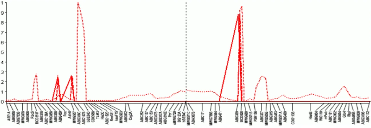
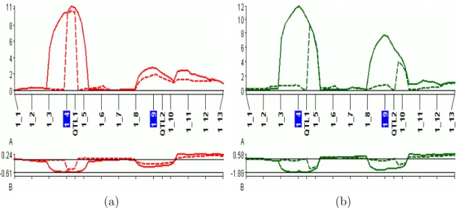
3.4 Multiple-trait PMLE, shrinkIM, and MIM on Steptoe ×Morex dataset . . . 45

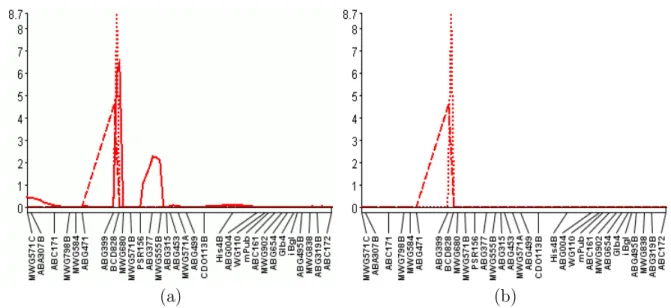
3.5 Single-trait PMLE and shrinkIM on chromosomes 2 and 3 of Steptoe×Morex dataset . . . 46

3.6 Single-trait MIM on chromosomes 2 and 3 of Steptoe ×Morex dataset . . . 46

3.7 Pleiotropy and Q×E tests with PMLE and shrinkIM on Steptoe × Morex dataset . . . 47

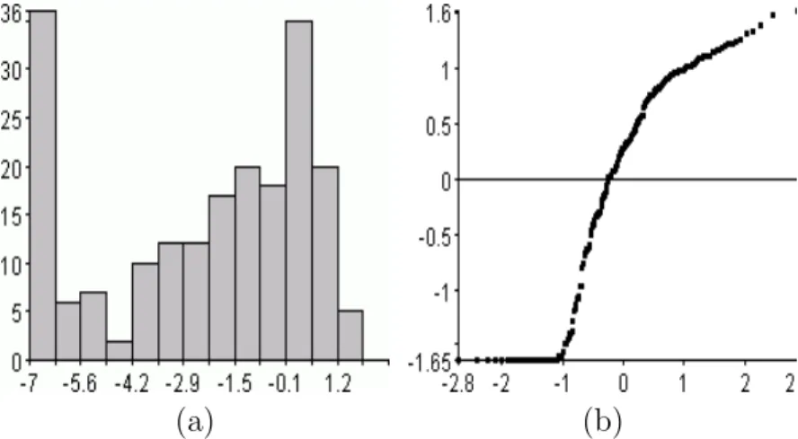
4.1 Histogram and QQ plot of skewed trait distribution . . . 61

4.2 Histogram and QQ plot of log-transformed skewed trait distribution . . . 61

4.3 Comparison of CIM and MIM on log-transformed and original skewed trait data . . . 62

4.4 Comparison of GLZ-based CIM and MIM on skewed trait data . . . 62

4.5 Comparison of multicategorical data analysis between methods with and without normality assumption . . . 64

5.1 Conversion of a QTL LOD plot into a heat map for one e-trait. . . 68

5.2 EQTL heat map in QGene . . . 68

5.3 A global gene regulatory network produced by GGM after removal of edges between e-traits lacking common eQTLs . . . 82

5.4 The distribution of cluster cutoff values for data of Gasch and Eisen(2002) 88 5.5 Diagram showing the similarity of putative mating-associated clusters from JFuzzy-K and _Yvert et al.(2003) . . . 89

5.6 The distribution of cluster cutoff values for the data of Brem et al. (2002) . 90 5.7 Yeast metabolic pathways shown in the BioCyc Omics Viewer with high-lighted edges indicating e-traits varying in the data of _Brem et al. (2002) . . 93

5.8 Putative amino-acid- and protein-biosynthesis network constructed by GGM-eQTL . . . 94

5.9 Putative amino-acid-biosynthesis and -metabolism network constructed by

GGM-eQTL . . . 95

5.10 Putative amino-acid-biosynthesis and -transport network constructed by GGM-eQTL . . . 96

5.11 Sulfate-degradation pathway retrieved from BioCyc database . . . 97

5.12 Pathways for arginine and serine biosynthesis from 3-phosphoglycerate, re-trieved from BioCyc database . . . 97

5.13 Putative sterol-metabolism and electron-transport network constructed by GGM-eQTL from data of Brem et al.(2002) . . . 98

5.14 Ergosterol-biosynthesis pathway retrieved from BioCyc database . . . 99

5.15 Putative network for mating process constructed by GGM-eQTL from data of Brem et al. (2002) . . . 99

6.1 QTL analysis in QGene . . . 106

6.2 Trait analysis in QGene . . . 107

List of Tables

1.1 Conversion table for common mating designs . . . 6

3.1 Comparative QTL-detection accuracy of MIM, PMLE, and shrinkIM, from simulation . . . 43

3.2 QTL effect values from comparative simulation study of PMLE and MT-shrinkIM . . . 48

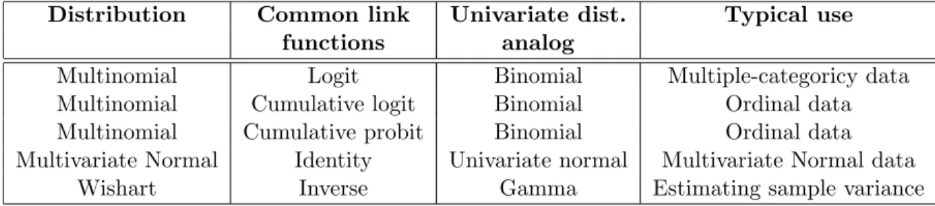
4.1 Typical error term distributions in the generalized linear model, with associ-ated link functions and variances. . . 53

4.2 Multivariate error term distributions and link functions used in generalized linear models. . . 58

5.1 Datasets used for Fuzzy-K bootstrap . . . 86

A.1 Genes in a putative sterol-metabolism and electron-transport cluster . . . 126

A.2 Genes in a putative amino-acid and protein biosynthesis cluster . . . 131

A.3 Genes in putative amino-acid biosynthesis and -metabolism cluster 6 . . . . 137

A.4 Genes in putative amino-acid biosynthesis and -metabolism cluster 9 . . . . 155

A.5 Genes in putative mating cluster 1 . . . 163

A.6 Genes in putative mating cluster 7 . . . 165

List of Program Listings

6.1 Creating a new plug-in category . . . 109 6.2 Creating a new QTL mapping plug-in . . . 109 6.3 A QGene script running single-trait MIM . . . 112

Acknowledgements

I would like to thank my major professor, Dr. James C. Nelson, for his guidance and correction in my thesis. He has given much influence in my graduate education.

I would like to thank my committee members, Drs. Jianming Yu, Doina Caragea, Peter Bradbury, and Lawrence Davis, for their input in this dissertation.

I would like to thank Drs. Barbara Valent and John Boyer for their approval to pursue a second degree in statistics.

Dedication

I dedicate this dissertation to my wife, Elkarisma, who has made countless sacrifices to make this dissertation possible.

Chapter 1

Introduction to quantitative trait

locus analysis

Abstract

In this chapter, the concept of quantitative trait locus (QTL) mapping and its related concepts are introduced. Basic terminology in QTL mapping is described and explained.

1.1

Background

QTL analysis aims to locate and estimate the effects of genes that are responsible for quan-titative traits, such as grain protein content and yield, by means of statistical methods that evaluate the association of genetic variation with trait (phenotypic) variation. Quantitative traits are typically polygenic, i.e., controlled by multiple genes, with varying degrees of influence on the phenotype.

In order to understand QTL analysis, it is necessary to know how genetic variation arises. This is explained in the following sections.

1.2

Chromosome, locus, allele, genotype

A chromosome can be thought of as an array of ordered loci (singular locus). Each locus can be thought of as a variable that can take any of several discrete values called alleles.

For species we consider here, chromosomes come in pairs for which the same loci lie in the same order. For example, humans have 23 pairs, yeast 16, and barley 7.

The two alleles at a locus on a chromosome pair are called the locus genotype. If a genotype has identical alleles, it is homozygous. Otherwise, it is heterozygous.

For example, consider a chromosome pair with only one locus, A. Suppose for this locus there are only two alleles,A anda, in a population of chromosome pairs. In this case, there are three possible genotypes: AA, Aa, and aa. AA and aa are homozygous, while Aa is a heterozygous genotype. Genotype aA is indistinguishable from genotype Aa.

1.3

Gametogenesis and meiosis

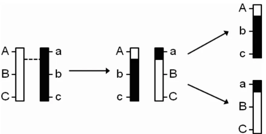
Genotypic variation is created from a process called crossing over. In crossing over, the paired chromosomes exchange segments, as shown in Figure 1.1, and produce two child chromosomes, or gametes. The result of this process is called recombination. The event in which crossing over occurs is called meiosis. Although meiosis takes place in all plant and animal sex organs, recombination can be detected only when the chromosome segments exchanged carry different alleles.

Gametogenesis occurs in both father and mother. One gamete from the father will pair with one from the mother to form the progeny chromosome pair.

Figure 1.1: A pair of chromosomes exchange segments via crossing over. The broken line

1.4

Recombination fraction

There is a certain probability of crossing over between every two loci. Consider a pair of chromosomes with two loci, A and B. This pair forms a new gamete as shown in Figure 1.2. The parental chromosomes have genotypes AaBb. The genotype of the gamete is one ofAB, ab, Ab, or aB. AB and ab are called parental types because the loci are the same as those of the parents, while Ab and aB are recombinant types. Recombinant types are the result of crossing over.

Although the true probability of crossing over is not known, it can be estimated from the proportion of recombinant types observed in a mating experiment. This proportion is called the recombination fraction, or r. Let fXY be the frequency of gamete XY. The recombination fraction between locus A and B, or rAB in this example is then rAB = (fAb+faB)/(fAB +fab+fAb+faB).

Figure 1.2: The assortment of gametes produced in gametogenesis. The upper half shows

the parental chromosome pair, with genotype AaBb; the lower half shows the array of gametes that it can produce. AB and ab represent parental and Ab and aB recombinant gametes.

f(XY) denotes the frequency of gamete XY.

The smaller the recombination fraction, the lower is the probability of a crossover. When

r is very small, the two loci are said to be tightly linked. When the two loci are unlinked, the genotypes of these loci are independently sampled during gametogenesis. In this case,

asymptotically, the frequency of parental types and of recombinant types are the same, or

r = 0.5.

For visualization of markers in a genetic map, it is convenient to cast recombination fractions as genetic distances. Since these fractions do not have an additive relationship, i.e., for loci A, B, and C, rAB+rBC 6=rAC, amapping function is required to convert them into distances to preserve additivity. With one of these functions, recombination fractions between pairs of loci can be used to construct a genetic map. In genetic maps, genetic distances are expressed in terms of Morgans (M) or centiMorgans (cM), after geneticist Thomas Hunt Morgan.

1.5

Mapping population and mating design

A mapping population for QTL analysis starts with a cross of two parents that have con-trasting values for traits of interest. These parents ideally have homozygous genotypes at all loci. In plants such parents are created by repeated self-pollination, orselfing, over multiple generations. These parents are known as inbred lines, or simply lines.

(a) (b)

Figure 1.3: (a) F2 mating design; (b) Converting genotype data to numerical values

A mating design is a description of the crosses used to produce recombinant progeny starting with the inbred parents. Its goal is to create genotypic variation (arising from random parental chromosome sampling) at each locus, and recombination (arising from

crossing over) between loci. The first governs the accuracy of QTL effect estimates and the second that of QTL location estimates.

First, the inbred parents are crossed to form an F1 progeny. When both parents are all

homozygous with differing alleles at every locus, the F1 progeny are all heterozygous. Then,

crosses may be carried out either to self each F1 plant to form F2 progeny (Figure 1.3(a)),

or to cross the F1 with one of the parents to form backcross (BC1) progeny. In the F2, there

are two recombinationally informative meioses per progeny, one for each parent, while in the BC1 there is only one, in the F1 parent.

Recombinant inbred lines (RILs) are another commonly used mating design for QTL analysis, in which repeated selfings are performed over several (usually 6–8) generations from the F1. The repeated selfings yield progeny with homozygous genotypes at almost every

locus. There are two recombinationally informative meioses per progeny per generation, one in each parent per progeny per generation.

Haploid doubling (DH) is also a common mating design. DH creates an instant homozy-gote through methods such as anther culture, in which the male gametes of an F1 progeny

are cultured and then treated with a chemical to induce doubling. In DH, there is only one meiosis per progeny, i.e., from the F1 parent. A DH progeny, like a RIL, can be selfed to

create genetically identical offspring for replicated experiments.

Each mating design produces different proportions of genotypes for each locus. These proportions are the unconditional genotypic probability of each locus. For example, in an F2 population, the expected frequency distribution ofaa, Aa, andAAgenotypes is 1:2:1. In

other words, the genotypic probability distribution for all loci is 0.25, 0.5, and 0.25, for aa, Aa, andAA, respectively. In the BC1, the ratio is 1:1:0, and in the RIL and DH, it is 1:0:1.

1.6

Genotypic assay and numerical conversion

After the mapping population is formed, the genotypes of the progeny at preselected loci are assayed. The loci upon which genotypes are assayed are called DNA markers.

After the genotypes from all progeny are assayed, they are converted to numeric form according to Table 1.1 and Figure 1.3(b). The conversion is done by multiplication of the genotype data by a suitable contrast. For example, for an F2 population, the contrast in

column A is used to measure an additive effect, which is half the difference between the phenotypic means (for some trait) of the two homozygous genotypes AA and aa. The contrast in column D is used to measure adominance effect, which is the difference between the phenotypic means of the Aa genotype and the average of the homozygotes. When only two genotypes are present, such as only Aa and aa in a BC1 design, only the additive effect

can be estimated. These values are used in QTL mapping as the values of the explanatory variables.

1.7

Summary of a QTL mapping process

In summary, QTL mapping is done as follows:

• Select two inbred lines that have contrasting values for traits of interest.

• Make a mapping population from these lines with a suitable mating design.

• If a genetic map is available, select a set of loci as markers that are dense enough to cover the entire map. If a genetic map is not available, there are methods to create and select markers from which a genetic map can be constructed.

Table 1.1: Table for converting genotypes into numerical values for common mating

de-signs. The numbers in column A describe a contrast; i.e., they sum to 0. The numbers in column D describe a contrast corrected for the combination of genotypes Aa and aA in one class.

Mating Design Column A Column D

AA Aa aa AA Aa aa

F2 1 0 -1 -0.5 0.5 -0.5

BC1 0 0.5 -0.5 N/A

• Assay the genotypes of each progeny at the selected markers.

• Assay the phenotypes or traits of interest.

Chapter 2

Review of QTL mapping methods

Abstract

In this chapter, most well-known QTL mapping methods, such as single-marker regression, simple, composite, multiple, multiple-trait composite, and Bayesian interval mapping, are compared and described in depth. The concept of inferring QTL genotypes is also explained.

2.1

Method overview

The statistical model used for QTL analysis is usually a general linear model (GLM), y=

Xβ +, where y represents quantitative trait data (e.g., plant height), X represents the genotypic data as described previously,β represents QTL effects, andrepresents residuals. These are usually assumed to be independent, with ∼ N(0, σ2In), where In is the n×n identity matrix, with n the number of observations. Here, y is an n×1 vector, X is an

n×(cg+ 1) matrix, andβis a (cg+ 1)×1 vector, wherecis the number of effects per marker and g is the number of markers in the model. In the F2 design, c = 2 (e.g., additive and

dominance effects), while in BC1 and RIL, c = 1. The number g of markers in the model

varies according to the QTL-mapping method. In addition to the genotypic values, the X

matrix may contain non-genetic factors whose fixed effects are of interest. The structure of

X varies with the method.

genotypic data of one marker at a time (g = 1). At each marker, a statistic, typically a LOD score, is computed. The LOD score is a log to base 10 of a likelihood ratio test (LRT). In this test, the null hypothesis is that the marker has neither additive nor dominance effect, while the alternative hypothesis is the negation of the null hypothesis. This process is repeated for all m markers; that is, the model is fitted to each marker, resulting in m

tests. If an association between an existing marker and the trait is detected, i.e., if the marker has a LOD score exceeding some predefined threshold, it is inferred that a QTL is located near that marker based on the observation that the genotypes of loci that are closer together are more likely to be inherited together. So for sufficient odds of detection of a QTL, and precisions of location estimates, the sampled markers must be adequately densely distributed.

Multiple-testing issues and correlations among the test statistics due to linkage make it difficult to determine a statistical-significance threshold for QTLs. The conventional threshold of LOD 3 based on the asymptotic distribution may not reflect the true significance threshold (Mangin et al.1994).

The multiple-testing problem can be addressed by false-discovery-rate (FDR) methods

(Benjamini and Hochberg1995;Storey and Tibshirani2003) and permutation

anal-yses (Churchill and Doerge 1994). In FDR methods, the rate of false discovery

(pro-portion of false positives) is estimated for determining the correct cutoff (Benjamini and Yekutieli2005). In permutation analysis, the LOD score threshold is empirically sampled

under the null hypothesis. In general, permutation analysis is the preferred method because of the correlation among the statistics due to linkage.

Inferring the QTL genotype within a marker interval may improve QTL detection ac-curacy, especially when obtaining a dense map of a particular species is not possible for technical and/or economic reasons. It requires a controlled mating so that the prior proba-bility of each genotype for each marker is known. This probaproba-bility enables the inference of QTL genotypic probability at any given point within marker intervals. Such inference is

use-ful in QTL interval mapping (IM). In QTL IM, each chromosome is divided into equal-sized intervals, measured in units of genetic distance.

Inference of QTL genotype (_Lander and _Botstein1989) relies on the posterior prob-ability distribution of QTL genotype given the genotypes of markers flanking the QTL, the recombination fraction between the QTL and the flanking markers, and the unconditional genotypic probability associated with the mating design. This approach is also useful for computing the genotypic probability distribution of missing marker data.

Consider a QTL Q between markers A and B, with two alleles each in the population. LetAand B denote alleles contributed by the first parent and a and b those by the second. Let dXY and rXY denote the distance and the recombination fraction between X and Y. A mapping function (_Haldane1919) is used to convert the distance into the recombination fraction by rXY = (1−exp(−2dXY))/2, where dXY is expressed in Morgans. The expected frequency of any gamete can be expressed in terms of recombination fractions. For example, at meiosis in the F1, the probabilities of the two nonrecombinant gametesAQB andaqb are

both (1−rAQ)(1−rQB)/2 reflecting the absence of recombination between both AQ and QB. Thus, given the flanking marker genotypes AA and BB, the probability that GQ, the genotype at QTL Q, equals QQ is

P(GQ =QQ|A=AA, B=BB) = (1−rAQ)2(1−rQB)2/4

because it is formed from two AQB gametes. Likewise, the probability of Qq and qq geno-types are P(GQ =Qq|A=AA, B=BB) = (1−rAQ)(1−rQB)rAQrQB/2 and P(GQ =qq|A=AA, B=BB) = r2AQr 2 QB/4

The preceding method is practical only for simple mating designs such as BC1 and F2.

A matrix method accomodates more complex mating designs and incompletely informative marker genotypes. A Markov-chain approach (Jiang and Zeng 1997) was developed as

a generalization allowing use of the information from all markers in the chromosome. The computation is as follows. Let pL

k and pRk be the probability of QTL k, given the markers to its left and to its right. Let A#B denote the Hadamard (componentwise) product of two vectors, A and B. Let qk be the unconditional genotypic probability from the mating population. The expected frequency of each genotype of QTL k is a 3×1 vector given by

v= qk#(pLk#pRk) q0 k(p L k#p R k)

. This probability vector is then multiplied by the contrast vectors in Table 1.1, as illustrated in Figure 2.1.

The inference of QTL genotypic probability within marker intervals is required for QTL interval mapping (IM). In effect, IM interpolates the LOD score within marker intervals. The points within the intervals are treated as “virtual markers” with all-missing data. The Markov-chain approach is used to infer the QTL probability distribution, which is a 3×1 vector denoting the respective probabilities of AA, Aa, and aa genotypes.

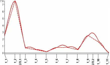
Simple interval mapping (SIM) is the IM analog of SMR. Just as in SMR, a statistic such as LOD is computed at each test position, instead of at each marker. SIM may detect a few more QTLs than SMR, as shown in Figure 2.2.

Composite interval mapping (CIM) (Zeng1994;Jansen1994;Jansen andStam1994)

improves upon SIM by including in the modelbackground markers orcofactors,i.e., markers in the genetic map that are selected to reduce residual genetic variation arising from QTLs not linked to the QTL being tested. Such reduction allows more precise QTL location estimation by giving narrower peaks. Multiple interval mapping (MIM)(Kao et al. 1999)

improves upon CIM by fitting multiple putative QTLs simultaneously via an EM algorithm. Bayesian interval mapping (BIM) (Satagopan et al. 1996) uses a Markov-chain Monte

Carlo (MCMC) approach to sample the posterior probabilities of the QTL genotypes, effects, and locations. These are accepted with a proposal probability computed with a Metropolis-Hastings (MH) method. An improvement of BIM using reversible-jump MCMC (RJMCMC) was proposed (Sillanp¨a¨a and Arjas 1998; Stephens and Fisch 1998) to address the

Figure 2.1: An illustration of a Markov-chain method of (Jiang and Zeng 1997) for

inferring QTL genotype. In this example, QTL Q1 and Q2 are flanked by markers A and

B. The genotypic probability distribution (GPD) vectors of Q1 and Q2 are computed with a

Markov-chain method. Intuitively, since Q1 is closer to marker A, its GPD should resemble

marker A’s. Similarly, since Q2 is closer to marker B, its GPD should resemble marker B’s.

The value for the corresponding A column for the QTL is its GPD multiplied by (−1,0,1)0. Likewise, the value for the corresponding D column for the QTL is its GPD multiplied by (−0.5,0.5,−0.5)0. In all interval-mapping methods, these values replace the values from the substitution rule described in the text. Notice that for individual 2, the values in A and D columns for Q1 and Q2 are different because of differing flanking marker genotypes.

2.2

Least-squares-based SMR, SIM, and CIM

In single-marker regression (SMR), the number of markers in the model, g, is one and the model reduces to y=µ1+axa+dxd+. The 1vector signifies a column of ones and µis an overall mean effect. Then×1 vectorsxaandxd are genotypic values converted as shown in Table1.1 and Figure 1.3 (b). The scalarsaand d are the additive and dominance effects of interest to geneticists. If the mating design does not have column D in Table1.1, such as in BC1 and RIL, the term dxd is omitted, since the dominance effect cannot be estimated for that design. The statistics are computed at each marker in turn across the genetic map. An example of an SMR plot appears in Figure 2.2.

Simple interval mapping (SIM) uses the same model used in SMR except that the values in vectors xa and xd are computed from QTL genotype probability estimates described previously.

In composite interval mapping (CIM), the linear model is y=µ1+axa+dxd+X∗β∗+. The vectorsxa andxd are as in SIM.X∗ is ann×cmmatrix of background markers, where

cis the number of QTL effects (i.e., the number of columns in Table1.1for the given mating

Figure 2.2: Typical QTL-mapping profile. In this example, both single-marker regression

(SMR) and simple interval mapping (SIM) detect a QTL 1, but only SIM can detect QTL 2. The plot is created from the LOD profiles of a simulated 200-progeny F2 population. Broken

design) and m is the number of background markers. These can be selected manually or with model-selection methods, such as stepwise- or forward-selection. The entries of the X∗

matrix are obtained by the same conversion rule used for converting marker genotypes to numbers in SMR. Thus, in the absence of background marker matrix X∗, CIM reduces to SIM.

SMR, SIM, and CIM models are regression models and can be solved by least-squares methods. Let X= [1|xa|xd|X∗] andβ0 = [µ|a|d|β∗

0

]. Thus, these models can be written as

y=Xβ+. The solution of the QTL effects is expressed byβ = (X0X)−1_X0_y.

Na¨ıve implementation of a least-squares method is slow and is numerically unstable owing to the finite precision of real numbers in computers. An ordinary least-squares solution involves three matrix multiplications and one matrix inversion. Precision loss occurs at every numerical operation, especially in matrix inversions. Moreover, matrix multiplications and inversions are among the most computationally expensive basic matrix operations.

To improve numerical accuracy and computation speed, QR decomposition is usually used by common statistical software. X is decomposed into Q and R, where Q is an orthogonal matrix (i.e., Q0Q=I) and R is an upper triangular square matrix. Thus:

β= (X0X)−1X0y= (R0Q0QR)−1R0Q0y

= (R0R)−1R0Q0y=R−1R0−1R0Q0y=R−1Q0y Rβ=Q0y

The solution forβ can be obtained by backward substitution. Numerical accuracy is im-proved because matrix inversion is no longer necessary and only two multiplications are needed. Computation speed is improved because partial QR decomposition can be per-formed for each marker or interval. Result computation from partial decomposition is much faster than from full decomposition.

The null hypothesis is that the QTL effects are zero (a=d= 0),i.e., there is no QTL. In SMR and SIM, the null model is y=µ1+. In CIM, the null model isy=µ1+X∗β∗+. The corresponding F statistics are computed. The LOD score can be obtained as LOD =

n 2 log 10log F dfR dfE + 1

(Doerge 1995), wheren is the number of progeny, dfR and dfE are the degrees of freedom for regression and error, and F is the F statistic.

2.3

EM-based SMR, SIM, and CIM

Single-marker regression (SMR), simple (SIM), and composite interval mapping (CIM) can also be solved by an EM algorithm, as derived in Kao and Zeng (1997). Assuming the

CIM model and iid Normal for the error term, the joint likelihood function (Kaoand Zeng

1997) for θ= (p, a, d,β, σ2_{) of n individuals is as follows:} L(θ|y,X) = n Y j=1 " ₃ X i=1 pjiφ yj−µji σ #

where φ(·) is a standard normal pdf, µj1 = a − d/2 + Xj∗β ∗ , µj2 = d/2 + Xj∗β ∗ , and µj3 = −a−d/2 +Xj∗β ∗

. The index i iterates over genotypes AA, Aa, and aa. Thus, µji and pji denote the mean and the prior probability (given flanking markers) of the ith QTL genotype.

An EM algorithm can then be used to obtain maximum-likelihood estimates (MLE) of

θ. The normal mixture of the preceding equation can be treated as an incomplete-data problem (_Dempster et al. 1977) since the QTL genotypes are unknown. Let

gj(x∗_j, z_j∗) =    pj1 if x∗j = 1 andz ∗ j =− 1 2 pj2 if x∗j = 0 andz ∗ j = 1 2 pj3 if x∗j =−1 and z ∗ j =− 1 2

be the distribution of QTL genotype specified byx∗_j andz_j∗. The unobserved QTL genotypes, (x∗_j andz∗_j), are treated as missing data (Kao and Zeng1997), denoted byq∗j, and traityj, selected background markers, and explanatory variables Xj are treated as observed data, denoted by y(obs,j). The conditional distribution of observed data given missing data is

yj|(θ, Xj, x∗j, z ∗ j)∼N(x ∗ ja+z ∗ jd+Xjβ, σ2) Thus, the density of the complete data, y(com,j), is

f(y(com,j)|θ) = f(y(obs,j)|θ, Xj, x∗j, z ∗ j)g(x ∗ j, z ∗ j)

The E step of the EM algorithm is as follows.

Qθ|θ(t)=

Z

logL(θ|ycom)f(q∗|yobs,θ =θ(t))dq∗

= Z log " _n Y j=1 φ yj−µj σ gj(x∗j, z ∗ j) # ×f(q∗|yobs,θ =θ(t))dq∗

By Fubini’s theorem governing changes to the order of integration,

Q θ|θ(t) = n X j=1 Z log φ yj−µj σ gj(x∗j, z ∗ j) ×f(q_j∗|y(obs,j),θ =θ(t))dqj∗ = n X j=1 3 X i=1 log φ yj−µj σ pji × pjiφ yj−µ(t)_ji σ(t) 3 X k=1 pjkφ yj −µ (t) jk σ(t) ! = n X j=1 3 X i=1 log φ yj−µj σ pji ×π_ji(t)

Observe that by Bayes’ rule,πji is the posterior probability of the QTL genotype. Assuming that the true QTL genotype is the ith genotype, write

fq∗_j|y(obs,j),θ =θ(t) = fy(obs,j)|q∗j,θ =θ (t)_fq∗ j|θ=θ (t) f y(obs,j)|θ=θ(t) = φ yj−µ(t)_ji σ(t) pji 3 X k=1 pjkφ yj−µ (t) jk σ(t) ! =πji

In the M step, the MLE solution is obtained by differentiation of Q

θ|θ(t)

to θ, yielding a(t+1) = n X j=1 π_j(t₁)−π_j(t₃) yj−Xjβ(t) −1 2 π_j(t₃)−π_j(₁t)d(t) n X j=1 π_j(t₁)+π(_jt₃) = y−Xβ(t) 0 Π(t)d1−10Π(t)(d1#d2)d(t) 10_Π(t)_(d 1#d1) d(t+1) = n X j=1 1 2 h −π_j(t₁)+π_j(t₂)−π(_jt₃) yj −Xjβ(t) −π_j(t₃)−π_j(t₁)a(t)i n X j=1 π_j(t₁)+π(_j2t)+π_j(t₃) = y−Xβ(t) 0 Π(t)_d 2−10Π(t)(d1#d2)a(t) 10_Π(t)_(d 2#d2)

where # denotes the Hadamard (componentwise) product of two vectors, Π = {πji}n×3,

d1 = (1,0,−1)0, and d2 = (−1₂,1₂,−1₂)0.

Let e(t)_{= (a}(t)_{, d}(t)₎0_{. The equations above simplify to}

e(t+1)=r(t)−M(t)e(t) where r(t) =   (y−Xβ(t)₎0_Π(t)_d1 10_Π(t)_(d1#d1) (y−Xβ(t)₎0_Π(t)_d2 10_Π(t)_(d2#d2)   and M(t) = " 0 1₁00Π_Π(t)(t)(₍d1_d1##_d1d2)₎ 10Π(t)(d2#d1) 10_Π(t)_(d2#d2) 0 # β(t+1) = (X0X)−1X0y−Π(t)De(t+1) σ2(t+1) = 1 n y−Xβ(t+1) 0 y−Xβ(t+1)−y−Xβ(t+1) 0 Π(t)De(t+1) +e0(t+1)V(t)e(t+1) where D= (d1,d2) and V(t) = 10Π(t)(d1#d1) 10Π(t)(d1#d2) 10Π(t)(d2#d1) 10Π(t)(d2#d2)

Note that V, but not M, is symmetric.

In the first iteration, Π is filled with the genotypic distribution obtained from the Markov-chain approach described previously. The vectors β and e are filled with the esti-mates from the least-squares method.

The estimates of the parameters and the Π matrix are updated as described until con-vergence. The null hypothesis is a=d= 0 and the log likelihood for the null hypothesis is also computed. A likelihood ratio score (LR) is computed and the LOD score is obtained by LOD = LR/(2 log 10).

2.4

MIM

Multiple interval mapping (MIM) (Kao et al. 1999) builds upon the EM solution of

com-posite interval mapping (CIM). Instead of fitting background markers, it fitsq QTLs simul-taneously. Thus, the indexiin the EM solution above runs from 1 to 3q _{(or 2}q_{in the absence} of a dominance effect), accounting for all possible QTL genotype combinations. The joint likelihood function now becomes:

L(θ|y,X) = n Y j=1 " ₃q X i=1 pjiφ yj−µji σ #

The updating rule for the posterior probability of QTL genotype becomes:

π_ji(t+1) = φ yj−µ(t)_ji σ(t) pji 3q X k=1 pjkφ yj −µ (t) jk σ(t) ! ∀i∈ {1, . . . ,3 q_}

The genetic design matrixD3q_×2 =1_q⊗ {d₁,d₂}, if both additive and dominance effects are present, or D3q_×1 =1_q⊗ {d₁}, if only an additive effect is present. The symbol ⊗ denotes the Kronecker product.

Consequently:

r =      y−Xβ(t) 0 Π(t)_d 1 10_Π(D i#Di)      e×1 M= 10Π(t)_(d i#dj) 10_Π(t)_(d i#di) e×e

where e is the number of columns of D.

The formulas above are a straightforward extension to allow estimation of both dom-inance effect and non-genetic factors. The original paper describes only the formulas for designs with only additive effect present and no non-genetic factors. Here, matrix X con-tains only non-genetic factors, while the other matrices and vectors are kept the same as those of CIM. If there are no non-genetic factors, then X=1.

Since fitting too many QTL at once is computationally expensive, MIM uses a stepwise or “chunkwise” selection method to add QTLs into the model. In stepwise selection, QTL is added to the model one by one. In chunkwise selection, several QTLs are added to the model at a time. The QTL selection proceeds as in usual model-selection procedures.

2.5

MT-CIM

Multiple-trait QTL analysis is QTL analysis applied to several traits simultaneously. Such analysis has been shown (Jiang and Zeng 1995) to improve the statistical power of QTL

detection test and the precision of parameter estimation by taking into account the corre-lation structure among the traits. In addition, such analysis provides formal procedures to test for pleiotropy (i.e., whether a QTL affects all selected traits) and QTL-by-environment (Q×E) interaction.

Multiple-trait CIM (MT-CIM) (Jiang and Zeng1995) builds upon the EM solution of

single-trait CIM. The model is the same as that of CIM, except that all matrices and vectors are expanded to t variates. If t denotes the number of traits (i.e., variates), the model is expressed by

Y

n×t= n×x11a×t+n×z11d×t+n×(2Xk+p+1)(2k+Bp+1)×t + E

n×t

the number of non-genetic covariates. Notice that if t = 1, this model reduces to the CIM model.

Although the encoding of QTL genotypes is different, the steps to derive the solution are essentially the same. In the original paper, xj takes values of 2, 1, and zero for respective QTL genotypes AA, Aa, and aa. zj takes value 1 if the QTL genotype is Aa, otherwise 0.

The joint likelihood function of the data is

L1 =

n

Y

j=1

[p2jφ2(yj) +pijφ1(yj) +p0jφ0(yj)]

where the pij are the prior probability of QTL genotypes of AA, Aa, and aa and φi(·) is multivariate normal with variance σ and mean uj2 = XjB+ 2a, uj1 =XjB+a+d, and

uj0 =XjB, respectively.

The log-likelihood function is given by

ln(L1) = k∗− n 2 ln ˆ V + n X j=1 ln p2jexp 1 2[yj−2ˆa−XjBˆ]Vˆ −1_[y j −2ˆa−XjBˆ]0 +p1jexp 1 2[yj −ˆa− ˆ d−XjBˆ]Vˆ−1[yj−ˆa−dˆ−XjBˆ]0 +p0jexp 1 2[yj −XjBˆ]Vˆ −1_[y j−XjBˆ]0 =k∗−n 2 ln ˆ V − 1 2 n X j=1 [yj −XjBˆ]Vˆ−1[yj−XjBˆ]0 + n X j=1 ln p2jexp[2ˆa ˆV−1[yj −ˆa−XjBˆ]0] +p1jexp[(ˆa+dˆ)Vˆ−1[yj − 1 2ˆa− 1 2 ˆ d−XjBˆ]0] +p0j

Differentiating the log-likelihood function with respect to its parameters yields a(t+1) = q 0_(t+1) 2 2q0₂(t+1)1(Y−XB (t)₎ d(t+1) = " q0₁(t+1) q0₁(t+1)1 − q0₂(t+1) 2q0₂(t+1)1 # (Y−XB(t)) B(t+1) = (X0X)−1X0[Y−(2q(₂t+1)+q(₁t+1))a(t+1)−q(₁t+1)d(t+1)] V(t+1) = 1 n h (Y−XB(t+1))0(Y−XB(t+1))−4(q0₂(t+1)1)a0(t+1)a(t+1) −(q0₁(t+1)1)(a(t+1)+d(t+1))0(a(t+1)+d(t+1)) i

whereq(₂t+1) andq(₁t+1) are the respectiven×1 vectors ofq₂(t_j+1)andq₁(_jt+1), and fori= 0,1,2, qij = pijφ(it)(yj) 2 X k=0 pkjφ(_kt)(yj)

There are several modes of hypothesis testing in multiple-trait analysis:

1. Joint QTL mapping Is there any QTL detected for any trait?

Under joint-mapping the hypotheses to be tested are H0 : a = d = 0 vs. HA : otherwise. In this case, the log-likelihood under H0 is given by

ln(L0) = ln " _n Y j=1 φ0(yj) # =k− n 2 ln| ˆ V0| −nm/2

where Vˆ0 = (Y−XB0)0(Y−XB0)/n and B0 = (X0X)−1X0Y. The LOD score is

obtained from LOD =− 1 ln(10)ln L0 L1 .

2. Test of pleiotropic effects Is there any QTL that affects all traits?

The hypotheses to be tested are H0 :ai = 0 or di = 0 for some trait i vs. HA :a6= 0 and d6= 0 (i.e., testing if the QTL effects are zero in at least one trait). In this case, there are multiple null hypotheses. The log-likelihood ratio score can be obtained from the formulas derived above, with the appropriate effects set to zero. Although the original paper (Jiang and Zeng 1995) did not explicitly mention a combined

LOD score, it is usually taken as the minimum of the LOD scores at a particular marker or interval.

3. Test of close linkage versus pleiotropy Is the detected pleiotropic QTL not an

artefact of several closely-linked QTLs?

A QTL that affects all traits is not necessarily a pleiotropic QTL. It may be an artefact of several closely linked QTLs. This test is designed to distinguish the two, especially if the pleiotropic LOD score peak is wide.

Let pos(i) be the position of the currently tested QTL for trait i. The hypotheses to be tested are H0 : pos(i) = pos(j), ∀i, j ∈ {1, . . . , t} vs. HA : otherwise. In this case, the position of QTL for traiti is shifted a little bit (1–2 cM) to either side and tested with the QTL for trait j. A LOD score is then computed in a similar manner. If H0

is rejected, then the QTL involved is not a pleiotropic QTL.

4. QTL by environment (Q×E) analysis Does the QTL affect one trait differently

from the others?

This test is particularly useful when the traits being tested are the same trait (e.g., grain yield) in the same set of individuals (e.g., replicated lines) but measured in different environments.

Let ai and di be the additive and dominance effect of a given QTL for a given trait. The hypothesis to be tested is

H0 : (ai =aj =a) and (di =dj =d), ∀i, j ∈ {1, . . . , t} vs. HA: not H0.

replaced by a and d. In the CM step a(t+1) = q 0_(t+1) 2 2c(t)_q0(t+1) 2 1 (Y−XB(t))(V(t))−11 d(t+1) = " q0₁(t+1) c(t)_q0(t+1) 1 1 − q 0_(t+1) 2 2c(t)_q0(t+1) 2 1 # (Y−XB(t))(V(t))−11 where c(t)₌₁0_V(t)_1.

So, under H0, the log-likelihood now becomes:

ln(L0) =k∗− n 2ln| ˆ V| − 1 2 n X j=1 (yj−xjBˆ)Vˆ−1(yj−xjBˆ)0 + n X j=1 lnhp2jexp[(2a)10Vˆ−1(yj−10a−xjBˆ)0] +p1jexp[(a+d)10Vˆ−1(yj−10(a+d)/2−xjBˆ)] +p0j i

The LOD score is obtained as LOD =− 1 ln(10)ln L0 L1 .

2.6

BIM

In Bayesian interval mapping (BIM), Bayes’ rule, instead of least squares or EM algorithm, is used to derive the solution, although the model used is the same as in CIM. Bayesian solutions require the posterior density of each parameter, obtained from the application of Bayes’ rule. Samples are then generated from this density to yield parameter estimates. If the density resolves to a known one, the samples can be easily generated. However, it often does not. In this case, a sampling method based on Markov chain Monte Carlo (MCMC) approach is used to draw samples from approximate distributions of the parameters and use the samples to correct subsequent draws to better approximate the target posterior distribution. In MCMC, the samples are drawn sequentially, with the distribution of the sampled draws depending on the preceding values (states) drawn; hence, the draws form a Markov chain. Under the detailed-balance property, i.e.,where any given state of the chain

can be revisited infinite times from any state in a finite number of steps, the approximate distributions are improved at each step and converge to the target distribution (_Gelman et al. 2003, pp. 285–286).

Gibbs sampling is an MCMC-based method in which samples of a parameter θj are drawn from the conditional distribution of θj given the values of all other parameters, θ−j, given data, y, p(θj|θ−j,y). This means that Gibbs sampling requires p(θj|θ−j,y) for each parameterj in the model. For many problems involving standard statistics, this conditional distribution resolves to a known form that is easily sampled.

For cases where conditional distributions are unknown, the Metropolis–Hastings (MH) algorithm is used. In MH, a vector of proposal valuesθ∗ is sampled at iterationtforθ from a proposal distribution of Jt(θ∗|θt−1). The proposal θ∗ is accepted (i.e., θt = θ∗) at rate min(1, r), where:

r= p(θ ∗_|

y)/Jt(θ∗|θt−1)

p(θt−1|y)/Jt(θt−1|θ∗)

and θt−1 is the values of the parameter vector at the previous iteration. In essence, the MH algorithm is an adaptation of a random walk that uses an acceptance–rejection rule to converge to the specified target distribution. It has been shown that Gibbs sampling is a special case of the MH algorithm with r= 1 (Gelman et al. 2003, pp. 292–293).

QTL mapping may be approached with a hybrid MH–Gibbs method (_Satagopan et al. 1996). QTL locations and genotypes are sampled with Gibbs samplers, while QTL effects are sampled with the MH algorithm.

The MCMC method approach discussed so far assumes that the dimension of parameter spaceθ is known. In QTL analysis, this implies that the number of QTLs is already known, which is rarely the case. For addressing this variable dimensionality, reversible jump MCMC (RJMCMC), a generalization of the MH algorithm allowing random walk across dimensions, was developed (_Green 1995). It relies on a one-to-one, deterministic, and differentiable function fn→m(·) that transforms the parameter from dimension n tom. Let Jn→m(·|n,θn) be the proposal distribution that proposes parameter values in dimensionmgiven the values

of parameters in dimension n, q(m|n) the probability of jumping from dimension n to m,

p(n,θn|y) the posterior probability of parameter θn in dimension n, Jfn→m the Jacobian term specified by the transformation function fn→m(·). The move from dimension n to m is accepted (i.e., θt =θm) at a rate of min(1, r), where:

r= p(m,θm|y)/[q(m|n)Jn→m(un,m|n,θn)]

p(n,θn|y)/[q(n|m)Jm→n(um,n|m,θm)]

× Jfn→m

and un,m is the proposal values that “complete” the parameter values from dimension n when transformed to dimension m.

To ensure the detailed-balance property, reversibility of the Markov chain must be main-tained. This means that at every iteration, a jump from dimensionm ton must be followed by a reverse jump from dimension n to m. In between, there must be a step to update the parameter values within dimensions.

According to (_{Sillanp¨a¨a} and _Arjas 1998), the steps in each iteration in the QTL analysis are:

1. QTL birth,i.e.,introducing one QTL into the model

2. Moving one QTL position at random

3. Sampling QTL effects

4. QTL death, i.e.,deleting one QTL at random from the model

The first and last steps are implemented as RJMCMC acceptance tests. The others are implemented in MH algorithms.

In each of these steps, the ratio of the posterior probabilities reduces to the ratio of likelihoods of the two states. For both QTL birth and death, the Jacobian term of the RJMCMC is 1 since the locations of existing QTLs do not determine the location of a proposed new QTL, nor does the deletion of one QTL influence the positions of the remaining QTLs. The ratios q(n|m)/q(m|n) in QTL birth and death steps are λ/(Nq(t−1) + 1)2 and (Nq(t−1))2/λ, whereN(

t−1)

belief of the number of QTLs. Although (_{Sillanp¨a¨a} and _Arjas 1998) gave a formula to estimate λ, it can be estimated by the number of markers given by a cofactor-marker selection process. The ratio of the proposal distribution can be used to restrict the search space, as in Jm→n(um,n|m,θm)] Jn→m(un,m|n,θn)] = 1, if 0≤Nq(t) ≤Nqmax 0, otherwise

where Nqmax is the maximum number of QTLs allowed in the model. When the position or the effect of a QTL are being updated, the ratio of the proposal distributions is assumed to be 1.

The first b iterations are discarded since the Markov chain has not reached convergence. After the first b iterations, only samples at every t iterations are stored to avoid autocorre-lation in samples between adjacent iterations. If n samples are required, the steps are run

nt+b times. In MCMC term, b represents burn-in, and t thinning iterations.

There is no consensus on how b andtshould be set. Although rules have been proposed, such as by Raftery and Lewis (1995), it is still a contentious subject. Sillanp¨a¨a and Arjas(1998) suggest 500,000 to 1,500,000 iterations with no burn-in or thinning iterations.

The default setting in R/qtlbim (Yi et al. 2005) isb= 600,t = 20, andn = 3000. However,

in most cases such defaults will be unsuitable for the data. The only way to determine the setting is to examine the plot of the number of QTLs, general mean, and the residual variance across iterations.

2.7

Summary

Single-marker regression (SMR), and simple (SIM), composite (CIM) and multiple interval mapping (MIM) can be solved using the same general linear model framework. SMR and SIM use essentially the same model to detect QTL: the former uses marker data, while the latter uses interpolated QTL genotype estimates. CIM and MIM also use the same model. CIM uses marker data, while MIM uses the calculated QTL estimates as the cofactors.

1995). MT-CIM exploits the correlation structure to improve the accuracy of QTL detection. In addition, it provides additional tests that cannot be performed for single traits, such as pleiotropy and QTL-by-environment interaction.

In the absence of multiple traits, MT-CIM reduces to single-trait CIM and its perfor-mance and accuracy are the same as that of CIM. Multiple-trait analyses, such as pleiotropy and QTL-by-environment tests, also can no longer be performed.

Although SIM and CIM are still widely used today, they have less power than, and have been largely superseded by, MIM (_Kao et al. 1999). SIM and CIM may be useful for preliminary analyses because they can be computed rapidly. Although MIM computation is much slower than that of SMR, SIM, or CIM, modern computers can perform MIM computation in seconds to minutes.

Chapter 3

Shrinkage interval mapping

Abstract

The conventional solution to the QTL-mapping model-selection problem, in which only a few QTLs are selected from all QTLs, obtained from stepwise or forward variable-selection methods has been shown to perform poorly due to bias introduced by favoring QTLs that are associated with the largest statististics. A proposed remedy to this problem is penalized regression, in particular the penalized maximum-likelihood method (PMLE). However, this method tends to overpenalize, and thereby may fail to detect, QTLs with smaller effects. As an attempt to overcome this defect, I develop a two-stage hybrid method between MIM and partially penalized regression that can be considered as a generalization of PMLE. A multiple-trait extension is also developed. Simulated experiments showed that it may obtain a more precise QTL-location estimate, but may overestimate the QTL effects. This method has a marginal advantage over PMLE in detecting QTLs with smaller effects. Both PMLE and this method (shrinkIM) are shown to be superior to multiple-interval mapping (MIM).

3.1

Introduction

Consider the linear model Y=Xβ+, where Y is a n×1 trait vector, X an×m marker matrix, β a m×1 vector of regression coefficients, and a n×1 random error vector with

∼N(0,Inσ2). For an oversaturated model, wherem > n, ordinary least-squares estimates of β cannot be calculated as (X0X)−1_X0_{Y because matrix X}0_{X is singular.}

Composite interval mapping (CIM) was proposed to overcome this situation by stepwise or forward variable-selection methods. However, it has been shown (_Hoerl et al. 1986) that such methods perform poorly due to the bias introduced by favoring variables (or in this case QTL) that are associated with the largest statistics.

Another solution, ridge regression (_Hoerl 1962), proposed to overcome this problem is the imposition of penalties on the regression coefficients. Let τ be a penalty parameter. The restricted least-squares estimate is (X0X+τIn)−1X0Y under the quadratic constraint

P

jβ

2

j < τ onβ, for j = 1, . . . , m. Ridge regression has been proposed (Boer et al. 2002) for QTL epistasis analysis, with varying penalties on regression coefficients.

Because the inversion of matrix X0X+τIn required by ridge regression becomes time-consuming as m grows, _Xu (2003) developed a Bayesian shrinkage regression method for simultaneously estimating the genetic effect associated with the markers along the whole genome map. Each marker effect is allowed to have its own variance parameters so that the variance can be estimated from the data. This method was extended (Wang et al. 2005)

to allow localizing a QTL within an interval, using Metropolis–Hastings sampling since the QTL location parameter does not have an explicit posterior distribution.

To eliminate the need of intensive computation imposed by the Bayesian method, the penalized maximum-likelihood estimation (PMLE) method (Zhang and Xu 2005) was

developed. It imposes a prior normal N(µj, σ2j) penalty on each QTL effect j, allowing the penalty to vary across the βj. An EM-based algorithm is used to estimate regression coefficients and other parameters. PMLE is similar in spirit to the multiple-marker Bayesian shrinkage method in that both shrink small marker or QTL effects to zero. PMLE was shown (Zhang and Xu2005) to be comparable to the shrinkage method in terms of performance.

The initial PMLE method could localize a QTL only to a marker and not between markers. An extension was developed (Zhang 2006) to accommodate QTLs within intervals.

While both shrinkage and PMLE methods offer much power for QTL detection, the QTL effects can sometimes be underestimated (_Zhang and _Xu2005). Although this is not serious if the effect is large, it can be highly misleading for small effects.

To overcome the limitation of PMLE, an unpublished method called shrinkage interval mapping (shrinkIM) (_Guo et al. 2007) was proposed. It used PMLE as QTL selector and used unpenalized QTL effect estimates to find other QTLs with smaller effects. This method exploited partially penalized regression to leave QTL effect estimates unpenalized while penalizing spurious effects.

Here, I propose an improvement to shrinkIM that combines PMLE with multiple interval mapping (MIM) (_Kao et al. 1999). This method is a multiple-pass method. In the first pass, PMLE is used to detect QTLs with higher effects. In the second pass, a hybrid between MIM and partially penalized regression is used to fit without penalty the QTLs found in the first pass while simultaneously searching for additional QTLs with smaller effects. This simultaneous unpenalized QTL fitting is analogous to that of MIM and is intended to improve precision and power. Further passes repeat the second until no more QTLs are found.

3.2

Methods of shrinkage interval mapping

Consider m QTL, Q1, . . . , Qm, located at positions p1, . . . , pm of m intervals across the genome that have been not identified by the PMLE method in the previous iteration. As-sume an F2 population of n individuals. There are 3m possible different QTL genotypes

in the population. These QTL genotypes determine a quantitative trait y. Assuming no interaction, the statistical model can be expressed as

yi =µ+xiβ+ m X j=1 (αjzij+δjwij) +i, i= 1. . . n, (3.1) or in matrix form y=Xβ+Zα+Wδ+ (3.2)

where µis the mean,xi andβ are the genotypes and unpenalized effects of the QTL found in previous iterations, zij is coded as 1,0, and −1 for current QTL genotypes QjQj, Qjqj, and qjqj, respectively, wij is coded as 1₂ for heterozygotes and −1₂ otherwise, αj and δj are the additive and dominance effects of QTL j, andi is the environment deviation, assumed to follow N(0, σ2_).

The encoding of zij and wij follows Cockerham’s model (Kao and Zeng 2002), which ensures orthogonality in modeling the genetic parameters. It means that we can treat the

αs and δs as independent variables.

The putative QTL genotypes are not observed because the QTL lie within marker in-tervals. Given observed flanking marker genotypes, the conditional distributions of QTL genotypes can be inferred with a Markov chain method (_Jiang and _Zeng1997), assuming no crossover interference.

The model is a multiple-QTL model and its likelihood is that of a finite normal mixture. Let q be the vector of QTL genotypes, λ the vector of the positions of the QTL,α and δ

the vectors of additive and dominance effects of all m QTLs,β the effects of the confirmed QTLs, andσ2 be the variance. Letκ= (q,λ,α,δ,β, σ2). Assuming that the putative QTL genotypes, given the flanking marker genotypes, are independent, that no penalty is imposed, and that noninformative priors are chosen, the posterior probability of the parameters is

p(κ|y)∝p(y|κ)p(κ) =p(y|κ)p(q|λ,α,δ,β, σ2)p(λ,α,δ,β, σ2) =p(y|κ)p(β|σ2)p(σ2) m Y j=1 p(qj|λj)p(αj)p(δj) (3.3a) ∝ 1 σ2p(y|κ) (3.3b)

We impose a penalty on each QTL with the corresponding hierarchical model

δj|µδj, σ2δj ∼N(µδj, σδj2) (3.4b) µαj|σαj2 , η∼N(0, σαj2 /η) (3.4c) µδj|σδj2 , η∼N(0, σ 2 δj/η) (3.4d) p(σ_αj2 )∝σ−_αj2 (3.4e) p(σ2_δj)∝σ−_δj2 (3.4f)

Including the penalty, we may rewrite (3.3a) as

p(κ|y) =p(y|κ)p(β, σ2) m Y j=1 p(qj|λ)p(αj|µαj, σ2αj)p(µαj, σαj2 )p(δj|µδj, σδj2)p(µδj, σδj2 ) =p(y|κ)p(β|σ2)p(σ2) × m Y j=1 p(qj|λ)p(αj|µαj, σαj2 )p(δj|µδj, σδj2)p(µαj|0, σ2αj/η)p(µδj|0, σ2δj/η) (3.5) where µαj, µδj, σαj2 , and σδj2 are the prior mean and variance values of the additive and dominance effects, respectively, and η >0 is a penalty parameter.

The likelihood function of the model is

M(κ|y) = p(y|κ) = n

Y

i=1

p(yi|κ)

Let ξ = (µα1, µδ1, σα12 , σδ12 , . . . , µαm, µδm, σαm2 , σ2δm) be the penalty hyperparameters. The prior density used as the penalty is

P(κ,ξ|y) =p(β|σ2)p(σ2) m

Y

j=1

p(qj|λ)p(αj|µαj, σαj2 )p(δj|µδj, σ2δj)p(µαj|0, σαj2 /η)p(µδj|0, σδj2/η) Let θ = (κ,ξ) The partially penalized likelihood function is

L(θ|y) =M(κ|y)P(κ,ξ|y)

Observe that the partially penalized likelihood function estimates the priors with the likelihood at the same time. Thus, partially penalized maximum-likelihood estimation

(PPMLE) can be thought of as a Bayesian method that imposes a prior distribution on the QTL effects.

The likelihood function with penalty based on (3.5) is

L(θ|y) =p(β|σ2)p(σ2) " _n Y i=1 p(yi|θ,q)p(q|λ) # "_m Y j=1 p(αj|µαj, σ2αj)p(δj|µδj, σδj2) # × " _m Y j=1 p(µαj|0, σαj2 /η)p(µδj|0, σδj2/η) # (3.6) ∝ 1 σ2 " _n Y i=1 3m X k=1 pik 1 σφ yi−µik σ # " m Y j=1 1 σαj φ αj −µαj σαj 1 σδj φ δj−µδj σδj × √ η σαj φ µαj σαj/ √ η √ η σδj φ µδj σδj/ √ η (3.7)

where φ(·) is the standard normal pdf, and µik is the effect of the kth combination of

m QTL genotypes. Let 1 = (1,1,1)0 and ξ_j = (αj −δj/2, δj/2,−αj −δj/2)0. Let Ξj = mtimes

z }| {

1⊗. . .⊗1⊗ξ_j

| {z }

jtimes

⊗1. . .⊗1, where⊗ is the Kronecker product. LetK= m

X

j=1

Ξj. Note that

Ξj andKare vectors of 3melements. LetKkbe thekth element ofK. Thenµik =Kk+xiβ. We solve this likelihood equation using an ECM (Meng and Rubin1993) algorithm, an

extension of the EM algorithm (Dempster et al. 1977). Letymis and yobs stand for missing

data and observed data, respectively. We treat the unobserved QTL genotypes as missing data. Let L(θ|ycom) be the likelihood for complete data and f(y) be the joint pdf of y. The

formulation of the E step involves calculation of the conditional expected complete-data log-likelihood with respect to the conditional distribution of ymis given yobs. The current

estimated parameter value θ(t) is

Q(θ|θ(t)) =

Z

logL(θ|ycom)f(ymis|yobs,θ =θ(t))dymis

= Z ( log " _n Y i=1 pi 1 σφ yi−µi σ # + m X j=1 −1 2logσ 2 αj + logφ αj−µαj σαj − 1 2logσ 2 δj+ logφ δj−µδj σδj − 1 2log σ2 αj η + logφ µαj σαj/ √ η

−1 2log σ_δj2 η + logφ µδj σδj/ √ η #)

×f(ymis|yobs,θ=θ(t))dymis

= Z ( log " _n Y i=1 pi 1 σφ yi−µi σ # +ψ(µ_α,σ2_α,µ_δ,σ2_δ, η) )

×f(ymis|yobs,θ =θ(t))dymis

= Z " log n Y i=1 pi 1 σφ yi−µi σ #

f(ymis|yobs,θ =θ(t))dymis

+ψ(µ_α,σ2_α,µ_δ,σ2_δ, η),

where ψ(µ_α,σ2

α,µδ,σ2δ, η) is shorthand for the parameters. By Fubini’s theorem governing changes in order of integration,

Q(θ|θ(t)) = " _n X i=1 3m X j=1 log pij 1 σφ yi−µij σ ×f(ymis|yobs,θ =θ(t)) # +ψ(µ_α,σ2_α,µ_δ,σ2_δ, η) =        n X i=1 3m X j=1 log pij 1 σφ yi−µij σ × pij 1 σφ yi−µij σ 3m X k=1 pik 1 σφ yi−µik σ        +ψ(µ_α,σ2_α,µ_δ,σ2_δ, η) = " _n X i=1 3m X j=1 log pij 1 σφ yi−µij σ πij # +ψ(µ_α,σ2_α,µ_δ,σ2_δ, η) (3.8) where πij is the posterior probability of the QTL genotype. Thus, we can view the E step as updating πij.

Let αj and δj be the additive and dominance effects of the jth QTL. The M step is

α(_jt+1)= " _n X i=1 (yi−xiβ(t))(π (t) i1 −π (t) i3) + 1 2(π (t) i3 −π (t) i1)δ (t) j # + µ (t) αjσ2(t) σ2(αjt) " _n X i=1 (π(_i1t)+π_i(₃t)) # + σ 2(t) σ2(αjt) (3.9a)

δ_j(t+1)= " _n X i=1 1 2(yi−xiβ (t)_)(−π(t) i1 +π (t) i2 −π (t) i3 )− 1 2(π (t) i3 −π (t) i1)α (t) j # + µ (t) δjσ 2(t) σ_δj2(t) " _n X i=1 (π_i(₁t)+π_i(₂t)+π(_i3t)) # +σ 2(t) σ_δj2(t) (3.9b) β(t+1)= (X0X)−1X0 " y− m X j=1 Zjα (t+1) j +Wjδ (t+1) j !# (3.9c) S(t+1)=y−Xβ− m X j=1 Zjα (t+1) j +Wjδ (t+1) j ! σ2(t+1)= 1 nS (t+1)0_S(t+1) _(3.9d) µ(_αjt+1)= α (t+1) j η+ 1 (3.9e) σ_αj2(t+1)= 1 2[(α (t+1) j −µ (t) αj)2 +ηµ2(αjt)] (3.9f) µ(_δjt+1)= δ (t+1) j η+ 1 (3.9g) σ_δj2(t+1)= 1 2[(δ (t+1) j −µ (t) δj) 2 +ηµ2(_δjt)] (3.9h)

Initially, we set αj = δj = µαj = µδj = 0 and σ2αj = σ2δj = s2 for all j ∈ {1,2, . . . , m}, where s2 is the variance of y.

Note that µ (t) k σ2(t)

σ2(t)_k and σ2(t)

σ2(t)_k are adjustment terms for the k

th _{effect. Intuitively, if the}

variance of that effect, σ_k2, is large, these terms do not much alter the effect estimate. If it is small, the effect will be shrunk to zero. Since µk is defined as a portion of the kth effect on the previous iteration, σ_k2 is effectively the average of the square of the difference of effect estimates between the previous and current iteration and the square of the effect of the previous iteration. The σ_k2 estimate will be small if the difference of effect estimates between iterations is small. This situation occurs when the initial value ofµk is close to the estimate. Thus, if the initial value of µk is zero, all effects close to zero will be shrunk to zero. The penalty parameter η > 0 controls the sensitivity of the shrinking process. The

closer η is to zero, the more sensitive the process is to detect QTLs with small effects, at the expense of slower convergence.

This can be considered as a generalization of the PMLE method. The major differences lie in the Xmatrix, holding the estimated QTL genotype found in the previous round, and

β vector, holding unpenalized QTL effect estimates. In the first round, X = 0, reducing PPMLE to PMLE. In subsequent rounds, QTLs found in the previous rounds are fitted simultaneously and in unpenalized fashion while additional QTLs with smaller effects are sought.

3.3

Hypothesis test for univariate case

The testing of hypotheses is not possible in an oversaturated model because of overparam-eterization. I follow a two-stage selection process proposed by (Zhang and Xu 2005).

In the first stage, we select all QTLs with either |αj|/σ >ˆ 10−6 or |δj|/σ >ˆ 10−6. In the second stage, we compute the likelihood ratio statistic for each QTL with LRTj =

−2[L(θ−j)−L(θ)], where θ−j is all parameters with αj and δj set to 0. Alternatively, the LOD score statistic may be used. It is calculated as LRT/(2 ln 10).

3.4

Generalization for epistatic effect

Let # denote the Hadamard product (componentwise product of two vectors),Π={πji}n×3,

d1 = (1,0,−1)0, d2 = (−1₂,1₂,−1₂)0, and D = (d1,d2). Let e(t) = (α (t) j , δ (t) j ) 0_{, for j ∈}

{1,2, . . . , m}. Equations (3.9a–h) simplify to