Network Traffic Classification Using
Apache Spark
Author:
Marc Muntanyola Pros
Director:
Pere Barlet Ros
Bachelor Thesis October 16, 2017
Bachelor’s Degree in Informatics Engineering Facultat d’Inform`atica de Barcelona Universitat Polit`ecnica de Catalunya
Abstract
Apache Spark’s capabilites offer new possibilities to make software systems more scalable and reliable. The framework can be used to improve old network visibility platforms. Previously, these systems used to be run in a single node, and used Deep Packet Inspection (DPI) techniques to classify the network flows. Deep Packet Inspection methods have a high computational cost so this limited the systems to a lower performance. Classifiers were forced to sample the input data in order to be able to process it in realtime, which caused important loss of information.
This project makes use of Spark’s innovative features to create a distributed and fault tolerant platform that can analyse much more flows per second using Machine Learning to achieve a high precision and accuracy at a low computational cost.
Acknowledgements
I would first like to thank my thesis advisor, professor Pere Barlet Ros for giving me the opportunity to work on this project.
I would also like to mention my coworkers and classmates and their constant help and advice. Finally, I would like thank my family and friends for their support and encouragement during the months of working on this project, and specially Maria and her tables.
Contents
List of Figures List of Tables
1 Project management
1.1 Introduction . . . 7
1.1.1 Context and formulation of the problem . . . 7
1.1.2 Objectives . . . 7
1.1.3 Stakeholders . . . 8
1.1.4 State of the art . . . 8
1.2 Scope . . . 9
1.2.1 Project boundaries and requirements . . . 9
1.2.2 Possible problems . . . 9
1.3 Methodology and rigor . . . 10
1.3.1 Methodoly . . . 10
1.3.2 Tools . . . 11
1.3.3 Validation . . . 11
1.4 Project calendar . . . 11
1.4.1 Tasks duration estimation . . . 12
1.4.2 Gantt chart . . . 12
1.4.3 Tasks and dependencies . . . 13
1.5 Resources . . . 14
1.5.1 Human resources . . . 14
1.5.2 Material resources . . . 14
1.6 Risks and alternatives . . . 15
1.7 Economical management of the project . . . 16
1.7.1 Estimation of costs . . . 16 1.7.2 Control management . . . 20 1.8 Sustainability . . . 21 1.8.1 Economic dimension . . . 21 1.8.2 Social Dimension . . . 21 1.8.3 Environmental dimension . . . 21 1.8.4 Sustainability Matrix . . . 22
2 Apache Spark Framework
2.1 RDDs . . . 25
2.2 Datasets and dataframes . . . 28
2.3 Spark Components . . . 29 2.3.1 Spark Streaming . . . 29 2.3.2 Spark SQL . . . 33 2.3.3 GraphX . . . 33 2.3.4 MLlib . . . 34 2.3.5 Cluster Deployment . . . 34 3 Implementation 3.1 Project Structure . . . 36 3.2 Dataset . . . 37 3.3 Classification Model . . . 43 3.3.1 Studied Classifiers . . . 43
3.3.2 Classifier training and evaluation . . . 44
3.3.3 Optimizations . . . 47
3.4 Real-time Streaming . . . 51
3.4.1 Apache Kafka . . . 51
3.5 Persistence . . . 54
3.6 Life dashboard . . . 55
3.6.1 Live data section . . . 55
3.6.2 Historical data section . . . 56
4 Validation and evaluation 4.1 Environment . . . 58 4.2 Test . . . 60 4.3 Results . . . 61 5 Future Work 6 Conclusions Bibliography Appendices A Results of the evaluated classifiers A.1 Detailed Accuracy by class for the evaluated classifiers . . . 68
A.1.1 Naive Bayes . . . 68
A.1.2 K-Nearest Neighbours . . . 68
List of Figures
1 Process of the Waterfall Methodology . . . 10
2 Gantt chart . . . 13
3 Logistic regression in Hadoop and Spark.. . . 24
4 Spark cluster mode overview. . . . 25
5 Space Efficiency: Datasets vs RDDs. . . . 28
6 The Spark Platform.. . . 29
7 Streaming architecture. . . . 30
8 Spark Streaming flow of data. . . . 30
9 DStreams internal structure. . . . 31
10 Input Table in Structure Streaming. . . . 32
11 Architecture of Spark SQL. . . . 33
12 Architecture of project. . . . 37
13 Distribution of the instances over different classes . . . 39
14 Architecture of Apache Kafka . . . 52
15 Screenshot of the realtime section of the dashboard . . . 56
16 Screenshot of the historical data section of the dashboard . . . 57
17 AWS Console showing the running instances . . . 59
18 Spark Web UI. . . . 61
List of Tables
1 Task duration estimation . . . 12
2 Direct costs by activity according to the Gantt Chart . . . 17
3 Human resources costs . . . 17
4 Indirect costs for material resources . . . 18
5 General indirect costs . . . 19
6 Cost contingency table . . . 19
7 Unforeseen events costs. . . . 20
8 Final cost of the project . . . 20
9 Sustainability Matrix . . . 22
10 Spark versions. . . . 23
11 RDD transformations . . . 26
12 RDD actions . . . 27
13 Information of the datasets . . . 38
14 Description of the features of the dataset . . . 43
15 Confusion matrix . . . 45
16 Skype Metrics . . . 49
17 HTTP Metrics . . . 50
18 Torrents Metrics. . . 51
19 Games Metrics . . . 52
20 Structure of the database table . . . 54
21 Naive Vayes - Detailed Accuracy By Class - Part One . . . 69
22 Naive Vayes - Detailed Accuracy By Class - Part Two . . . 70
23 K-nearest Neighbours - Detailed Accuracy By Class - Part One . . . 71
24 K-nearest Neighbours - Detailed Accuracy By Class - Part Two . . . 72
25 Decision Tree - Detailed Accuracy By Class - Part One . . . 73
Project management
1.1
Introduction
1.1.1 Context and formulation of the problem
Internet Service Providers and Mobile Network Operators are facing enormous amounts of traffic on their networks from the proliferation of smart devices and applications, as well as IoT. The “always connected” lifestyle is making the traffic levels grow exponentially. Service providers cannot meet the demands of network performance and provide a good customer experience, and are under increasing pressures to move to “smart pipe” business models. With the help of network classification tools like the one developed in this project, network visibility is achieved, and large amounts of detailed information from IP addresses and application is collected. Analysing this data can help understand customer demand. User behavior analysis leads to customer segmentation and personalized services, that add extra value to the services provided and help ISPs and MNOs reduce costs and find new revenue opportunities [2]. This project comes from the need to take different innovative technologies and merge and apply them to the field of traffic classification, in order to obtain a product that has more features that add extra value where the other market options lack. Such features are real-time data analysis, a fault-tolerant distributed system, and traffic classification based on machine learning algorithms.
1.1.2 Objectives
To achieve the aforementioned objectives, the following specific goals will have to be accom-plished:
• Implementation of the machine learning algorithm that will classify the network traffic. • Design the distributed system architecture.
• Implement a real time analysis module for the system.
1.1.3 Stakeholders
In this section the main stakeholders of this project will be defined.
• Internet Service Providers and Mobile Network Operators: One of the main interested agent in this projects are Internet Service Providers and Mobile Network Operators. Customer metrics are very important for telecommunication companies that aim to understand consumer behaviors in order to create personalized services, as well as manage network usage once the personalized plans are deployed.
• Private and public organisations: Private and public organisations need to manage their networks in order to ensure that they are used correctly according to their usage rules. The best way to achieve it is to use a network visibility tool that classifies network traffic and lets the administrators enforce a correct and fair usage of the network. • System and Network Administrators: System and Network Administrators, and IT
Management in general, are another interested agent in this project, as they are the ones that will personally use the developed system.
1.1.4 State of the art
Some time ago, when Network visibility technologies were just starting, they used Packet Capture and Deep Packet Inspection to identify protocols and extract packet content and metadata for analysis and communication patterns recognition.
Nowadays the standard of the industry is Netflow[1]. Netflow is a protocol developed by Cisco Systems to run on Cisco IOS that collects IP traffic information. It gets information on the applications used in the network and how the bandwidth is consumed.
In the area of machine learning, recent studies suggest working with specific algorithms, such as the C4.5 [4]. This project is not the only product in the market that provides network visibility through traffic classification. Some of the most important solutions offered by other vendors are brocade[2] and gigamon[3]. The technologies used by these products are unknown, as the companies that sell them don’t want to disclosure the inner workings of their systems. As a result, instead of developing a system that competes with the other products in the market, the goal of this project is to test the viability of a network traffic classification tool using Apache Spark technology.
1.2
Scope
1.2.1 Project boundaries and requirements
To achieve the final goals, the project has to accomplish some requirements:
• The system has to be distributed and fault tolerant: Networks can produce large amounts of traffic. To be able to process all this data and offer a high availability under big workloads the system needs to work over a distributed network of servers that share all the computing load. Moreover, this design allows the system to be fault tolerant and to keep operating while suffering failures. All this will happen under the hood, the clients won’t notice the current state of the system.
• The system has to be able to process real time data: In order to be a useful tool to the System and Network Administrators, the project has to be able to analyse network traffic in real time making it possible to know how the network bandwidth is used.
• The system has to use Machine Learning:In order to identify and classify network traffic, the system has to use Machine Learning algorithms to be able to keep improving its performance and accuracy.
1.2.2 Possible problems
• Problems with the datasets:the datasets may not be good to train the algorithm. A bad use of the dataset may also take place. Special atention to the preparation and division of the dataset.
• Difficulties to test the distributed system in a real environment: in order to test the distributed system in a real scenario, a lot of physical machines and a complex network structure are needed. Obtaining this resources can become a challenge. • Limited Time: this is a complex project, and the fact that it is developed under time
1.3
Methodology and rigor
1.3.1 MethodolyTo develop the project the Waterfall methodology will be used.
Waterfall projects go through different sequential phases. Theses phases define the develop-ment process of the project. They are: Requiredevelop-ments, Design, Impledevelop-mentation, Verification and Maintenance.
In this project we won’t go through the Maintenance phase, as it falls out of the scope of the project.
Figure 1: Process of the Waterfall Methodology
Source: https://d2myx53yhj7u4b.cloudfront.net/sites/default/files/waterfall%402x. png
The Waterfall methodology has been chosen as it is the model that suits better the needs of a single developer project [5].
1.3.2 Tools
During the development of the system all the tests will be done in an emulated environment with virtual machines and networks. Once the project is in a more advanced stage, the possibility of testing it in a real environment with real machines to test the ability of the system to recover and keep working in case of a failure of one of its components will be studied.
While implementing the code, a version control software called Git will be used. An online service called Github will be used in order to be able to access the code from any computer. A version control methodology called Git Flow will be used. However, in a more advanced stage of the project, if it were to be commercialized, it probably would be sold as Software as a Service (SaaS) and a different methodology would fit the new model better. In this kind of projects a different version control methodology is normally used: github-flow. This new workflow would fit more the new stage of the project. [6][7]
To make the reports latex and LibreOffice will be used. 1.3.3 Validation
Periodic meetings with the director will be made, and the progress of the project will be checked. The results of the tests of the Machine Learning algorithms will be will be checked to be in the expected range, and if negative, the algorithms will be tweaked to improve their accuracy.
To evaluate the tolerance to failures and the capacity of the system to work in a distributed architecture, some tests will be designed and measurements of different parameters will be made.
1.4
Project calendar
The project has an approximate duration of four months, starting on February and ending on June. The estimated workload that it will have is around 455 hours. In case unexpected incidents occur and prevent the project from advancing, there is the possibility to extend the project four months.
The project will be done by only one person, and as a result all the tasks will be performed sequentially, even if there are no dependencies between them.
1.4.1 Tasks duration estimation
The project will be divided in different tasks and subtasks:
Task Hours
1. Project Planning 130
1.1 Project Management (GEP) 80
1.2 Learning 50 2. Data Preparation 30 2.1 Data Integration 10 2.2 Data Cleaning 5 2.3 Data Transformation 10 2.4 Dataset Division 5 3. Implementation 180 3.1 Algorithm Implementation 80
3.2 Distributed System Architecture Implementation 50
3.3 Real Time Implementation 50
4. Validation and Evaluation 40
4.1 Design of the tests 10
4.2 Perform the tests 20
4.3 Evaluation of the results 10
5. Documentation and Presentation 75
5.1 Writting the final report 60
5.2 Preparation of the presentation 15
TOTAL 455
Table 1: Task duration estimation
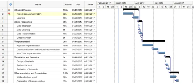
1.4.2 Gantt chart
Figure 2: Gantt chart
1.4.3 Tasks and dependencies Project planning
In this first phase, the scope and the objectives of the project are defined.
In the Project Planning phase there are two tasks. In theory they are independent, but due to the large workload that the Project Management (GEP) task creates, the two tasks are done mostly one after the other.
Data preparation
In this phase of the project the datasets will be prepared for their future usage. The tasks that constitute this stage have to be performed in order, as they are dependent on each other.
In the first one, the different datasets will be merged into a single dataset. In the Data Cleaning and Data Transformation tasks, the dataset will be processed in order to fill the missing values, smooth noisy data, identify or remove outliers, and resolve inconsistencies. In the last task of this stage, the dataset will be divided into the Training dataset, the Evaluation dataset and the Testing dataset.
Implementation
In this development phase there are three main tasks. They have been planned to be done sequentially, one after the other.
This stage represents the main part of the development process, and during this period all the features of the final system will be implemented.
Validation and evaluation
In this stage the tests will be designed and performed in order to check that the system works as expected.
With the help of the tests’ results, the system performance will be evaluated and analysed. Documentation and presentation
This last stage of the project consists in writing the final report and preparing the oral presentation of the project, that will be done in front of a tribunal that will evaluate the work done.
1.5
Resources
1.5.1 Human resourcesThe only human resource that will be available during the project will be a single developer, that will perform the different roles necessary to complete the project. The dedication to the project will be around 30 hours per week. This is an approximation that can change depending on the workload of each week.
1.5.2 Material resources
During the project, different resources will be used.
1. Custom Desktop Computer (CPU i7 2700k, GPU nvidia GeForce GTX 560 Ti, 8GB RAM). Hardware tool used in the development of the project. The code of the project will be written with it, as well as reports.
2. Lenovo ThinkPad t450s laptop. It will be used with the same purposes as the Desktop compter.
3. Git and GitHub. Version control system for tracking changes in the project codes. GitHub online services will be used.
4. Sublime Text 2. Text editor used to write the code of the project.
5. Apache Spark. Open-source cluster-computing framework in which the system will be developed.
6. Gantter. Online tool to make Gantt Charts.
7. Asana. Online tool to keep track of the project state.
1.6
Risks and alternatives
The project is expected to be presented between the 26th and the 30th of June. Due to the fact that there will be a lot of work involving technologies yet to learn for the developer, it is possible that the development will take more time than estimated and the project won’t be finished in time. In case this scenario happens, the project would be presented in October. The stage where more problems are bound to happen is the implementation phase, as the developer has to learn and use new technologies.
Another possible problem that can arise during the development of the project is the lack of any physical infrastructure to test the system. In this case, virtualisation should be considered to evaluate the system. This should be considered when analysing the performance results. In the most optimistic scenario the project would be finished sooner than expected. In this case, there would be the possibility to talk with the director to discuss new features for the project.
A more realistic estimation would be finishing the project with all its planned features just in time, or even having to extend it four months and finishing it on October.
The worst case scenario would be having to extend the duration of the project and having to reduce the expected features of the system in order to finish the development in time.
1.7
Economical management of the project
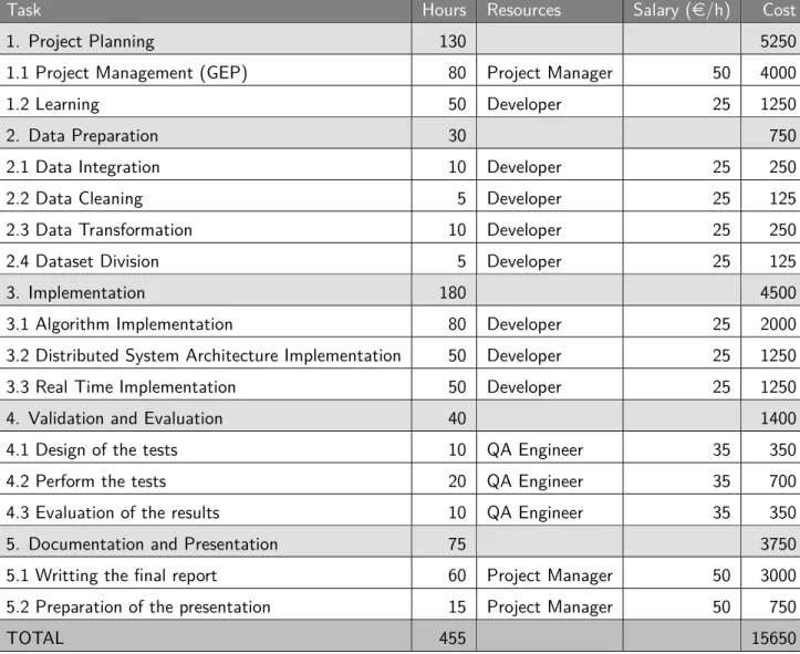
1.7.1 Estimation of costsHuman resources costs
Only one worker will be working on this project, and he will have to perform all the tasks. However, to estimate human costs, it has been taken into consideration that the different roles performed entail different costs. The cost/hour of a project manager should be around 50e/hour. Contrarily, the developer’s wage should be around 25e/hour. The salary of the engineer is estimated to be 35e/hour.
Task Hours Resources Salary (e/h) Cost
1. Project Planning 130 5250
1.1 Project Management (GEP) 80 Project Manager 50 4000
1.2 Learning 50 Developer 25 1250
2. Data Preparation 30 750
2.1 Data Integration 10 Developer 25 250
2.2 Data Cleaning 5 Developer 25 125
2.3 Data Transformation 10 Developer 25 250
2.4 Dataset Division 5 Developer 25 125
3. Implementation 180 4500
3.1 Algorithm Implementation 80 Developer 25 2000
3.2 Distributed System Architecture Implementation 50 Developer 25 1250
3.3 Real Time Implementation 50 Developer 25 1250
4. Validation and Evaluation 40 1400
4.1 Design of the tests 10 QA Engineer 35 350
4.2 Perform the tests 20 QA Engineer 35 700
4.3 Evaluation of the results 10 QA Engineer 35 350
5. Documentation and Presentation 75 3750
5.1 Writting the final report 60 Project Manager 50 3000
5.2 Preparation of the presentation 15 Project Manager 50 750
TOTAL 455 15650
Table 2: Direct costs by activity according to the Gantt Chart
Task Hours Salary (e/h) Estimated Cost (e
Project manager 155 50 7750
Developer 260 25 6500
QA Engineer 40 35 1400
TOTAL 15650
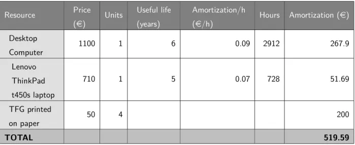
Material resources costs
In this section the costs of the material resources have been calculated.
It has been considered that the desktop computer will be used for 80% of the hours, and the laptop for the remaining 20%.
To calculate the amortization, it has been considered that a year has 250 laborable days, and each laborable day has 8 hours of worktime.
Finally I have included the cost of printing the TFG. The price is estimated to be around 50e per copy. Four copies will be needed: three for each member of the tribunal and one for the director of the project.
The material costs are equally distributed among the different tasks of the project.
Resource Price (e) Units Useful life (years) Amortization/h (e/h) Hours Amortization (e) Desktop Computer 1100 1 6 0.09 2912 267.9 Lenovo ThinkPad t450s laptop 710 1 5 0.07 728 51.69 TFG printed on paper 50 4 200 TOTAL 519.59
Table 4: Indirect costs for material resources
Indirect costs
In this section all the indirect costs will be specified. The cost of the electricity, water, Internet and workplace will be my monthly housing costs, as my home will be the place where the project will be developed most of the time.
As well as with the material costs, the indirect costs are equally distributed among the different tasks of the project.
Product Price (e/month) Estimated Cost (e Internet 20 80 Workplace 375 1500 Electricity bill 37.5 150 Water bill 20 80 T-jove 1 zona 35 140 TOTAL 1950
Table 5: General indirect costs
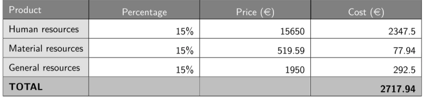
Cost contingency
The following costs will cover any possible problem that increases the real cost of the project. A percentage of 15% will be reserved for this purpose.
Product Percentage Price (e) Cost (e)
Human resources 15% 15650 2347.5
Material resources 15% 519.59 77.94
General resources 15% 1950 292.5
TOTAL 2717.94
Table 6: Cost contingency table
Unforeseen events
In this section possible unexpected events are taken into consideration:
1. Desktop computer failure. In case of failure of the desktop computer, it will have to be repaired or substituted for a new one. Due to the time constrains of the project, the best option would be to buy a new computer. In this case, 1100ewould be added to the cost of the project. However, the possibility of this failure happening is very low (we decide it is around 5% ).
2. In case of a failure in the laptop, the same scenario would take place, increasing the final cost in 710e.
Product Probability Units Price (e) Cost (e)
Desktop computer failure 5% 1 1100 55
Laptop failure 5% 1 710 35.5
TOTAL 90.5
Table 7: Unforeseen events costs.
Final Cost
The final cost of the project is shown in the table below.
Concept Cost (e) Human resources 15650 Material resources 519.59 Indirect costs 1950 Cost contingency 2717.94 Unforeseen events 90.5 TOTAL 20928.03
Table 8: Final cost of the project
In this calculation the costs of the taxes have been omitted. They should be taken into consideration as they might increase significantly the cost of the project.
1.7.2 Control management
There are very few factors that can be controlled in this project, as the material resources were bought time ago, and the indirect costs will exist even if nothing is developed. The only thing that can be controlled are human resources.
In case unexpected incidents occur and the project has to be extended four months, the cost would increase 1950 euros from the indirect general costs, and an unkown amount from the human resources costs, as more hours of work would be needed to end the project .
At the end of each phase of the project, the number of hours dedicated to its comple-tion will be computed and compared with the estimated hours, in order to control possible
deviations.
1.8
Sustainability
1.8.1 Economic dimensionIn the cost study carried out previously, it has been shown that most of the costs of the project come from the human resources expenses. The remaining costs are inevitable, and would exist even if there wasn’t any project in development. This low production and development costs make the project economically viable.
The strength of this project lies in the savings that this product would have for ISPs and MNOs, and the ability to create personal internet plans that it would give them. It would also be an economic benefit for companies and organizations that use this product to gain visibility in their networks.
1.8.2 Social Dimension
The social dimension of this project is very limited, and probably it won’t improve anybody’s life quality.
However, a positive social aspect of this project that might happen, is that thanks to the ISPs and MNOs being able to create and promote new and personalized services, prices could drop and make everybody able to afford an Internet plan.
A negative aspect of this project might be the loss of privacy, as this product will increase network visibility for network managers. Despite the sensation of privacy loss, this is a relatively insignificant problem, as network users will still be anonymous and only the type of traffic they are generating will be known.
1.8.3 Environmental dimension
Zero material resources have been specifically bought for this project. All the resources used where bought time ago for other purposes and will continue to be used after the end of this project, so no waste and pollution have been generated for the developement of this project. Although the enviromental impact of this project is very small, in the real implementation of the final product there will be a server or a network of servers always working, analysing the network traffic sent to them.
1.8.4 Sustainability Matrix
In the following table the sustainability of the project is evaluated. Environmental, economic and social categories have a score between 0 and 10, and the global score is between 0 and 30.
Sustainability Environmental Economic Social Total
Score 3 10 4 17
Apache Spark Framework
Apache Spark[8] is a general-purpose cluster computing system. The Spark project was born in 2009 at UC Berkeley’s AMPLab and made open source in 2010 under the BSD license. Later, in 2013, it was donated to the Apache Software Foundation, which changed its license to Apache 2.0.
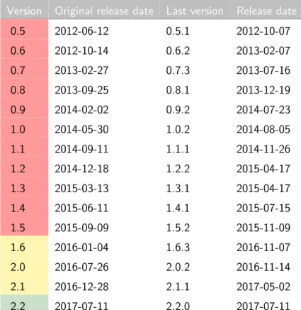
Version Original release date Last version Release date
0.5 2012-06-12 0.5.1 2012-10-07 0.6 2012-10-14 0.6.2 2013-02-07 0.7 2013-02-27 0.7.3 2013-07-16 0.8 2013-09-25 0.8.1 2013-12-19 0.9 2014-02-02 0.9.2 2014-07-23 1.0 2014-05-30 1.0.2 2014-08-05 1.1 2014-09-11 1.1.1 2014-11-26 1.2 2014-12-18 1.2.2 2015-04-17 1.3 2015-03-13 1.3.1 2015-04-17 1.4 2015-06-11 1.4.1 2015-07-15 1.5 2015-09-09 1.5.2 2015-11-09 1.6 2016-01-04 1.6.3 2016-11-07 2.0 2016-07-26 2.0.2 2016-11-14 2.1 2016-12-28 2.1.1 2017-05-02 2.2 2017-07-11 2.2.0 2017-07-11
Table 10: Spark versions. Legend
Old version
Older version, still supported
Latest version
In 2015 Spark had more than 1000 contributors, making it one of the most active projects of the Apache Software Foundation.
It provides high-level APIs in Java, Scala, Python and R, and can be integrated with Hadoop and can process existing Hadoop HDFS data.
In the big data indusitry there was the need for a general purpose cluster computing tool that solved the existing tools’ limitations. Hadoop MapReduced could only perform batch processing, Apache Storm could only perform stream processing, Apache Impala could only perform interactive processing, and Neo4j could only perform graph processing.
Apache Spark provided real-time stream processing, interactive processing, graph processing, and very fast in-memory batch processing.
Figure 3: Logistic regression in Hadoop and Spark.
Source: https://spark.apache.org/
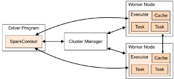
When a Spark application is excuted, the first step is to create the SparkContext object. This element is a logic connection with the cluster. This element is usually created within the main function, that is executed by the Spark Driver.
The Spark Driver is the program that declares the transformations and actions on the RDDs and submits such requests to the master. Its location is independent of the master and slaves.
The DAG Scheduler is the high-level scheduling layer that implements stage-oriented schedul-ing. It divides each job in different stages and computes DAG (Direct Acyclic Graph) with these stages. It also keeps track of which RDDs and stage outputs are materialized, and finds a schedule to run the job.
In addition to creating a DAG of stages, the DAG Scheduler also determines the best locations to run each task on, based on the current cache status. Furthermore, it handles failure.
Once the DAG Scheduler has sent the Direct Acyclic Graph to the Cluster Manager, the later creates tasks out of it and submits them to the workers, coordinating the different job stages. The workers are where the tasks are actually executed.
Figure 4: Spark cluster mode overview.
Source: http://spark.apache.org/docs/latest/img/cluster-overview.png
2.1
RDDs
The Resilient Distributed Dataset (RDD) is the fundamental data unit in Apache Spark. An RDD is an immutable distributed collection of elements of data, partitioned across nodes in a cluster that can be operated in parallel. RDDs can’t be changed, but new RDDs can be generated by transforming existing ones.
Each dataset in RDD is divided into logical partitions, which may be computed on different nodes of the cluster.
RDDs are fault tolerant. That means that in case of losing data in a calculation of an RDD, it can be recalculated from the original data. This is possible because RDDs are only readable. The system saves all the operations that the RDDs go through, and in case data needs to be recovered, the operations can be applied again to the original data.
RDDs are distributed in the different cluster nodes. Using the operation RDD.partition the granularity of the data can be configured. There are two types of basic operations: transformations and actions. The transformations create a new RDD from a set of data or
from another RDD. The actions calculate a result based on the data of one or more RDDs. Below are the most commonly used operations on RDDs, both transformations and actions. The complete list of operations can be dound in the programming guide published by Apache Spark1.
Transformation Description
map(func)
Returns a new distributed dataset, formed by passing each element of the source through a function func.
filter(func)
Returns a new dataset formed by selecting those elements of the source on which func returns true.
flatMap(func)
Similar to map, but each input item can be mapped to 0 or more output items (so func should return a Seq rather than a single item). union(otherDataset)
Returns a new dataset that contains the union of the elements in the source dataset and the argument.
intersection(otherDataset)
Returns a new RDD that contains the intersection of elements in the source dataset and the argument.
distinct([numTasks]) Returns a new dataset that contains the distinct elements of the source dataset.
join(otherDataset, [numTasks])
When called on datasets of type (K, V) and (K, W), returns a dataset of (K, (V, W)) pairs with all pairs of elements for each key. Outer joins are supported through leftOuterJoin, rightOuterJoin, and fullOuterJoin.
Table 11: RDD transformations
Source: http://spark.apache.org/docs/2.1.1/programming-guide.html
Spark uses a lazy evaluation approach. This means Spark does not evaluate each transfor-mation on the data right away, the execution will not start until an action is triggered. The transformations are added to the DAG, and only when the Driver requests some data, the DAG actually gets executed.
Some advantages of lazy evaluation are increased manageability, less computation time and 1
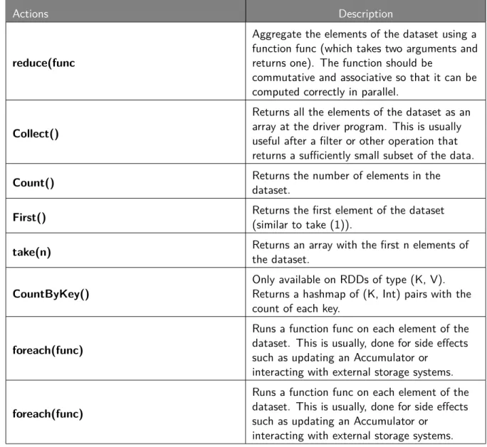
Actions Description
reduce(func
Aggregate the elements of the dataset using a function func (which takes two arguments and returns one). The function should be
commutative and associative so that it can be computed correctly in parallel.
Collect()
Returns all the elements of the dataset as an array at the driver program. This is usually useful after a filter or other operation that returns a sufficiently small subset of the data.
Count() Returns the number of elements in the
dataset.
First() Returns the first element of the dataset(similar to take (1)). take(n) Returns an array with the first n elements of
the dataset. CountByKey()
Only available on RDDs of type (K, V). Returns a hashmap of (K, Int) pairs with the count of each key.
foreach(func)
Runs a function func on each element of the dataset. This is usually, done for side effects such as updating an Accumulator or
interacting with external storage systems. foreach(func)
Runs a function func on each element of the dataset. This is usually, done for side effects such as updating an Accumulator or
interacting with external storage systems.
Table 12: RDD actions
Source: http://spark.apache.org/docs/2.1.1/programming-guide.html increased speed, reduced complexity and optimized excution.
With lazy evaluation, Apache Spark programs can be organized into smaller operations. It reduces the number of passes on data by grouping operations. Since only necessary values get computed, the trip between the driver and the cluster is saved, speeding up the process.
Figure 5: Space Efficiency: Datasets vs RDDs.
Source: https://databricks.com/blog/2016/07/14/a-tale-of-three-apache-spark-apis-rdds-dataframes-and-datasets. html
After Spark 2.0, RDDs are replaced by Dataset, which is strongly-typed like an RDD, but with richer optimizations under the hood. The RDD interface is still supported, however, is highly recommend to switch to use Dataset, which has better performance than RDD.
2.2
Datasets and dataframes
A Dataset is a collection of data distributed over different cluster nodes. Datasets were introduced in Spark 1.6 and provided the benefits of RDDS, like strong typing and the ability to use lambda functions, with the benefits of Sparks SQL’s optimized execution engine. ADataFrameis a Dataset organized into named columns. Conceptually, it is equivalent to a table in a relation database or a data frame in python, but with better optimizations under the hood.
2.3
Spark Components
Spark Core is the underlying general execution engine for the Spark platform. It comes with a set of high-livel libraries that provided increased functionalities, like support for SQL, streaming data and machine learning. These libraries can be combined to create complex workflows.
Next, the different modules that create the Apache Spark Ecosystem will be explained.
Figure 6: The Spark Platform.
Source: https://jaceklaskowski.gitbooks.io/mastering-apache-spark/ spark-overview.html
2.3.1 Spark Streaming
Spark Streaming[9] is an extension of the Spark core. It is an stream processing engine that enables high-throughput, scalable and fault-tolerant processing of live data streams.
To ingest data in the system many sources can be used, like Flume, Kafka, Kinesis or TCP sockets. This data can then be processed using algorithms and high level functions, like map,
reduce and join. You can apply Spark’s machine learning and graph processing algorithms on these data streams. After the data has been processed, it can be sent out to filesystems, live dashboards and databases.
Figure 7: Streaming architecture.
Source: https://spark.apache.org/docs/latest/streaming-programming-guide.html Internally, Spark Streaming ingests live input data streams divided into mini batches. RDD transformations are applied to the batches by the Spark engine to generate the final result.
Figure 8: Spark Streaming flow of data.
Source: https://spark.apache.org/docs/latest/streaming-programming-guide.html This structure allows the same code to be used for offline data processing and live stream analytics. This comes at the price of having a latency equal to the duration of the batch.
Discretized Streams
Discretized Streams, also known as Dstreams, are an abstraction of a continous flow of data provided by Spark Streaming. DStreams are actually series of RDDs, each one containing data from an specific time interval.
Figure 9: DStreams internal structure.
Source: https://spark.apache.org/docs/latest/streaming-programming-guide.html The operations on a DStream are internally applied to all the RDDs that compose the stream. Spark Streaming has two categories of streaming sources built-in.
• Basic sources: Sources directly available in the StreamingContext API, like sockets and filesystems.
• Advanced sources: Sources available through external libraries, like Flume, Kafka and Kinesis.
Applications that use Spark Streaming need to be run on more than one core, or thread when running locally, as one core is needed to run the receiver, and another to process the received data.
Structured Streaming
Structured Streaming[10] was introduced in Spark 2.0. It is a collection of additions to Spark Streaming rather than a huge change to Spark itself. This leads to a new stream processing model that is very similar to a batch processing model.
The main idea behing Structured Streaming is to have a table that is constantly having new entries added to it. This new model, while being more optimized, has a resemblance to the old batch processing model.
Figure 10: Input Table in Structure Streaming.
Source: https://spark.apache.org/docs/latest/structured-streaming-programming-guide. html
Every data element arrived on the stream is like a new row being appended to the table. A transformation on the input table will generate the “Result Table”. Every trigger inter-val(for example, every 1 second), new rows are appended to the input table, which results in updates in the Result Table.
There are different modes to decide what gets pushed out to the external storage:
• Complete Mode: The entire table with the processed data is pushed out to the external storage. Is the storage connector that has to decide if it writes the entire table or filters it.
• Append Mode: Only the new rows appended in the table since the last trigger are pushed out to the external storage. This mode is only useful when the existing rows on the results table are not expected to change.
• Update Mode: The rows that were updated since the last trigger will be written to the external storage. Note that this is different from the Complete Mode in that this mode only outputs the rows that have changed since the last trigger.
2.3.2 Spark SQL
Spark SQL is a Spark module that introduces a new data abstraction, SchemaRDD, that provides support for semi-structured and sructured data. One of the main characteristic is that it provides relational processing with Spark functional programming. Unlike the basic Spark RDD API, the interfaces of Spark SQL provides Spark with more information about the structure of the data and the computation when are being performed. Internally, this extra information is used to perform extra optimizations.
Figure 11: Architecture of Spark SQL.
Source: https://www.edureka.co/blog/spark-sql-tutorial/
The main capabilities of Spark SQL in terms of using structured and semi-structured data are:
1. Provides a DataFrame abstraction in Python, Scala and Java. This integration simpli-fies working with structured datasets and makes it easy to run SQL queries alongside complex analytic algorithms.
2. Unifies Data Acces by reading and writting data from a variety of structured formats as JSON, Hive Tables and Parquet (providing a single interface for an efficient work.) 3. Allows to query data from other structured formats as JSON, HIve Tables, etc; using
SQL. 2.3.3 GraphX
GraphX is a Spark’s API extension for graphs and graph-parallel computation. It includes ready-to-use graph algorithms to simplify analytics tasks. Some of this algorithms are
PageR-ank, Connected Components and Triangle Counting. 2.3.4 MLlib
MLlib[7] is Spark’s machine learning library. It helps deploy applications that use machine learning algorithms in a practical and easy way, taking advantage of the scalability the cluster offers.
Machine learning is the field of computer science that has the goal to make computers learn without being explicitly programmed.
It provides high level tools, such as:
• Machine learning algorithms for classification, regression and clustering.
• Featurization: attem iribute selection, dimensionality reduction, transformation and feature extraction.
• ML Pipelines.
• Persistence: loading and saving models, Pipelines and algorithms.
The available algorithms and functionalities can be consulted at the Machine Learning Library (MLlib) Guide2.
With the realease of Spark 2.0, the RDD-based APIs in the spark.mllib package have entered maintenance mode. Now, the primary Machine Learning API for Spark is the DataFrame-based API in the spark.ml package.
2.3.5 Cluster Deployment
To take profit of the full potential of Apache Spark it needs to be run on a cluster. To do so, a cluster manager and a distributed storage system are needed.
Spark can use a wide variety of distributed storage systems, including Hadoop Distributed File System (HDFS), MapR File System (MapR-FS), Cassandra, OpenStack Swift, Amazon S3 or Kudu. It also allows a custom solution to be implemented.
Spark can connecto to several types of cluster managers. The cluster manager is responsible allocating resources for applications across the cluster. Once the cluster is up and running, Spark acquires executors on the cluster nodes, which are processes that run computations and
2
store data. When the executors are ready, it sends the code to them. Finally, SparkContext sends different tasks to the executors.
This architecture provides isolation to the applications, making them independent at schedul-ing and execution level. However this makes sharschedul-ing data between applications impossible without writing it to an external storage system. Spark is indifferent to the cluster manager, as long as it an acquire executors, and these can communicate with each other.
The latest Spark release (version 2.2.0) suports three different cluster managers: 1. Standalone: a simple cluster manager included with Spark.
2. Apache Mesos: an open-source cluster manager developed ad University of California, Berkeley.
3. Hadoop YARN: the resource manager in Hadoop 2.
4. Kubernetes: Kubernetes is an open-source platform for providing container-centric infrastructure. Currently the support is only experimental.
By default, standalone scheduling clusters are resilient to Worker failures (insofar as Spark itself is resilient to losing work by moving it to other workers). However, the scheduler uses a Master to make scheduling decisions, and this (by default) creates a single point of failure: if the Master crashes, no new applications can be created. In order to circumvent this, we have two high availability schemes, detailed below.
Standby masters with ZooKeeper ZooKeeper is a service that using it allows to provide a leader election and state storage mantainig the configuration information, naming, providing distributed syncronization and group services. With this service you can launch multiple masters in your cluster by being connected to the same ZooKeeper’s instance; one of them will be elected as ”leader” and the other will remain in standby mode. In case that the ”leader” dies, another master will be choosen, recovering the old master’s state, and the resume scheduling. This entire recovering process, since the first moment that the first leader goes down, should take beween one or two minutes. Note that the delay only affects to the programation of new applications, the applications that were already running during the failover remain unaffected.
Single-Node Recovery with Local File System The best way to go for the high availabil-ity of the production level is ZooKeeper. However. when the master crushes, there is enough registered information in the filesystem to be able to recovr the status of the master. There is enough state written in the directory to recover the master process when the applications and workers are regustered.
Implementation
In this chapter, I provide details and explanations about the implementation of my project. The codes are available at https://github.com/marccode/tfg.
3.1
Project Structure
It was decided that the scope of the project wouldn’t include developing a connector to put real data from Cisco routers into Spark, so an instance generator was created, in order to simulate input data. It was programmed with Bash, and can be adjusted to send data at different rates of flows/second.
To ingest data directly into Spark, Apache Kafka has been used. It provides a distributed platform to stream data in real time, from any number of sources to any number of listeners, through any number of topics.
THeinstage generator outputs the simulated network traffic into a Kafka producer.
Our Apache Spark cluster uses a Kafka consumer to receive data from the producer. Once the network flows arrive at the Spark receiver running in a cluster node, they are divided into RDDs, each RDD containing data from a specific time window. These series of RDDs are feed into the Spark Mllib Pipeline containing the required preprocessing steps and the actual classifier model.
After being classified by the machine learning model, the data instances are saved into a MariaDB SQL Server. The database contains information about all the features of each flow, the result of its classification, and the date and time it was received by Spark.
This database can be queried by a live dashboard, which displays in real time the results of the classification of the incoming data instances in dynamic charts.
Figure 12: Architecture of project.
3.2
Dataset
The dataset used to train and evaluate teh developed system was provided by the director of the thesis[1]. It contains a vector of features of each traffic flow, along with the application that generated it. The vector consists of features obtained from the NetFlow feature in Cisco Routers. Netflow is a network protocol designed by Cisco Systems to collect network traffic going through an interface.
The datasets consisted originally of 7 different archives, collected at the UPC Gigabit acess link.
Each traffic set was registered at different hours, with the objective of collecting flows as much different as possible. For example, we can expect the networks at night to be full of backup applications traffic, or to collect more skype calls during the day than at night. Following the same logic, the traffic on the weekend won’t be the same as the traffic during a week day.
The days and hours were the datasets were collected can be seen on the table below. Once the traffic was captured, the flows had to be classified in order to obtain a trainning dataset and an evaluation dataset. This process was done with an automatic tool based on the L7-filter[5], as explained on [X: article del Pere]. As it is explained in the referred article, the accuracy of the tool was probably not as agood as a manual inspection. However, millions of flows had to be classified, thus it was impossible to do the classification manually. This stablished the ”base truth” upon which the classification of flows would be based.
Name Date Day Start Time Duration Packets Bytes
UPC-I 11-12-08 Thursday 10:00 15 minutes 95 M 53 G
UPC-II 11-12-08 Thursday 12:00 15 minutes 114 M 63 G
UPC-III 12-12-08 Friday 16:00 15 minutes 102 M 55 G
UPC-IV 12-12-08 Friday 18:30 15 minutes 90 M 48 G
UPC-V 21-12-08 Sunday 16:00 1 hour 167 M 123 G
UPC-VI 22-12-08 Monday 12:30 1 hour 345 M 256 G
UPC-VII 10-03-09 Tuesday 03:00 1 hour 114 M 78 G
Table 13: Information of the datasets
The dataset had 57 different classes and 32071325 instances. However, not all the flows were classified and some of them had an unknown origin/application. The 21057548 unkown instances were removed from dataset, leaving us with 11013777 instances.
0 1 2 3 4 5 6 7 radmin msnmessenger h323 httpcachemiss smtp battlefield2142 edonkey armagetron shoutcast soulseek mohaa vnc validcertssl quake-halflife jabber battlefield2 ftp socks sip whois bittorrent kugoo xboxlive worldofwarcraft ares dns httpaudio httpcachehit dhcp stun smb nbns rtsp http ventrilo skypeout ntp yahoo telnet pop3 ssl ssh pressplay httpvideo skypetoskype imap qq ident rlogin http-itunes freenet gnutella aim x11 lpd rtp 6 2,862 93 18,354 1.73·105 8 2.66·106 171 46 3,433 1,014 4 730 33,575 70 7 1,484 4,146 100 4 3.88·106 50 10 4 3,648 3.04·106 430 47,720 86 15,383 358 10,232 678 2.02·106 4 7.11·105 8.32·105 10 6 9,988 2.11·105 7,778 38 576 7.21·106 226 82,809 1,184 20 314 100 50,660 98 2,895 24 11,481 39
Next, each class of the dataset is briefly explained[5]: • radmin: Remote control software.
• msnmessenger: Instant messaging client.
• h323: Standard from the ITU Telecommunication Standardization Sector that defines the protocols to provide audio-visual communication sessions on any packet network. • httpcachemiss: Proxy Cache miss for HTTP.
• Smtp: Simple Mail Transfer Protocol.
• battlefield2142: Traffic generated by Battlefield 2142 online video game. • edonkey: Decentralized, server-based, peer-topeer file sharing network. • armagetron: Multiplayer game.
• shoutcast: Software for streaming media over the Internet. • soulseek: Peer-to-peer file sharing network and application.
• mohaa: Traffic generated by Medal of Honor: Allied Assault videogame. • vnc: Virtual Network Computing traffic.
• validcertssl: Valid certificate SSL. • quake-halflife: Half Life 1 engine games. • jabber: Open instant messenger protocol. • battlefield2: EA videogame Battelfield 2. • ftp: File Transfer Protocol.
• socks: Firewall traversal protocol. • sip: Session Initiaion Protocol.
• whois: Query/response protocol used for domain name info. • bittorrent: Peer-to-peer file sharing tool.
• kugoo: Chinese peer-to-peer program. • xboxlive: Console.
• worldofwarcraft: World of Warcraft online game. • ares: Peer-to-peer file sharing program.
• dns: Domain Name System. • httpaudio: Audio over HTTP.
• httpcachehit: Proxy Cache hit for HTTP. • dhcp: Dynamic Host Configuration Protocol. • stun: Simple Traversal of UDP through Nat.
• smb: Samba. Server Message Block. Microsoft Windows file sharing. • nbns: NetBIOS name service.
• rtsp: Real Time Streaming Protocol. • http: HyperText Transfer Protocol. • ventrilo: VoIP.
• skypeout: Skype to phone. • ntp: Network Time Protocol.
• yahoo: Yahoo messenger. Instant messenger protocol. • telnet: Insecure remote login.
• pop3: Post Office Protocol version 3. Application-layer Internet standard protocol used by local e-mail clients to retrieve e-mails form a remote server.
• ssl: Secure Socket Layer. • ssh: Secure Shell.
• pressplay: Legal music distribution site. • httpvideo: Video over HTTP.
• skypetoskype: Skype to Skype voice call.
• imap: Internet Message Access Protocol (E-mail). • qq: Chinese instant messenger protocol.
• ident: Identification Protocol. • rlogin: Remote login.
• http-itunes: iTunes traffic.
• freenet: Peer-to-peer platform for censorship-resistan communication. • gnutella: Peer-to-peer file sharing.
• aim: AOL instant messenger.
• x11: X Windows Version 11. Networked GUI system used in Unix. • lpd: Line Printer Daemon Protocol
• rtp: Real-time Transport Protocol.
With the dataset cleaned, some operations to enrich it have been carried out. For example, the duration of the flow has been obtained from the initial and final time and the average packet size of the flow has been computed.
All the fields of the feature vector can be seen at table14 on page43.
In order to have single dataset from which to obtain the training dataset and evaluation dataset all the datasets were merged in a single one. Next, to avoid problems with the date and time of creation of each flow when training the model, all the flows have been shuffled and randomly selected to constitute the two datasets.
No information about IP adresses is included nor used in this dataset. This can affect the overhall system classification performance negatively, however what could be seen at first as a limitation comes with two positives aspects: it makes the trained model less dependent on the network it has been trained on, and it doesn’t violate the privacy of the users of the networks were it is used, as it is not known which computers have created the flows.
Feature Description
protocol IP protocol value src port Source port of the flow dest port Destination port of the flow
packets Total number of packets in the flow bytes Flow length in bytes
start time Time stamp of the first packet of the flow end time Time stamp of the last packet of the flow. duration Duration of the flow in nanoseconds precision bytes per packet Average packet size of the flow
ToS Type of Service from the first packet
urg TCP flag ack TCP flag psh TCP flag rst TCP flag syn TCP flag fin TCP flag
Table 14: Description of the features of the dataset
3.3
Classification Model
For this work, three classifiers have been selected for its evaluation. Next, a brief description of each one is presented.
3.3.1 Studied Classifiers Naive Bayes
The Naive Bayes classifier is based on the Bayes Theorem and predits the outcome of a classification using the conditional a posteriori probability of a categorical class variable given independent predictor variables probabilities.
true in real-world escenarios. Decision Tree
Decision trees are supervised learning models used for classifcation and regression. They have a flowchart structure where each internal node represents an evaluation or test on an attribute and each branch represents the outcome of the evaluation. Finally, each leaf (final node) represents a class label.
To construct a decision tree all the features are considered and different split points are tested using a cost function. The split with the best cost is selected. Different algorithms use different metrics for evaluating the splits. This method is recursive, as the formed subtrees can be subdivided using the same technique.
In this work the decision tree that has been used is the famous C4.5, specifically its weka implementation J48.
K-nearest Neighbours
K-nearest neighbours is a classification algorithm that uses the class of the nearest neighbours of an instance to determine its class. In order to calculate which are the nearest neighbours, a distance concept has to be defined. This classifier has only one parameter, K, that specifies the number of neighbouring instances to be taken into consideration.
The main disavadvantage of this model is that it won’t perform well if the distance function is not correctly selected.
The implementation used is the one provided with the Weka software. 3.3.2 Classifier training and evaluation
Usually, 70% of the classified instances were used to train the model, leaving the remaining 30% for evaluation and testing. This was the traditional split of the dataset done in the majority of the machine learning projects, however there is no formal justification for it. In the particular case of this project, as millions of classified instances were available, there was no need to use a high percentage of the dataset to train the model. To decide how many instances were to be used for training purposes, a model was trained initially with 30% of the data (1717440 instances). Then, another model was trained with 10% less of instances. The performance metrics of the second model were the same as the first one, so another model
was trained with 10% less instances than the second model. This process was followed until the performance metrics of the model decreased.
This method helped to reduce overfitting, a phenomenon produced by the over specialisation of the model in a specific dataset.
Validation
In order to compare classifiers and decide which one is better we need stablish how we are going to evaluate them. After processing the testing dataset with a classifier we obtain a confusion matrix.
True Class
Total population valid not valid
valid True positive (Tp) False Positive (Fp) Predicted class
not valid False negative (Fn) True negative (Tn)
Table 15: Confusion matrix
Theconfusion matrix represents the intersection between the classifier results and the actual classes of the dataset. A classified data instance can be one of four types:
• True Positive (Tp): A positive element classified as positive. • True Negative (Tn): A negative element classified as negative. • False Positive (Fp): A negative element classified as positive. • False Negative (Fn): A positive element classified as negative.
From the confusion matrix we can obtain the metrics we will be using to evaluate the models. • Accuracy: Represents the proportion of correctly classified elements.
Accuracy= T p+T n
T p+F p+T n+F n
• Precision: Considering the elements classified as a certain class, the precision repre-sents the proportion of elements that are in fact from that class.
P recision= T p
• Recall: ARepresents the proportion of valid elements selected.
Recall= T p
T p+F n
• F-measure (F1): F-measure considers both the precision and the recall in a proportion that can be adjusted. In this project the same proportion has been used. This is called harmonic mean.
F−measure(F1) = 2∗P recision∗Recall P recison+Recall
Evaluation
The full confusion matrices are available at the appendix A. Naive Bayes
The software Weka has been used to evaluate this algorithm. As the results below show, it doesn’t perform well in this case.
Correctly Classified Instances15.7776% Incorrectly Classified Instances84.2224% Weighted Avg. TP Rate: 0.158 FP Rate: 0.039 Precision: 0.441 Recall: 0.158 F-Measure: 0.174 K-nearest Neighbours
The implementation of K-Nearest Neighbours of Weka Ibk has been used with a parameter k, neighbours to use, of 1. The results are shown below.
Correctly Classified Instances86.6485% Incorrectly Classified Instances13.3515% Weighted Avg. TP Rate: 0.866 FP Rate: 0.033 Precision: 0.859 Recall: 0.866 F-Measure: 0.861
Decision Tree
Decision Trees can create biased trees if some classes dominate, and therefore it is recom-mended to balance the dataset before training the decision tree.
In our case, eventhough the dataset has some imbalances, the classes with less weight have nearly no appearances at all compared to the other classes. Consequently, balancing the dataset will increase the accuracy and precision of the classifier on these classes, but this will have little effect on the total accuracy and precision, as instances of these classes won’t appear very often. This, however, will cause the global False Positive rate to increase, as more instance will be classified as if they were of these minoritary classes.
Correctly Classified Instances93.1931% Incorrectly Classified Instances6.8069% Weighted Avg. TP Rate: 0.932 FP Rate: 0.018 Precision: 0.929 Recall: 0.932 F-Measure: 0.930
After getting the results of the previous tests it was decided to use the Decision Tree clas-sifier, as it provided the best performance metris and it was known that it had the best computational cost.
3.3.3 Optimizations
After deciding which classifier to use a few changes were made to improve the system performance.
Optimization 1: PCA
The Principal Component Analysis (PCA) is a statistical procedure that uses an orthogonal transformation to convert a set of observations of possibly correlated variables into a set of values of linearly uncorrelated1.
Doing a Principal Compenent Analysis on the dataset we get the following results: 1
Ranked attributes:
0.6186 1 0.429protocol-0.429ack-0.429fin-0.429syn-0.426psh
0.4736 2 -0.654start time-0.653end time+0.281packets+0.243bytes+0.062bytes pkts 0.3417 3 -0.655bytes-0.63packets-0.268end time-0.268start time-0.153bytes pkts 0.2696 4 -0.71bytes pkts-0.589dest port+0.275tos+0.215src port+0.114packets 0.1982 5 -0.958tos-0.209dest port-0.192bytes pkts+0.031packets+0.024bytes 0.1304 6 -0.823src port-0.43dest port-0.329duration+0.102bytes pkts+0.081tos 0.0682 7 0.553bytes pkts-0.548dest port+0.501src port-0.373duration-0.052packets 0.0113 8 0.839duration+0.328bytes pkts-0.328dest port-0.114syn-0.114ack
If we now use the dataset obtained from the PCA to evaluate the classifier model we get the results shown below:
Correctly Classified Instances84.507% Incorrectly Classified Instances15.493% Weighted Avg. TP Rate: 0.845 FP Rate: 0.042 Precision: 0.837 Recall: 0.845 F-Measure: 0.840
As we can see, after applying the results of the Principal Component Analysis and reducing to eight the features used by the Decision Tree the results are slighty worse. Nonetheless, the results are still good, and if the performance of the system is low, PCA could be an interesting option, as it could help to process huge volums of data in real time by reducing the number of features, making the classifier simple, and thus reducing the computational cost.
Optimization 2: Dataset modifications
After observing the resuls of the classification model, some changes on the dataset classes can be purposed.
First of all, it has to be noted that this system’s goal would be to be a tool for network and system administrators to help classify the traffic on their networks. This can lead to diverse interpretations of what classes of traffic the system has to differentiate. The modifications shown below don’t diminish the information provided by this system to its users, but improves its performance.
In all the following tables the white rows are the results before the modification, and the grey rows the results after the modification.
Skype
The TP rate of skypeout is not very high because its instances usually are classified as bittorrent and edonkey. A possible reason for this is that skype uses a peer-to-peer protocol, as well as bittorrent and edonkey.
TP Rate FP Rate Precision Recall F-Measure Weighted Avg. 0.932 0.018 0.929 0.932 0.930
Skypeout 0.499 0.011 0.622 0.499 0.554
Skypetoskype 0.962 0.037 0.931 0.962 0.946
Skype 0.930 0.051 0.916 0.930 0.923
Weighted Avg. 0.935 0.024 0.934 0.935 0.934
Table 16: Skype Metrics
After the modification, the metrics of the new category skype are a bit lower than the ones that skypetoskype used to have, however they are still good results, and the new weighted average is higher than before. Moreover, there are more true positive instances of the new class skype than the sum of the true positive instances of the old skypeout and skypetoskype classes.
HTTP
All the metrics of the http-itunes and httpaudio classes were 0 because non of the instances were classified correctly. There were 3 instances of both http-itunes and httpaudio classes, and in both cases 2 of them were classified as http. The classifier also had problems separating httpcachemiss from httpcachehit, and both were also usually classified as http.
After the modification on the dataset all the metrics of the class http improve, and so does the weighted average.
Torrents
The biggest problem the classifier had with traffic generated by torrents applications was to differentiate it from skype traffic. This could be due to the fact that skype uses p2p to communicate, like torrents filesharing applications do.
In the confusion matrix we can see that the total instances of torrent applications’ flows classified as skype class where a total of 4982, but after the modification the misclasification were reduced to 4791 instances.
Games
TP Rate FP Rate Precision Recall F-Measure Weighted Avg. 0.932 0.018 0.929 0.932 0.930 http 0.954 0.010 0.913 0.954 0.933 httpcachemiss 0.455 0.000 0.568 0.455 0.505 httpcachehit 0.758 0.000 0.831 0.758 0.793 httpaudio 0.000 0.000 0.000 0.000 0.000 httpvideo 0.200 0.000 0.200 0.200 0.200 http-itunes 0.000 0.000 0.000 0.000 0.000 http 0.957 0.010 0.915 0.957 0.936 Weighted Avg. 0.935 0.024 0.935 0.935 0.935 Table 17: HTTP Metrics
because they nearly never appeared on the dataset. After the modification, the new cat-egory has lightly lower performance metrics than quake-halflife had. However we improve enormously the other game categories. In the confusion matrix can be seen how nearly all the instances of the games category are classified correctly.
TP Rate FP Rate Precision Recall F-Measure Weighted Avg. 0.932 0.018 0.929 0.932 0.930 edonkey 0.802 0.016 0.879 0.802 0.839 soulseek 0.742 0.000 0.767 0.742 0.754 bittorrent 0.974 0.008 0.966 0.974 0.970 kugoo 0.000 0.000 0.000 0.000 0.000 ares 0.813 0.000 0.867 0.813 0.839 gnutella 0.949 0.000 0.913 0.949 0.931 torrents 0.915 0.026 0.941 0.915 0.928 Weighted Avg. 0.939 0.028 0.940 0.939 0.939
Table 18: Torrents Metrics
3.4
Real-time Streaming
One of the initial requirements of the projecte was that it had to be able to process data in real time. To fulfill it, the module Spark Streaming has been used.
As it has been explained, Spark can take data into the system from a diverse range of systems. In this project two of the available options have been used. First, during the development phase, tcp sockets were used to ingest the data. A custom script was created in order to control the ammount of data sent to the Spark Streaming receiver.
Later in the implementation phase, it was decided to change the data ingestion mechanism in order to provide more reliability to the system. Apache Kafka was choosen.
3.4.1 Apache Kafka
Kafka[4] is a distributed streaming platform for moving data in real time. It works like a publish-subscribe system, and its architecture makes it fault tolerant and scalable.
Kafka stores messages that come from many processes calledproducers. Producers push the data into topics, which are simply a stream of messages. Another type of processes called consumers query Kafka and get the messages published to thetopics they are subscribed to.