Improving monsoon precipitation prediction using combined convolutional and long short term memory neural network

UC Irvine

UC Irvine Previously Published Works

Title

Improving Monsoon Precipitation Prediction Using Combined Convolutional and Long

Short Term Memory Neural Network

Permalink

https://escholarship.org/uc/item/899027nb

Journal

WATER, 11(5)

ISSN

2073-4441

Authors

Miao, Qinghua

Pan, Baoxiang

Wang, Hao

et al.

Publication Date

2019-05-01

DOI

10.3390/w11050977

License

https://creativecommons.org/licenses/by/4.0/ 4.0

Peer reviewed

eScholarship.org

Powered by the California Digital Library

Article

Improving Monsoon Precipitation Prediction Using

Combined Convolutional and Long Short Term

Memory Neural Network

Qinghua Miao1_{, Baoxiang Pan}2,_{*, Hao Wang}1,3_{, Kuolin Hsu}2_{and Soroosh Sorooshian}2 1 _{State Key Laboratory of Hydroscience and Engineering, Department of Hydraulic Engineering,}

Tsinghua University, Beijing 100084, China; [email protected] (Q.M.); [email protected] (H.W.)

2 _{Center for Hydrometeorology and Remote Sensing, University of California, Irvine, CA 92617, USA;} [email protected] (K.H.); [email protected] (S.S.)

3 _{Department of Water Resources, China Institute of Water Resources and Hydropower Research,} Beijing 100038, China

* Correspondence: [email protected]

Received: 1 April 2019; Accepted: 5 May 2019; Published: 9 May 2019 Abstract:Precipitation downscaling is widely employed for enhancing the resolution and accuracy of precipitation products from general circulation models (GCMs). In this study, we propose a novel statistical downscaling method to foster GCMs’ precipitation prediction resolution and accuracy for the monsoon region. We develop a deep neural network composed of a convolution and Long Short Term Memory (LSTM) recurrent module to estimate precipitation based on well-resolved atmospheric dynamical fields. The proposed model is compared against the GCM precipitation product and classical downscaling methods in the Xiangjiang River Basin in South China. Results show considerable improvement compared to the European Centre for Medium-Range Weather Forecasts (ECMWF)-Interim reanalysis precipitation. Also, the model outperforms benchmark downscaling approaches, including (1) quantile mapping, (2) the support vector machine, and (3) the convolutional neural network. To test the robustness of the model and its applicability in practical forecasting, we apply the trained network for precipitation prediction forced by retrospective forecasts from the ECMWF model. Compared to the ECMWF precipitation forecast, our model makes better use of the resolved dynamical field for more accurate precipitation prediction at lead times from 1 day up to 2 weeks. This superiority decreases with the forecast lead time, as the GCM’s skill in predicting atmospheric dynamics is diminished by the chaotic effect. Finally, we build a distributed hydrological model and force it with different sources of precipitation inputs. Hydrological simulation forced with the neural network precipitation estimation shows significant advantage over simulation forced with the original ERA-Interim precipitation (with NSE value increases from 0.06 to 0.64), and the performance is only slightly worse than the observed precipitation forced simulation (NSE=0.82). This further proves the value of the proposed downscaling method, and suggests its potential for hydrological forecasts.

Keywords: precipitation downscaling; convolutional neural networks; long short term memory networks; hydrological simulation

1. Introduction

Precipitation is a primary force in hydrological systems [1]. Obtaining accurate and reliable precipitation data at relevant spatial and temporal scales is crucial for efficient water resources management and timely warning of precipitation-related natural hazards, such as flood and

Water2019,11, 977 2 of 18

drought [2,3]. To sustain a reasonably long lead-time for the above-mentioned applications, it is imperative to employ precipitation prediction techniques.

For short-term range up to climate range, numerical weather/climate modeling is perhaps the only reliable tool for predictions. Through the past decades, numerical models have achieved impressive progress in predicting atmospheric dynamics and physics [4]. Here, dynamics refers to atmospheric state variables (i.e., density, pressure, temperature, and velocity) that are explicitly described by atmospheric primitive equations and resolved by numerical partial differential equation solvers, while physics refers to the unresolved processes that are diagnosed from the resolved variables based on empirical parameterization schemes. Precipitation results from complex processes that are mostly parameterized. Compared to a model’s relatively satisfactory skills in resolving atmospheric dynamics, the model’s precipitation estimation suffers from multiple sources of errors [5], and the skill has been described as “dreadful” [6]. The uncertainties for precipitation prediction generally stem from the following aspects: (1) a model’s dynamical forcings are of limited resolution for making detailed representation of cloud microphysics; (2) we usually do not have direct observation of the initial distribution state for cloud hydrometeors of liquid, solid, or mixed phases; (3) the evolution and interaction of precipitating cloud hydrometeors are not well described, due to our limited understanding or computation resources. A model’s deficiencies in each of the above aspects quickly reveal themselves in the precipitation product [5]. Many studies have revealed that the accuracy of the rainfall prediction in GCMs (such as ECMWF and National Centers for Environmental Prediction (NCEP)) is far from sufficient to be used directly in the East Asian monsoon region [7,8]. Besides the “dreadful” effect, the resolution of the

computing grids, is also usually too coarse for hydrological simulations [9–11].

To improve the precipitation estimations of GCMs, hydrologists have developed various downscaling methods, including dynamical downscaling and statistical downscaling [9,12–17]. Dynamical downscaling usually includes running a regional climate model with the initial and boundary conditions provided by GCMs. The massive computational cost and the requirement of local conditions has severely limited its application in many regions. Statistical downscaling establishes statistical links between large scale weather and local observation. Despite some limitations, such as the stationarity assumption in the predictor–predictand relationship and the requirement for long observation records, the statistical downscaling method is straightforward and computationally efficient. It can numerically simulate the physical process only based on historical data and does not require specialized knowledge, thus it can be easily applied to different regions [18].

There have been many statistical downscaling methods proposed by past researchers. The simplest form is linear regression, which estimates target predictand using an optimized linear combination of local circulation features [19–21]. The features are usually represented as the leading Principal Components (PC) of moisture, pressure, and wind field. While the leading PCs represent the inner linear structure of the circulation field at climate scale, they might not be directly related to the predictand at weather scale. For instance, frontal precipitation is closely related to its corresponding cyclone geometries, such as depression intensity, coverage, and distance. These geometries are highly varied from event to event, not all of them can be well illustrated through the leading eigenvectors of the circulation field.

Some other methods estimate precipitation based on non-linear features of the relevant circulation field, such as the self-Organizing Map (SOM) [22]. SOM clusters the synoptic circulation field into different categories, with each category defining a spatial rainfall pattern. However, a similar charge for principal component regression applies here as well, since these features are not designed based on predictor–predictand connection but the inner structure of the predictor, which does not necessarily relate to weather scale precipitation distribution.

Another category of machine learning algorithms uses kernel regression to implicitly transfer raw input data into feature space, from which the learning algorithm could better extract useful information for a given target. This is achieved through applying a kernel function to estimate two points’ distance in the feature space by transforming their dot-product in the input space. Kernel

trick allows customizing features toward a specific target by selecting kernel functions and their parameters. Relevant applications include kernel regression [23] and the support vector machine (SVM) [24–26]. The design of kernels relies heavily on the modeler’s prior knowledge. For the problem here, it is difficult to design kernel functions that explicitly consider the precipitation related influences of depression intensity, coverage, or distance for different cyclone events or convective activities.

The requirement for recognizing key circulation features of different appearances and positions led us to adopt deep Neural Networks. Artificial Neural Networks (ANN) have also been widely applied to precipitation downscaling problems in the past [20,27–29]. However, conventional ANNs tends to get trapped in poor local minima, and are relatively worse or no better than other downscaling methods. Recent progress in ANN such as Convolutional Neural Networks (CNNs) and recurrent neural networks (RNNs), have gained great success in many applications like speech recognition, visual object recognition, and object detection, etc. Some studies [30,31] have proved the effectiveness

of CNNs in precipitation downscaling in the United States. Shi et al. (2015) [32] proposed a new method for radar precipitation nowcasting by combining the CNNs with Long Short Term Memory Networks (LSTM).

Besides, instead of correcting biases for a numerical model’s precipitation estimations, many studies propose the prediction of rainfall based on model resolved circulation dynamics. This is motivated by the fact that, although the predictive skills for both precipitation and circulation dynamics diminish along the forecast lead time, the primitive variables are generally more reliable and sustain a longer usable forecast range. In past studies, many predictors have been used for precipitation downscaling, such as geopotential height [33], sea level pressure [34], geostrophic vorticity [35], or wind speed [36]. The choice of the predictors vary across different regions, characteristics of large-scale atmospheric circulation, seasonality, and geomorphology [37]. Susceptibility analyses might be conducted if necessary, using methods such as multivariate discriminant analysis or support vector machines [38,39].

In this study, we attempt to improve precipitation estimations using the state of art deep learning methods. CNNs and LSTM are two states of the art in deep learning. CNNs are good at dealing with spatially related data and LSTM is good at dealing with temporal signals. Both spatial and temporal characteristics of atmospheric circulation are very important for precipitation estimation. To take the advantages from both CNNs and LSTM, this study develops a deep neural network composed of convolution layers and the LSTM recurrent module to estimate precipitation based on well-resolved atmospheric dynamical fields. The review article by Amir et al. (2018) [18] shows that ANN and SVM are the two methods that are most widely used in hydrology; and the quantile mapping method is another relatively simple but popular statistical approach that has been successfully used in hydrologic studies (e.g., [40]). Thus these methods are also included as benchmarking.

After the Introduction, Section2presents the study area and datasets. Section3introduces the downscaling methods and hydrological model used in this study. The results of precipitation estimation as well as its performance evaluation are described in Section4. Finally, a brief summary and the major conclusions are provided in Section5.

2. Study Area and Datasets 2.1. Study Area

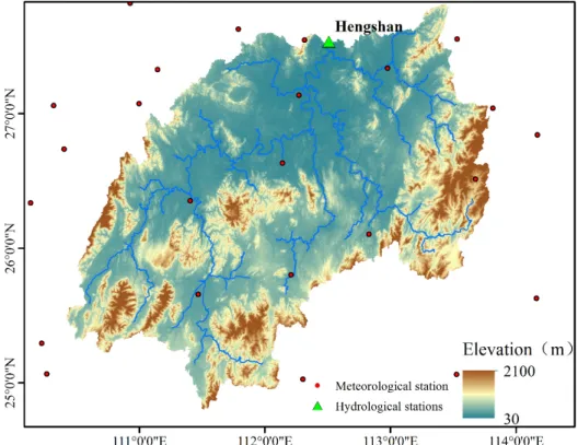
The Xiangjiang River, a tributary of the Yangtze River with a drainage area of 63,980 km2at the Hengshan hydrological station, was selected as the study area (see Figure1). This basin is located in the southeastern Hunan Province in South China and extends from longitudes of 109.27◦E to 114.99◦ E from latitudes of 23.98◦ N to 28.64◦ N. The climate of this region is humid subtropical monsoon, with a mean annual precipitation of approximately 1366 mm. The precipitation in this region exhibits high seasonal and inter-annual variability and mainly occurs between April and September. The annual average runoffdepth is approximately 822 mm. The area has complex topography, with elevations ranging from 30 m to 2097 m above sea level. The headwater regions are characterized by

Water2019,11, 977 4 of 18

steep mountain slopes and deep fluvial valleys and consequently suffer from flash flooding. The lower portion of the river flows through the floodplain where the outlet station Hengshan is located.

Water 2019, 11, x FOR PEER REVIEW 4 of 19

steep mountain slopes and deep fluvial valleys and consequently suffer from flash flooding. The lower portion of the river flows through the floodplain where the outlet station Hengshan is located.

Figure 1. Study basin and locations of the hydrological station and meteorological stations.

2.2. Datasets

Data used to train and validate the downscaling methods includes observed rainfall data and the predictor for precipitation estimation. The observation data is the China Gauge-Based Daily Precipitation Analysis product developed by the National Meteorological Information Center [41], with a temporal–spatial resolution of one day and 0.25°, and can be downloaded from the website (http://data.cma.cn). Products from the European Centre for Medium Range Weather Forecasts (ECMWF) Interim Reanalysis (ERA-Interim) [42] are selected as the predictors for precipitation estimation. It has a temporal-spatial resolution of one day and 0.75°. The potential predictor candidates used in this study include the following simulated atmospheric circulation variables: the mean sea level pressure (MLS), the total column water (TCW), the convective available potential energy (CAPE); and also the geo-potential height (GH), the U wind component (UW), the Vertical velocity (VV), the air temperature (T), potential vorticity (PV) at 500/700/850/925/1000 hpa. Detailed description of these variables can be found in the website (https://apps.ecmwf.int/codes/grib/param-db). The final predictors were determined through a trial and error method. Data from longitudes of 106° E to 125° E, and from latitudes of 20° N to 33° N are extracted for predictors. The range of predictand extends from 115° E to 120° E and from 24° N to 28° N.

To further validate the downscaling methods, we also used the ECMWF subseasonal to seasonal (S2S) prediction project database (hindcasts) [43], which contains the same predictors with ERA-Interim. The ECMWF hindcast model is initialized with realistic estimates of their observed states, hereafter iteratively predicts the weather for a preset extension without any boundary constraints. It restarts on every Monday and Thursday from 1995 to 2016 to forecast the next 46 days weather

Figure 1.Study basin and locations of the hydrological station and meteorological stations. 2.2. Datasets

Data used to train and validate the downscaling methods includes observed rainfall data and the predictor for precipitation estimation. The observation data is the China Gauge-Based Daily Precipitation Analysis product developed by the National Meteorological Information Center [41], with a temporal–spatial resolution of one day and 0.25◦, and can be downloaded from the website (http://data.cma.cn). Products from the European Centre for Medium Range Weather Forecasts (ECMWF) Interim Reanalysis (ERA-Interim) [42] are selected as the predictors for precipitation estimation. It has a temporal-spatial resolution of one day and 0.75◦. The potential predictor candidates used in this study include the following simulated atmospheric circulation variables: the mean sea level pressure (MLS), the total column water (TCW), the convective available potential energy (CAPE); and also the geo-potential height (GH), the U wind component (UW), the Vertical velocity (VV), the air temperature (T), potential vorticity (PV) at 500/700/850/925/1000 hpa. Detailed description of these variables can be found in the website (https://apps.ecmwf.int/codes/grib/param-db). The final predictors were determined through a trial and error method. Data from longitudes of 106◦E to 125◦E, and from latitudes of 20◦N to 33◦N are extracted for predictors. The range of predictand extends from 115◦E to 120◦E and from 24◦N to 28◦N.

To further validate the downscaling methods, we also used the ECMWF subseasonal to seasonal (S2S) prediction project database (hindcasts) [43], which contains the same predictors with ERA-Interim. The ECMWF hindcast model is initialized with realistic estimates of their observed states, hereafter iteratively predicts the weather for a preset extension without any boundary constraints. It restarts on every Monday and Thursday from 1995 to 2016 to forecast the next 46 days weather evolution, using 11 ensemble members. It is coupled with the ocean model but not the sea ice model. Together there were 1869 hindcast experiments during out validation period.

The other data used in this study include geographical information, which was used to build the distributed hydrological model; meteorological data, which were used as input data for the hydrological

model; and discharge data, which were used to calibrate and validate the hydrological model. Catchment topography is represented using a digital elevation model (DEM) with a spatial resolution of 90 m and the DEM data were downloaded from the SRTM Database (http://srtm.csi.cgiar.org). The soil map was obtained from the China Dataset of Soil Properties for Land Surface Modeling [44]. Land use/cover data were obtained from the Environmental and Ecological Science Data Center of West China (http://westdc.westgis.ac.cn/) and have a resolution of 100 m. To be consistent with the hydrological model (Section3.3), these data were resampled to obtain a resolution of 2 km using ArcGis software. Daily discharge data from the Hengshan hydrological station are available from 2007 to 2013 and were obtained from the Hydrological Year Book to calibrate and validate the hydrological model. Daily meteorological data were obtained from the China Administration of Meteorology and include precipitation, mean, maximum and minimum air temperatures, sunshine duration, wind speed, and relative humidity data. The meteorological data were used to estimate potential evaporation by using the Penman equation [45], which was also used in the hydrological model.

3. Methods

3.1. Downscaling Methods

3.1.1. Convolutional Neural Networks

The convolutional neural networks (CNNs) is a special type of Deep Neural Network. For a regular neural network, a statistical connection between the inputs and the outputs is constructed through hierarchical connected layers of neurons. Each neuron is a computing unit that receives some inputs, performs a dot product, and optionally follows a non-linear transformation. For supervised learning problems (i.e., classification and regression), a loss function is defined by comparing the network’s output estimations with observations. The network parameters are trained by minimizing the loss function using gradient descent, which is known as backpropagation training.

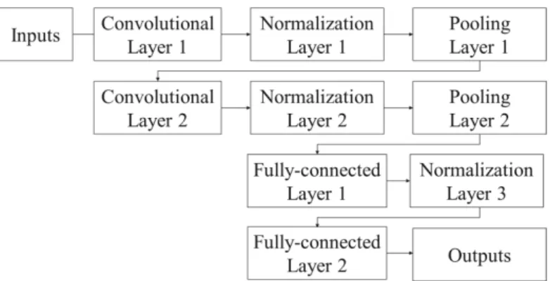
Different from the full-connected networks, CNNs involve two special matrix operators: a convolutional layer, and a pooling layer. Units in convolutional layers are only connected to specific local patches through a set of leant filters. In this way, it greatly reduces the number of parameters in the networks and allows the networks to be deeper and more efficient. Usually a non-linear function (such as rectified linear unit or hyberbolic tangent, etc.) is applied after the convolution operators [46]. Then the pooling layers are used to merge semantically similar local features into one [47]. This is due to the fact that the relative positions of features that make up the motifs may vary somewhat, thus coarsing the positions of each feature can help to detect reliably motifs. Typical pooling layers partition a feature map into a set of non-overlapping rectangles and output the maximum or the average value for each sub-region (Deep Learning Tutorials).

In addition, to reduce overfitting problems, dropout and batch-normalization methods are also adopted in this study. Dropout helps reduce overfitting by randomly setting some weight parameters or outputs of the hidden layers to zero with a predefined probability during the training process [48]. Batch-normalization alleviates internal covariate shift by normalizing layer inputs [49]. The CNNs are implemented in tensorflow [50] under python platform. Different predictors are fed as different

channels in the inputs. The Mean Square Error between the simulated and observed precipitation is used as loss function, which is defined as follows:

RMSE= v u t 1 N N X i=1 (Pi−Gi)2

wherePiandGidenote the predicted rainfall and observed gauge rainfall, respectively. The Adam

gradient-based optimizer is used to minimize the loss function. Figure2illustrates the architecture of the CNN networks used in this study.

Water2019,11, 977 6 of 18

Water 2019, 11, x FOR PEER REVIEW 6 of 19

where 𝑃 and 𝐺 denote the predicted rainfall and observed gauge rainfall, respectively. The Adam gradient-based optimizer is used to minimize the loss function. Figure 2 illustrates the architecture of the CNN networks used in this study.

Figure 2. Architecture of the CNN networks used in this study.

3.1.2. Combination of CNN and Long Short Term Memory Networks

The long short term memory networks (LSTM) [51] is a special type of recurrent neural network (RNN). RNNs contain a feedback connection that allows past information to affect the current output, thus is very effective for tasks involving sequential inputs [47]. As an extension of the conventional RNNs, LSTM introduces a special so-called memory cell, which acts like an accumulator to learn long-term dependency in a sequence, and make the optimization much easier. This cell is self-connected and will copy its own real-valued state and accumulate the external input. Simultaneously each cell is controlled by three multiplicative units—the input, output, and forget gates—to determine whether to forget past cell status or to deliver output to the last state, which allows the LSTM to store and access information over long periods. Following the work of Graves (2013) [52], the formulation are shown as follows:

(

)

(

)

(

)

(

)

( )

where 𝑖, 𝑓, 𝑜 represent the input, forget, and output gate; 𝑐 is the memory cell; 𝜎 is the logistic sigmoid function; h is a hidden vector; 𝑊 and 𝑏 are the gate matrix and bias terms.

To absorb advantages from both methods, we first use the convolutional layers to extract the spatial features of the raw input, and then feed them to the LSTM networks (hereinafter referred to as ConvLSTM). In this study, predictors from the past seven days are used to estimate daily rainfall. The structure of the convolutional layers are the same as previously mentioned and 400 hidden layers are set up in the LSTM, which is also implemented in the tensorflow [50] under the python platform. 3.1.3. Support Vector Machine

The Support Vector Machine (SVM) was first developed by Vapnik (1995) [53] for binary classification. The principle of the SVM algorithm is to find the optimal separation hyperplane

Figure 2.Architecture of the CNN networks used in this study. 3.1.2. Combination of CNN and Long Short Term Memory Networks

The long short term memory networks (LSTM) [51] is a special type of recurrent neural network (RNN). RNNs contain a feedback connection that allows past information to affect the current output, thus is very effective for tasks involving sequential inputs [47]. As an extension of the conventional RNNs, LSTM introduces a special so-called memory cell, which acts like an accumulator to learn long-term dependency in a sequence, and make the optimization much easier. This cell is self-connected and will copy its own real-valued state and accumulate the external input. Simultaneously each cell is controlled by three multiplicative units—the input, output, and forget gates—to determine whether to forget past cell status or to deliver output to the last state, which allows the LSTM to store and access information over long periods. Following the work of Graves (2013) [52], the formulation are shown as follows: it=σ(Wxixt+Whiht−₁+W_cic_t−₁+b_i) ft=σ Wx fxt+Wh fht−₁+W_{c f}c_t−₁+b_f ct= ftct−₁+ittanh(Wxcxt+Whcht−₁+bc) ot=σ(Wxoxt+Whoht−₁+W_coc_t+b_o) ht=ottanh(ct)

wherei,f,orepresent the input, forget, and output gate;cis the memory cell;σis the logistic sigmoid function; h is a hidden vector;Wandbare the gate matrix and bias terms.

To absorb advantages from both methods, we first use the convolutional layers to extract the spatial features of the raw input, and then feed them to the LSTM networks (hereinafter referred to as ConvLSTM). In this study, predictors from the past seven days are used to estimate daily rainfall. The structure of the convolutional layers are the same as previously mentioned and 400 hidden layers are set up in the LSTM, which is also implemented in the tensorflow [50] under the python platform. 3.1.3. Support Vector Machine

The Support Vector Machine (SVM) was first developed by Vapnik (1995) [53] for binary classification. The principle of the SVM algorithm is to find the optimal separation hyperplane between two classes by maximizing the boundary margin between the closest points of the class on the boundaries [54]. These points are called support vectors.

In SVM regression, the inputXis first mapped into a higher dimension feature space, and then a linear model can be constructed as follows [55,56]:

f(X,w) =X

j

wjgj(X) +b

wheregjdenotes a set of nonlinear transformations,wandbare model parameters to be calibrated.

Defining theε-insensitive loss functionL_ε(y,f(X,w))[53]: L_ε(y,f(X,w)) = ( 0 i f y−f(X,w) < ε y−f(X,w) −ε otherwise

Then the empirical risk can be calculated as: Remp(w) = 1 n n X i=1 Lε(yi,f(Xi,w))

Following Haykin (2003) regularization theory [57], by introducing (non-negative) slack variables ξi,ξ∗_ito measure the deviation of training samples outsideε-insensitive zone, the parameterswandb

are estimated by minimizing the cost function: min1₂k_wk_+CPN i=1 ξi+ξ ∗ i s.t.                yi−f(X,w)≤ε+ξi −_yi+f(X,w)≤ε₊ξ∗ i ξi≥0 ξ∗ i ≥0

where C is a positive real constant. This optimization problem can be solved by the method of Lagrangian multipliers [57]: w= N X i=1 αi−α∗_i g(Xi)

whereαiandα∗_i are the Lagrange multipliers, which are positive real constants.

In this study, the SVM model is implemented in Scikit-learn [58] under the python platform. The training of SVM includes selecting the kernel function, and determining the model parametersC and Gamma. These parameters are optimized through the grid search mechanism [59], whileC=10, Gamma=0.001 and the radial basis function are used in this study.

3.1.4. Quantile Mapping Method

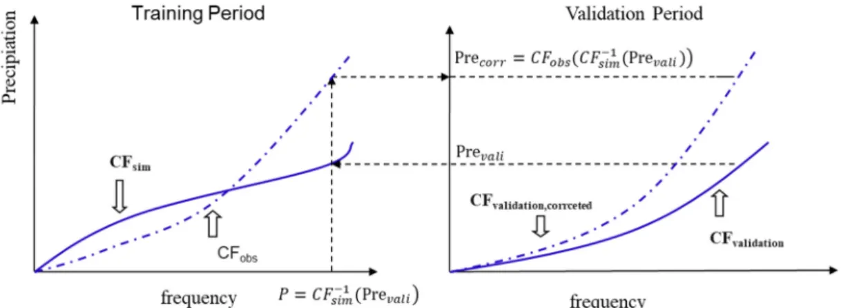
The quantile mapping (QM) method [60] is a relatively simple approach that has been successfully used in hydrologic studies (e.g., [40]). It uses the cumulative frequency curve of the observed precipitation to correct the simulated rainfall so that the corrected rainfall will have the same cumulative frequency curve as the observed one. Figure3illustrates how the quantile mapping method works. For each grid, calculate the cumulative frequency function of the simulated precipitation (CFsim(p)) and the observed precipitation (CFobs(p)), respectively. Then for a specific precipitation in

the validation period Prevali, we can calculate its frequency onCFsim(p)asCF−_sim1(Prevali). And then the

corresponding precipitation on the cumulative frequency function of the observed rainfall is just the corrected precipitation Precorr=CFobs(CF−_sim1(Prevali)).

Water 2019, 11, x FOR PEER REVIEW 8 of 19

1

(Pre )

sim vali

CF

. And then the corresponding precipitation on the cumulative frequency function of the observed rainfall is just the corrected precipitation

Pre

=

CF

(

CF

(Pre ))

Figure 3. Illustration of the quantile mapping method.

3.2. Statistical Evaluation Based on Gauge Rainfall Data

To qualitatively evaluate the downscaling methods, the following metrics were adopted: relative bias (RB), and the root mean square error (RMSE), which were used to show the error and bias of the simulated precipitation compared with the observed rainfall data; the correlation coefficient (CC), which aims to show the consistency between the predicted rainfall, and the observed rainfall. The metrics are calculated as follows:

1 1

(

)

RB

P

G

G

−

=





(

)

1

RMSE

P G

N

=



−

(

)(

)

CC

(

)

(

)

G G P P

G G

P P

−

−

=

−

−







where

P

G

3.3. Evaluation through Hydrological Modeling

Description of the Distributed Hydrological Model and Model Validation

The hydrological model used in this study is a distributed geomorphology-based hydrological model (GBHM) developed by Yang et al. [61–63]. In the GBHM, the study basin is divided into a number of sub-catchments linked by the river network and ordered by the Horton–Strahler scheme. Then, grids within a sub-catchment are grouped into several flow intervals according to the flow distance to the outlet. The runoff generated from the grids within a flow interval contributes to the

Water2019,11, 977 8 of 18

3.2. Statistical Evaluation Based on Gauge Rainfall Data

To qualitatively evaluate the downscaling methods, the following metrics were adopted: relative bias (RB), and the root mean square error (RMSE), which were used to show the error and bias of the simulated precipitation compared with the observed rainfall data; the correlation coefficient (CC), which aims to show the consistency between the predicted rainfall, and the observed rainfall. The metrics are calculated as follows:

RB= N P i=1 (Pi−Gi) T P t=1 Gi RMSE= v u t 1 N N X i=1 (Pi−Gi)2 CC= N P i=1 (Gi−G)(Pi−P) s N P i=1 (Gi−G) 2_PN i=1 (Pi−P) 2

wherePiandGidenote the predicted rainfall and observed gauge rainfall, respectively.

3.3. Evaluation through Hydrological Modeling

Description of the Distributed Hydrological Model and Model Validation

The hydrological model used in this study is a distributed geomorphology-based hydrological model (GBHM) developed by Yang et al. [61–63]. In the GBHM, the study basin is divided into a number of sub-catchments linked by the river network and ordered by the Horton–Strahler scheme. Then, grids within a sub-catchment are grouped into several flow intervals according to the flow distance to the outlet. The runoffgenerated from the grids within a flow interval contributes to the main stream with the same flow distance, and each grid is represented by a number of topographically similar “hillslope-valley” systems, which is the basic unit of the hydrological simulation [62,64].

The GBHM mainly consists of a hillslope module and a kinematic wave flow routing module [62,63]. In the hillslope module, the GBHM simulates the hydrological processes, including interception, evapotranspiration, infiltration, overland flow, unsaturated flow, and groundwater flow. Evapotranspiration is calculated as evaporation from water stored in the canopy, on the surface and from the soil surface in addition to transpiration from the root zone. The topsoil is divided into several layers according to depth, and the vertical soil water movement is described using the Richards equation. Overland flow is described using a one-dimensional kinematic wave equation. Subsurface flow along the hillslope occurs when the soil water content exceeds the field capacity. The groundwater aquifer (corresponding to each grid) is discretized and treated as an individual storage compartment. The water exchange between the groundwater and river channel is expected to be steady and is estimated using Darcy’s law [62]. Most model parameters are defined according to their physical meaning, either based on in situ measurements or regional databases. Only a few parameters must be calibrated, such as the hydraulic conductivity of the groundwater [65].

In this study, 170 sub-catchments are divided with a grid resolution of 2 km, as suggested by Yang et al. [66]. The GBHM simulates the hydrological processes at an hourly time step, and is calibrated for the period of 2007–2010, and is validated for the period of 2011–2013. The Nash and Sutcliffe

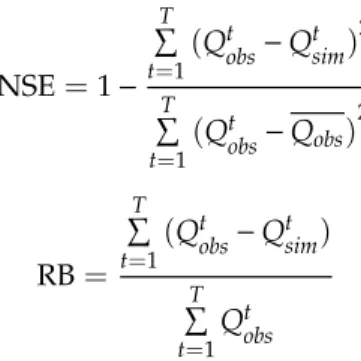
coefficient (NSE) and relative bias (RB) are adopted to evaluate the model performance and are defined as follows: NSE=1− T P t=1 (Qt obs−Q t sim) 2 T P t=1 (Qt_obs−_Qobs)2 RB= T P t=1 (Qt_obs−_Qt sim) T P t=1 Qt_obs whereQt obs andQ t

sim denote the observed and simulated discharge andQobs denotes the average

values of the observed discharges during the simulation periodT. Table1contains the calibration and validation results obtained from using gauge rainfall input data for the model. The NSE values for the calibration and validation period are greater than 0.8, and the absolute values of RB are less than 0.05, indicating that GBHM has good performance in the study basin.

Table 1. GBHM performance of daily discharge simulation during the calibration and validation periods at Hengshan Station.

Period NSE RB

Calibration period 0.89 0.04 Validation period 0.88 0.02

4. Results and Discussion

4.1. Precipitation Estimation Performance with Different Predictors

As mentioned before, predictors are very important for precipitation downscaling. So in this section, we designed four experiments to evaluate the forecast performance of different predictors. As listed in Table2, Experiment a represents the original ECMWF Interim precipitation; Experiment b uses the mean sea level pressure as predictor; Experiment c uses the geopotential height at 500/700/850/925/1000 hpa as predictors; Experiment d uses the geopotential height at 500/700/850/925/1000 hpa as well as the total column water as predictors; Experiment e uses all the circulation variables described in Section2.2

as predictors. Experiments b–e all use the CNN networks as downscaling method. Models were trained during the period from 1979 to 2002, and were validated from 2003 to 2016.

Table2lists the metrics of results of these experiments (note that the indexes are calculated for each grid respectively, and the average value for these indexes is shown in Table2; the same in Table3and Figure 6 and Figure 7). Precipitation estimations are plotted against observed ones in Figure4. Results of Experiment a show a relatively low correlation coefficient with the observed

data (with CC of 0.29) (for validation period, the same hereafter), along with an overestimation of the precipitation (with RB of 12.75%), the root-mean-square error is 11.48 mm/day. These metrics indicate a bad performance of the original ERA-interim rainfall. Results of Experiments b–e all outperform the original ERA-interim rainfall. Specifically, CC, RB, and RMSE values for Experiment b are 0.54, 5.53%, 8.86 mm/day. All metrics shows an improvement over Experiment a, but far from sufficient; and the scatter plots show that they severely underestimate the most high-intensity rainfall. The CC, RB, and RMSE values for Experiment c are 0.66, 4.08%, and 7.93, and the scatter plot indicates the model could well simulate the high-intensity rainfall. In Experiment d, the CC value further increases to 0.69. Experiment e gives the highest CC value of 0.72.

Overall, using as many of the meteorological variables as possible is conducive to improving the accuracy of downscaling rainfall. Among all meteorological variables, the geopotential height might

Water2019,11, 977 10 of 18

be the most useful one. Considering both the accuracy and complexity of the model, we suggest that the combination of geopotential height and total water vapor might be reasonable.

Table 2.Performance of downscaled precipitation using different predictors.

Exp Predictors Training Period (1979–2002) Validation Period (2003–2016) CC RB (%) RMSE (mm/day) CC RB (%) RMSE (mm/day) a p 0.31 16.53 11.16 0.29 12.75 11.48 b msl* 0.69 4.73 7.42 0.54 5.53 8.86 c gp* 0.79 4.46 6.2 0.66 4.08 7.93 d gp, tcw* 0.85 2.27 5.36 0.69 1.87 7.54

e gp, tcw, tem, uw, vw, cape,

vv, pv* 0.94 3.08 3.4 0.72 6.92 7.28

Note: p represents original ERA-interim precipitation; msl represents mean sea level pressure; gp represents geopotential height; tcw represents total column water; tem represents air temperature; cape represents convective available potential energy; uw represents u wind component; vw represents v wind component; vv represents vertical velocity; pv represents potential vorticity.

Water 2019, 11, x FOR PEER REVIEW 12 of 19

Figure 4. Scatterplots of estimated precipitation using different predictors against observed precipitation (daily scales): (a) Original ERA-Interim precipitation, (b) Sea level mean pressure, (c) Geopotential Height, (d) Geopotential Height filed and total column water, and (e) all circulation variables described in Section 2.2. And scatterplots of estimated precipitation using different downscaling methods against observed precipitation (daily scales): (f) Quantile mapping, (g) CNN networks, (h) SVM, and (i) ConvLSTM networks.

Figure 5. Similar to Figure 4h, but for area mean precipitation.

Figure 4.Scatterplots of estimated precipitation using different predictors against observed precipitation (daily scales): (a) Original ERA-Interim precipitation, (b) Sea level mean pressure, (c) Geopotential Height, (d) Geopotential Height filed and total column water, and (e) all circulation variables described in Section2.2. And scatterplots of estimated precipitation using different downscaling methods against observed precipitation (daily scales): (f) Quantile mapping, (g) CNN networks, (h) SVM, and (i) ConvLSTM networks.

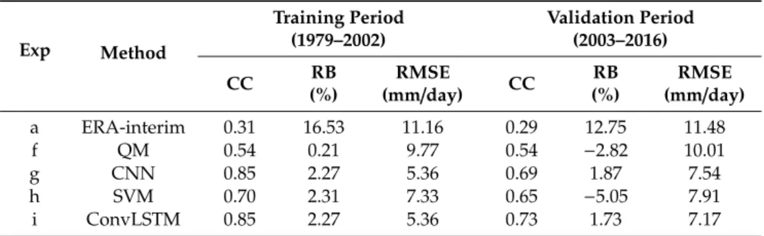
Table 3.Performance of downscaled precipitation using different downscaling methods. Exp Method Training Period (1979–2002) Validation Period (2003–2016) CC RB (%) RMSE (mm/day) CC RB (%) RMSE (mm/day) a ERA-interim 0.31 16.53 11.16 0.29 12.75 11.48 f QM 0.54 0.21 9.77 0.54 −_{2.82 10.01} g CNN 0.85 2.27 5.36 0.69 1.87 7.54 h SVM 0.70 2.31 7.33 0.65 −_{5.05 7.91} i ConvLSTM 0.85 2.27 5.36 0.73 1.73 7.17

4.2. Precipitation Estimation Performance of Different Methods

In this section, we compare the performance of different downscaling methods. The quantile mapping method, CNN networks, SVM, and ConvLSTM networks are used as downscaling methods for Experiments f–i, respectively. Experiment f uses ERA-interim precipitation as predictor, and Experiments g–i use geopotential height at 500/700/850/925/1000 hpa and total column water as predictors. For the quantile mapping method, regarding the inconsistency between the coarse input resolution (0.75◦) and the fine output resolution (0.25◦), we use the data in the coarse grid that covers the grid with fine resolution for calculation, to avoid additional errors caused by interpolating the coarse data to a fine resolution.

Metrics and scatter plots are shown in Table3and Figure4, respectively. Experiment f uses the traditional quantile mapping method. Its improvement upon the original ERA-interim precipitation is very limited. The CC value is only 0.54, and the RMSE value is 10.01 mm/day. However, it is worth mentioning that only in Experiment f, is the performance in the validation period comparable to the training period, which may be due to its simple model structure and fewer model parameters. While for other complex models, performance in the training period evidently exceeds the validation period, which reminds us that we should be cautious of whether the overfitting phenomena could lead to bad results in operation. Experiment g is the same as Experiment d in Section4.1, and we will not repeat it here. The SVM is used as the training method in Experiment h, the CC, RB and RMSE values for which are 0.65,−5.05%, and 7.91 mm/day. Although its evaluation indexes are comparable

to Experiment g, its scatter plots show that it could barely simulate the high intensity rainfall in the study area (although another study claims good performance of SVM in rainfall downscaling in other regions), which greatly limits its availability in hydrological simulation. Alternatively, if we change to draw the area mean precipitation, as shown in Figure5, the SVM methods can give reasonable results. The performance of Experiment i (using ConvLSTM) gives the best evaluation indexes, with CC value of 0.74, RB value of 1.73%, and RMSE value of 7.17 mm/day.Water 2019, 11, x FOR PEER REVIEW 13 of 19

Figure 6. Similar to Figure 5 (7), but for area mean precipitation.

Overall, the performance of these downscaling methods gradually increases according to the order quantile mapping, SVM, CNN networks, and ConvLSTM networks.

4.3. Application of Methods in Precipitation Forecast

To further estimate the robustness of the network, in this part we applied the trained network in precipitation forecasting based on the S2S ECMWF hindcast products. For simplicity, only the geopotential height at 500/700/850/925/1000 hpa and total water vapor content are used as the predictors in this section (Note that only geopotential is available in S2S ECMWF hindcasts, but it can be transferred to geopotential height by multiplying by a constant value of g = 9.80665), and ConvLSTM networks is used as the training model. For the 11 ensemble models, we first obtain the adjusted precipitation using the outputs of each model respectively, and then calculate their average as the final result.

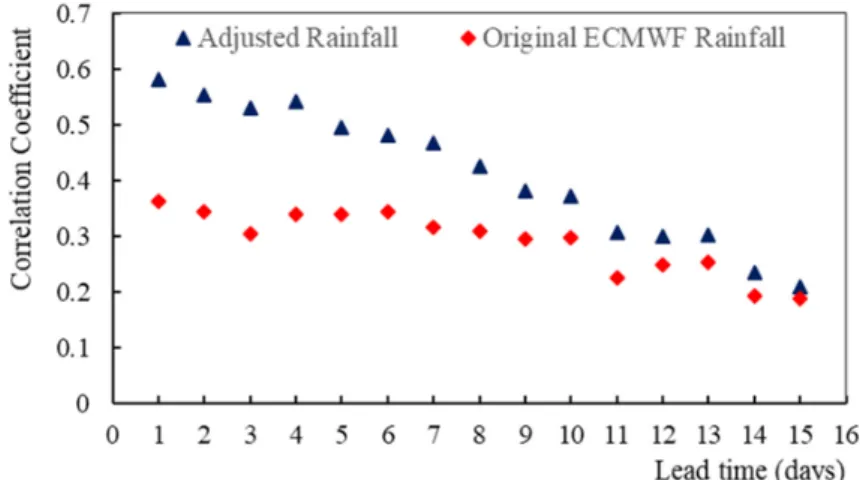
Figure 7 illustrates the predictive skill of S2S-ECMWF precipitation and the adjusted precipitation in the validation period as a function of forecast lead time. We can see that the performance of the corrected precipitation always outperforms the direct output of S2S-ECMWF. For the Day 1 forecast, the correlation coefficient between the corrected precipitation and the observed precipitation is 0.58, slightly lower than the result of Experiment 3 in Section 4.1 (with CC of 0.69), but significantly better than the S2S-ECMWF precipitation (with CC of 0.36). The difference of the correlation coefficient is 0.22. The CC values decrease sharply with the increase of lead time. For the Day 15 forecast, the CC value of the corrected precipitation and S2S ECMWF drop to 0.21 and 0.19 respectively, with a difference of only 0.02. In summary, the corrected precipitation is superior to the S2S-ECMWF throughout all the lead time, but the superiority gradually decreases with the increase of lead time.

Water2019,11, 977 12 of 18

Overall, the performance of these downscaling methods gradually increases according to the order quantile mapping, SVM, CNN networks, and ConvLSTM networks.

4.3. Application of Methods in Precipitation Forecast

To further estimate the robustness of the network, in this part we applied the trained network in precipitation forecasting based on the S2S ECMWF hindcast products. For simplicity, only the geopotential height at 500/700/850/925/1000 hpa and total water vapor content are used as the predictors in this section (Note that only geopotential is available in S2S ECMWF hindcasts, but it can be transferred to geopotential height by multiplying by a constant value of g=9.80665), and ConvLSTM networks is used as the training model. For the 11 ensemble models, we first obtain the adjusted precipitation using the outputs of each model respectively, and then calculate their average as the final result.

Figure6illustrates the predictive skill of S2S-ECMWF precipitation and the adjusted precipitation in the validation period as a function of forecast lead time. We can see that the performance of the corrected precipitation always outperforms the direct output of S2S-ECMWF. For the Day 1 forecast, the correlation coefficient between the corrected precipitation and the observed precipitation is 0.58, slightly lower than the result of Experiment d in Section4.1(with CC of 0.69), but significantly better than the S2S-ECMWF precipitation (with CC of 0.36). The difference of the correlation coefficient is 0.22. The CC values decrease sharply with the increase of lead time. For the Day 15 forecast, the CC value of the corrected precipitation and S2S ECMWF drop to 0.21 and 0.19 respectively, with a difference of only 0.02. In summary, the corrected precipitation is superior to the S2S-ECMWF throughout all the lead time, but the superiority gradually decreases with the increase of lead time.Water 2019, 11, x FOR PEER REVIEW 14 of 19

Figure 7. Predictive skill of S2S ECMWF precipitation and the corrected precipitation in the validation period as function of forecast lead time.

For the original ECMWF precipitation prediction, the uncertainty mainly comes from two sources. The first is dynamical deviation from the true atmosphere evolution, and the second is parameterization error due to the imperfect description of unresolved scale physical processes. Compared to the original ECMWF precipitation prediction, the downscaled precipitation can eliminate the parameterization error to some extent: on the one hand, it uses the observed precipitation, but the GCM is not calibrated locally; on the other hand, the straightforward ConvLSTM network uses a top-down parameterization paradigm, and might be more efficient when properly calibrated. When the lead time is short, both the two kinds of uncertainty sources cannot be ignored, thus performance of the ConvLSTM downscaling method presents a significant advantage over the S2S-ECMWF precipitation prediction. As the forecast lead time extends, the first kind of error (dynamical deviation) gradually dominates due to the chaotic effect, and thesuperiority of the ConvLSTM downscaling method gradually disappears.

Figure 8 shows the change of the related bias between S2S-ECMWF precipitation/the adjusted precipitation and the observed rainfall. We can see that although the correlation coefficient decreases significantly with the lead time, the relative biases of both adjusted rainfall and original ECMWF rainfall are generally more stable. The former approximately overestimates 5% rainfall, and the latter slightly overestimates 5% rainfall. This indicates that the improvement of systematic deviation of total rainfall will not disappear as lead time increases.

Figure 8. Relative bias of S2S ECMWF precipitation and the corrected precipitation in the validation period as function of forecast lead time.

Figure 6.Predictive skill of S2S ECMWF precipitation and the corrected precipitation in the validation period as function of forecast lead time.

For the original ECMWF precipitation prediction, the uncertainty mainly comes from two sources. The first is dynamical deviation from the true atmosphere evolution, and the second is parameterization error due to the imperfect description of unresolved scale physical processes. Compared to the original ECMWF precipitation prediction, the downscaled precipitation can eliminate the parameterization error to some extent: on the one hand, it uses the observed precipitation, but the GCM is not calibrated locally; on the other hand, the straightforward ConvLSTM network uses a top-down parameterization paradigm, and might be more efficient when properly calibrated. When the lead time is short, both the two kinds of uncertainty sources cannot be ignored, thus performance of the ConvLSTM downscaling method presents a significant advantage over the S2S-ECMWF precipitation prediction. As the forecast lead time extends, the first kind of error (dynamical deviation) gradually dominates due to the chaotic effect, and the superiority of the ConvLSTM downscaling method gradually disappears.

Water2019,11, 977 13 of 18

Figure7shows the change of the related bias between S2S-ECMWF precipitation/the adjusted

precipitation and the observed rainfall. We can see that although the correlation coefficient decreases significantly with the lead time, the relative biases of both adjusted rainfall and original ECMWF rainfall are generally more stable. The former approximately overestimates 5% rainfall, and the latter slightly overestimates 5% rainfall. This indicates that the improvement of systematic deviation of total rainfall will not disappear as lead time increases.

Figure 7. Predictive skill of S2S ECMWF precipitation and the corrected precipitation in the validation period as function of forecast lead time.

For the original ECMWF precipitation prediction, the uncertainty mainly comes from two sources. The first is dynamical deviation from the true atmosphere evolution, and the second is parameterization error due to the imperfect description of unresolved scale physical processes. Compared to the original ECMWF precipitation prediction, the downscaled precipitation can eliminate the parameterization error to some extent: on the one hand, it uses the observed precipitation, but the GCM is not calibrated locally; on the other hand, the straightforward ConvLSTM network uses a top-down parameterization paradigm, and might be more efficient when properly calibrated. When the lead time is short, both the two kinds of uncertainty sources cannot be ignored, thus performance of the ConvLSTM downscaling method presents a significant advantage over the S2S-ECMWF precipitation prediction. As the forecast lead time extends, the first kind of error (dynamical deviation) gradually dominates due to the chaotic effect, and thesuperiority of the ConvLSTM downscaling method gradually disappears.

Figure 8 shows the change of the related bias between S2S-ECMWF precipitation/the adjusted precipitation and the observed rainfall. We can see that although the correlation coefficient decreases significantly with the lead time, the relative biases of both adjusted rainfall and original ECMWF rainfall are generally more stable. The former approximately overestimates 5% rainfall, and the latter slightly overestimates 5% rainfall. This indicates that the improvement of systematic deviation of total rainfall will not disappear as lead time increases.

Figure 8. Relative bias of S2S ECMWF precipitation and the corrected precipitation in the validation period as function of forecast lead time.

Figure 7.Relative bias of S2S ECMWF precipitation and the corrected precipitation in the validation period as function of forecast lead time.

4.4. Application in Hydrological Simulation

After calibration and validation, the GBHM is run using the observed rainfall, the original ERA-interim rainfall and the downscaled rainfall (using geopotential height at 500/700/850/925/1000 hpa and total column water as predictors, ConvLSTM networks as downscale method, i.e., Experiment i in Section4.2) as input data, respectively. All simulations use the hydrological state at the end of 2010 as initial condition, which is obtained from continuous running of GBHM using gauge rainfall as input.

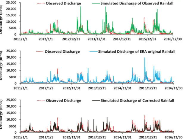
Table4gives the evaluation indexes and Figure8compares the streamflow simulation results using three sets of rainfall input at Hengshan station from 2011 to 2016, respectively. The simulation using observed rainfall data agrees well with the observed discharge, with NSE value of 0.82 and RB value of 7%. However, the original ERA-interim rainfall forced simulation is almost completely useless, with an NSE value of 0.06. It severely overestimates most flood peaks as shown in Figure8, and overestimate 24% of the total runoff. The simulation using the adjusted rainfall provides a reasonable result, with NSE value of 0.64 and RB value of –10%. It is close to the observed rainfall forced simulation, and far better than the original ERA-interim rainfall forced simulation. Hydrological systems are non-linear systems, uncertainties in precipitation inputs may be magnified when transferred to runoff, which makes the correction of the raw predicted rainfall more necessary.

Table 4.Performance of simulations with different precipitation forcing.

Precipitation Inputs NSE RB (%)

Observed Precipitation 0.82 7

Original ERA-interim Precipitation 0.06 24 Corrected Precipitation 0.64 −₁₀

Water2019,11, 977 14 of 18

Water 2019, 11, x FOR PEER REVIEW 15 of 19

4.4. Application in Hydrological Simulation

After calibration and validation, the GBHM is run using the observed rainfall, the original ERA-interim rainfall and the downscaled rainfall (using geopotential height at 500/700/850/925/1000 hpa and total column water as predictors, ConvLSTM networks as downscale method, i.e., Experiment 8 in Section 4.2) as input data, respectively. All simulations use the hydrological state at the end of 2010 as initial condition, which is obtained from continuous running of GBHM using gauge rainfall as input.

Table 4 gives the evaluation indexes and Figure 9 compares the streamflow simulation results using three sets of rainfall input at Hengshan station from 2011 to 2016, respectively. The simulation using observed rainfall data agrees well with the observed discharge, with NSE value of 0.82 and RB value of 7%. However, the original ERA-interim rainfall forced simulation is almost completely useless, with an NSE value of 0.06. It severely overestimates most flood peaks as shown in Figure 8, and overestimate 24% of the total runoff. The simulation using the adjusted rainfall provides a reasonable result, with NSE value of 0.64 and RB value of –10%. It is close to the observed rainfall forced simulation, and far better than the original ERA-interim rainfall forced simulation. Hydrological systems are non-linear systems, uncertainties in precipitation inputs may be magnified when transferred to runoff, which makes the correction of the raw predicted rainfall more necessary.

Table 4. Performance of simulations with different precipitation forcing.

Precipitation Inputs NSE RB (%)

Observed Precipitation 0.82 7

Original ERA-interim Precipitation 0.06 24

Corrected Precipitation 0.64 −10

Figure 9. Comparison of the hydrographs at Hengshan station among the observation (reference), observed precipitation-driven simulation, ERA-interim precipitation-driven simulation, and corrected precipitation-driven simulation.

Figure 8. Comparison of the hydrographs at Hengshan station among the observation (reference), observed precipitation-driven simulation, ERA-interim precipitation-driven simulation, and corrected precipitation-driven simulation.

5. Summary and Conclusions

In this study, we proposed a new method for precipitation downscaling by combining CNN and LSTM, based on model resolved circulation dynamics. This method was tested for precipitation estimation or prediction in the Xiangjiang River Basin in south China, which is located in the East Asian monsoon region. The results show that this method has advantages over the traditional quantile mapping method or SVM based method. The downscaled rainfall was further evaluated through a distributed hydrological model. The major conclusions can be summarized as follows:

1. Four experiments using different circulation predictors were designed to test the effectiveness of those predictors. Results show that using as many meteorological variables as possible is conducive to improving the rainfall estimation while using mean sea level alone can only provide limited improvement. Among all the meteorological variables, the geopotential height might be the most important one. Considering both the accuracy and complexity of the model, we suggest that the combination of geopotential height and total water vapor might be reasonable.

2. Another four experiments were designed to compare the different performance of the Quantile Mapping method, SVM, CNN networks, and ConvLSTM networks. Precipitation estimated by ConvLSTM networks gave the best performance (with highest correlation coefficient of 0.73), along with CNN, SVM, and the Quantile Mapping method, with correlation coefficient of 0.69, 0.65, 0.54 respectively. We also found that the method based on SVM could not predict very high intensity rainfall.

3. The trained ConvLSTM networks were applied to S2S-ECMWF hindcast datasets to further test their robustness. We found the corrected precipitation was superior to the original S2S-ECMWF precipitation all the time, but the superiority (in terms of correlation coefficient) gradually

decreased with the increase of the lead time. We think the improvement mainly comes from the use of observed data and the effective networks, which can reduce the parameterization error. However, when the lead time extends, the parameterization error becomes subordinate. Thus the superiority of the proposed method gradually fades away. However, the improvement for systematic deviation always holds for all lead times.

4. Different rainfall inputs are fed into the distributed hydrological model. The original EAR-Interim rainfall shows little usage in hydrological simulation with an NSE of 0.06 and RB of 24%, while the corrected rainfall forced simulation improves the NSE to 0.64 and reduces RB to−_{10%, which}

is comparable to the simulation forced by the observed rainfall. This further proves the value of the proposed method.

Author Contributions:Conceptualization, Q.M. and B.P.; methodology, Q.M.; software, Q.M.; validation, Q.M.; formal analysis, Q.M. and B.P.; investigation, Q.M.; resources, Q.M.; data curation, Q.M.; writing—original draft preparation, Q.M.; writing—review and editing, Q.M. and B.P.; visualization, Q.M.; supervision, H.W., K.S. and S.S.

Funding:This work was financially supported by the National Natural Science Foundation of China (project No. 41661144031), DoE CERC-WET award (DoE prime award DE-IA0000018), and the China Scholarship Council. Acknowledgments: The authors want to thank Yang Dawen for providing the data and guiding the buildup of GBHM.

Conflicts of Interest:The authors declare no conflict of interest. References

1. Nijssen, B.; Lettenmaier, D.P. Effect of precipitation sampling error on simulated hydrological fluxes and states: Anticipating the Global Precipitation Measurement satellites.J. Geophys. Res. Biogeosci. 2004,

109, 02103. [CrossRef]

2. Panagoulia, D.; Dimou, G. Sensitivity of flood events to global climate change.J. Hydrol.1997,191, 208–222. [CrossRef]

3. Panagoulia, D.; Dimou, G. Definitions and effects of droughts. In Proceedings of the Conference on Mediterranean Water Policy: Building on Existing Experience, Mediterranean Water Network, Valencia, Spain, 16 April 1998; General Lecture, Invited Presentation, ResearchGate: Berlin/Heidelberg, Germany, 1998. 4. Bauer, P.; Thorpe, A.; Brunet, G. The quiet revolution of numerical weather prediction.Nature2015,525,

47–55. [CrossRef]

5. Tapiador, F.J.; Roca, R.; Del Genio, A.; Dewitte, B.; Petersen, W.; Zhang, F. Is precipitation a good metric for model performance?Bull. Am. Meteorol. Soc.2019,100, 223–233. [CrossRef]

6. Stephens, G.L.; L’Ecuyer, T.; Forbes, R.; Gettelmen, A.; Golaz, J.-C.; Bodas-Salcedo, A.; Suzuki, K.; Gabriel, P.; Haynes, J. Dreary state of precipitation in global models.J. Geophys. Res. Atmos.2010,115, D24211. [CrossRef] 7. Kang, I.-S.; Jin, K.; Wang, B.; Lau, K.-M.; Shukla, J.; Krishnamurthy, V.; Schubert, S.; Wailser, D.; Stern, W.; Kitoh, A.; et al. Intercomparison of the climatological variations of Asian summer monsoon precipitation simulated by 10 GCMs.Clim. Dyn.2002,19, 383–395.

8. Wang, B.; Kang, I.-S.; Lee, J.-Y. Ensemble Simulations of Asian—Australian Monsoon Variability by 11 AGCMs*.J. Clim.2004,17, 803–818. [CrossRef]

9. Xu, C.-Y. From GCMs to river flow: A review of downscaling methods and hydrologic modelling approaches.

Prog. Phys. Geogr. Earth1999,23, 229–249. [CrossRef]

10. Ghosh, S. SVM-PGSL coupled approach for statistical downscaling to predict rainfall from GCM output.

J. Geophys. Res. Biogeosci.2010,115, D22102. [CrossRef]

11. Meehl, G.A.; Stocker, T.F.; Collins, W.D.; Friedlingstein, P.; Gaye, T.; Gregory, J.M.; Kitoh, A.; Knutti, R.; Murphy, J.M.; Noda, A.; et al.Climate Change 2007: The Physical Science Basis. Contribution of Working Group I to the Fourth Assessment Report of the Intergovernmental Panel on Climate Change, Chap. Global Climate Projections; Cambridge University Press: Cambridge, UK; New York, NY, USA, 2007.

12. Benestad, R. Novel methods for inferring future changes in extreme rainfall over Northern Europe.Clim. Res.

Water2019,11, 977 16 of 18

13. Benestad, R.E.; Haugen, J.E. On complex extremes: Flood hazards and combined high spring-time precipitation and temperature in Norway.Clim. Chang.2007,85, 381–406. [CrossRef]

14. Christensen, J.H.; Machenhauer, B.; Jones, R.G.; Schär, C.; Ruti, P.M.; Castro, M.; Visconti, G. Validation of present-day regional climate simulations over Europe: LAM simulations with observed boundary conditions.

Clim. Dyn.1997,13, 489–506. [CrossRef]

15. Hanssen-Bauer, I.; Achberger, C.; Benestad, R.E.; Chen, D.; Forland, E.J. Statistical downscaling of climate scenarios over Scandinavia.Clim. Res.2005,29, 255–268. [CrossRef]

16. Prudhomme, C.; Reynard, N.; Crooks, S. Downscaling of global climate models for flood frequency analysis: Where are we now?Hydrol. Process.2002,16, 1137–1150. [CrossRef]

17. Panagoulia, D.; Bárdossy, A.; Lourmas, G. Multivariate stochastic downscaling models generating precipitation and temperature scenarios of climate change based on atmospheric circulation.Glob. Nest J.

2008,10, 263–272.

18. Mosavi, A.; Ozturk, P.; Chau, K. Flood Prediction Using Machine Learning Models: Literature Review.Water

2018,10, 1536. [CrossRef]

19. Murphy, J. Predictions of climate change over Europe using statistical and dynamical downscaling techniques.

Int. J. Clim.2000,20, 489–501. [CrossRef]

20. Schoof, J.T.; Pryor, S. Downscaling temperature and precipitation: A comparison of regression-based methods and artificial neural networks.Int. J. Clim.2001,21, 773–790. [CrossRef]

21. Li, Y.; Smith, I. A Statistical Downscaling Model for Southern Australia Winter Rainfall.J. Clim. 2009,22, 1142–1158. [CrossRef]

22. Hope, P.K. Projected future changes in synoptic systems influencing southwest Western Australia.Clim. Dyn.

2006,26, 765–780. [CrossRef]

23. Kannan, S.; Ghosh, S. A nonparametric kernel regression model for downscaling multisite daily precipitation in the Mahanadi basin.Water Resour. Res.2013,49, 1360–1385. [CrossRef]

24. Tripathi, S.; Srinivas, V.; Nanjundiah, R.S. Downscaling of precipitation for climate change scenarios: A support vector machine approach.J. Hydrol.2006,330, 621–640. [CrossRef]

25. Pan, B.; Cong, Z. Information Analysis of Catchment Hydrologic Patterns across Temporal Scales.

Adv. Meteorol.2016,2016, 1–11. [CrossRef]

26. Anandhi, A.; Srinivas, V.V.; Nanjundiah, R.S.; Kumar, D.N. Downscaling precipitation to river basin in India for IPCC SRES scenarios using support vector machine.Int. J. Clim.2008,28, 401–420. [CrossRef]

27. Guhathakurta, P. Long lead monsoon rainfall prediction for meteorological sub-divisions of India using deterministic artificial neural network model.Theor. Appl. Clim.2008,101, 93–108. [CrossRef]

28. Taylor, J.W. A quantile regression neural network approach to estimating the conditional density of multi-period returns.J. Forecast.2000,19, 299–311. [CrossRef]

29. Norton, C.W.; Chu, P.-S.; Schroeder, T.A. Projecting changes in future heavy rainfall events for Oahu, Hawaii: A statistical downscaling approach.J. Geophys. Res. Atmos.2011,116, D17110. [CrossRef]

30. Vandal, T.; Kodra, E.; Ganguly, S.; Michaelis, A.; Nemani, R.; Ganguly, A.R. DeepSD: Generating High Resolution Climate Change Projections through Single Image Super-Resolution. In Proceedings of the 23rd ACM SIGKDD International Conference on Knowledge Discovery and Data Mining, Halifax, NS, Canada, 13–17 August 2017; pp. 1663–1672.

31. Pan, B.; Hsu, K.; AghaKouchak, A.; Sorooshian, S. Improving Precipitation Estimation Using Convolutional Neural Network.Water Resour. Res.2019,55, 2301–2321. [CrossRef]

32. Shi, X.; Chen, Z.; Wang, H.; Yeung, D.-Y.; Wong, W.; Woo, W. Convolutional LSTM Network: A machine learning approach for precipitation nowcasting.Int. Conf. Neural Inf. Process. Syst.2015. [CrossRef] 33. Kidson, J.W.; Thompson, C.S. A Comparison of Statistical and Model-Based Downscaling Techniques for

Estimating Local Climate Variations.J. Clim.1998,11, 735–753. [CrossRef]

34. Cavazos, T. Large-Scale Circulation Anomalies Conducive to Extreme Precipitation Events and Derivation of Daily Rainfall in Northeastern Mexico and Southeastern Texas.J. Clim.1999,12, 1506–1523. [CrossRef] 35. Wilby, R.; Wigley, T. Precipitation predictors for downscaling: Observed and general circulation model

relationships.Int. J. Clim.2000,20, 641–661. [CrossRef]

36. Murphy, J. An Evaluation of Statistical and Dynamical Techniques for Downscaling Local Climate.J. Clim.

37. Anandhi, A.; Srinivas, V.V.; Kumar, D.N.; Nanjundiah, R.S. Role of predictors in downscaling surface temperature to river basin in India for IPCC SRES scenarios using support vector machine.Int. J. Climatol.

2009,29, 583–603. [CrossRef]

38. Choubin, B.; Moradi, E.; Golshan, M.; Adamowski, J.; Sajedi-Hosseini, F.; Mosavi, A. An ensemble prediction of flood susceptibility using multivariate discriminant analysis, classification and regression trees, and support vector machines.Sci. Total Environ.2019,651, 2087–2096. [CrossRef]

39. Khosravi, K.; Pham, B.T.; Chapi, K.; Shirzadi, A.; Shahabi, H.; Revhaug, I.; Prakash, I.; Bui, D.T. A comparative assessment of decision trees algorithms for flash flood susceptibility modeling at Haraz watershed, northern Iran.Sci. Total. Environ.2018,627, 744–755. [CrossRef] [PubMed]

40. Boé, J.; Terray, L.; Habets, F.; Martin, E. Statistical and dynamical downscaling of the Seine basin climate for hydro-meteorological studies.Int. J. Climatol.2007,27, 1643–1655. [CrossRef]

41. Shen, Y.; Xiong, A. Validation and comparison of a new gauge-based precipitation analysis over mainland China.Int. J. Climatol.2016,36, 252–265. [CrossRef]

42. Dee, D.P.; Uppala, S.M.; Simmons, A.J.; Berrisford, P.; Poli, P.; Kobayashi, S.; Andrae, U.; Balmaseda, M.A.; Balsamo, G.; Bauer, P.; et al. The ERA-Interim reanalysis: Configuration and performance of the data assimilation system.Q. J. R. Meteorol. Soc.2011,137, 553–597. [CrossRef]

43. Vitart, F.; Ardilouze, C.; Bonet, A.; Brookshaw, A.; Chen, M.; Codorean, C.; Déqué, M.; Ferranti, L.; Fucile, E.; Fuentes, M.; et al. The Subseasonal to Seasonal (S2S) Prediction Project Database.Am. Meteorol. Soc.2017,

98, 163–173. [CrossRef]

44. Dai, Y.; Shangguan, W.; Duan, Q.; Liu, B.; Fu, S.; Niu, G. Development of a China Dataset of Soil Hydraulic Parameters Using Pedotransfer Functions for Land Surface Modeling.J. Hydrometeorol.2013,14, 869–887. [CrossRef]

45. Penman, H.L. Natural evaporation from open water, bare soil and grass.Proc. R. Soc. Lond. Ser. A Math. Phys. Sci.1948,193, 120–145.

46. Krizhevsky, A.; Sutskever, I.; Hinton, G.E. ImageNet classification with deep convolutional neural networks.

Int. Conf. Neural Inf. Process. Syst.2012,25. [CrossRef]

47. Lecun, Y.; Bengio, Y.; Hinton, G. Deep learning.Nature2015,521, 436–444. [CrossRef] [PubMed]

48. Hinton, G.E.; Srivastava, N.; Krizhevsky, A.; Sutskever, I.; Salakhutdinov, R.R. Improving Neural Networks by Preventing Co-Adaptation of Feature Detectors. Available online:https://arxiv.org/pdf/1207.0580v1.pdf (accessed on 3 July 2012).

49. Loffe, S.; Szegedy, C. Batch Normalization: Accelerating Deep Network Training by Reducing Internal Covariate Shift. Available online:https://arxiv.org/pdf/1502.03167.pdf(accessed on 2 March 2015).

50. Abadi, M.; Agarwal, A.; Barham, P.; Brevdo, E.; Chen, Z.; Citro, C.; Corrado, G.S.; Davis, A.; Dean, J.; Devin, M.; et al. TensorFlow: Large-Scale Machine Learning on Heterogeneous Distributed Systems. Available online:http://download.tensorflow.org/paper/whitepaper2015.pdf(accessed on 9 November 2015). 51. Hochreiter, S.; Schmidhuber, J. Long Short-Term Memory.Neural Comput.1997,9, 1735–1780. [CrossRef] 52. Graves, A. Generating Sequences with Recurrent Neural Networks. Available online:https://arxiv.org/pdf/

1308.0850.pdf(accessed on 5 June 2014).

53. Vapnik, V.N.The Nature of Statistical Learning Theory; Springer Nature: New York, NY, USA, 1995.

54. Sehad, M.; Lazri, M.; Ameur, S. Novel SVM-based technique to improve rainfall estimation over the Mediterranean region (north of Algeria) using the multispectral MSG SEVIRI imagery.Adv. Space Res.2016,

59, 1381–1394. [CrossRef]

55. Cover, T.M. Geometrical and statistical properties of systems of linear inequalities with applications in pattern recognition.IEEE Trans. Electron. Comput.1965,EC-14, 326–334. [CrossRef]

56. Smola, A.J.Regression Estimation with Support Vector Learning Machines; Technische Universitat Munchen: Munich, Germany, 1996.

57. Haykin, S.Neural Networks: A Comprehensive Foundation; Fourth Indian Reprint; Pearson Education: Singapore, 2003; p. 842.

58. Pedregosa, F.; Varoquaux, G.; Gramfort, A.; Michel, V.; Thirion, B.; Grisel, O.; Blondel, M.; Prettenhofer, P.; Weiss, R.; Dubourg, V.; et al. Scikit-learn: Machine Learning in Python.J. Mach. Learn. Res.2011,12, 2825–2830.

Water2019,11, 977 18 of 18

59. Baesens, B.; Viaene, S.; Gestel, T.V.; Suykens, J.A.K.; Dedene, G.; De Moor, B.; Vanthienen, J. An empirical assessment of kernel type performance for least squares support vector machine classifiers. In Proceedings of the Fourth International Conference on Knowledge-Based Intelligent Engineering Systems and Allied Technologies, Brighton, UK, 30 August–1 September 2000; pp. 313–316.

60. Panofsky, H.A.; Brier, G.W.Some Application of Statistics to Meteorology; University Park, Penn. State University, College of Earth and Mineral Sciences: State College, PA, USA, 1968; p. 224.

61. Yang, D.; Herath, S.; Musiake, K. Development of a geomorphology-based hydrological model for large catchments.Proc. Hydraul. Eng.1998,42, 169–174. [CrossRef]

62. Yang, D.; Herath, S.; Musiake, K. A hillslope-based hydrological model using catchment area and width functions.Hydrol. Sci. J.2002,47, 49–65. [CrossRef]

63. Yang, D.; Koike, T.; Tanizawa, H. Application of a distributed hydrological model and weather radar observations for flood management in the upper Tone River of Japan.Hydrol. Process.2004,18, 3119–3132. [CrossRef]

64. Yang, D.W.; Gao, B.; Jiao, Y.; Lei, H.M.; Zhang, Y.L.; Yang, H.B.; Cong, Z.T. A distributed scheme developed for eco-hydrological modeling in the upper Heihe River.Sci. China Earth Sci.2015,58, 36–45. [CrossRef] 65. Miao, Q.; Yang, D.; Yang, H.; Li, Z. Establishing a rainfall threshold for flash flood warnings in China’s

mountainous areas based on a distributed hydrological model.J. Hydrol.2016,541, 371–386. [CrossRef] 66. Yang, D.; Herath, S.; Musiake, K. Spatial resolution sensitivity of catchment geomorphologic properties and

the effect on hydrological simulation.Hydrol. Process.2001,15, 2085–2099. [CrossRef]

©2019 by the authors. Licensee MDPI, Basel, Switzerland. This article is an open access article distributed under the terms and conditions of the Creative Commons Attribution (CC BY) license (http://creativecommons.org/licenses/by/4.0/).