Application of machine learning for energy efficiency in mobile networks

MASTER THESIS

TITLE: Application of Machine Learning for energy efficiency in mobile networks

MASTER DEGREE: Master in Science in Telecommunication Engineering & Management

AUTHOR: David Sesto Castilla ADVISOR: Eduard Garcia Villegas DATE: September, 14th ₂₀₁₇

Author: David Sesto Castilla Advisor: Eduard Garcia Villegas Date: September 14th ₂₀₁₇

Overview

Future generation networks (5G) will bring a new paradigm to network management, as the networks themselves will suffer evident changes that will imply new requirements in upper layers.

The 5G-XHaul project, framed under the Horizon 2020 European research and innovation programme is focused on providing dynamically reconfigurable optical-wireless backhaul and fronthaul architectures with a cognitive control plane for small cells and cloud-RANs. One of the objectives contained under that premise consists in the design of new network management strategies for mobile networks, subject to which this thesis contributes.

Making use of new technologies and techniques, we can deploy a multi-tier network with a lower layer of small cell deployments that are managed through a dynamic system that can automatically perform certain operations over that network. Machine Learning is an increasing trend in this field, can help with the process by making use of the data collected from the network, obtain useful knowledge, and create predictive models that can tell us the state of the network in the near future.

For the development of this project, we have collaborated with COSMOTE, one of the main telecommunications companies in Greece, who have provided us with several data sets of a real network deployment in the centre of Athens. With these data, several predictive models have been created to predict the state of the network during certain time intervals and act in consequence. Many different applications can be found for those algorithms, although one of those that is a hot topic nowadays is energy efficiency. To work on that field, the prediction models where used to create a dynamic system that turns cells on and off dynamically, depending on the expected traffic, in order to achieve notable energy savings.

Finally, a simulation environment was developed, based on the real traces from the COSMOTE network, in order to test the proposed network management techniques in a large number of different scenarios. This simulator generates realistic random scenarios from which several statistics can be extracted, with the aim of measuring the performance of the algorithms developed during the earlier stages of the project.

Working with different tools and environments, this project studies the best data analysis and Machine Learning techniques regarding network usage data. From that data, prediction models are created, which can be used for many different and interesting applications. The one chosen for this thesis is the design of an energy efficient management system for dense small cell deployments. Finally, results are collected, and the validity of the proposed strategies is proved.

The original idea of this project has to be granted to Eduard Garcia (director of my thesis at EETAC). Eduard got me in touch with the research group at I2CAT with which we have collaborated during the development, and he has guided me through the project. He has always been involved in the thesis, offering advice and guidelines when required. I would also like to mention Daniel Camps and Ilker Demirkol, the members of the I2CAT team involved in the 5G-XHaul project, who have always been available to help me with the early steps of the development. Finally, I would also like to thank my family and friends for supporting me throughout the process, and Sandra, for being an essential inspiration always and forever. Thank you all for the opportunity and the support.

CHAPTER 1. INTRODUCTION ... 1 1.1. The project ... 1 1.2. 5G-XHaul ... 2 1.2.1. Project fundaments ... 2 1.2.2. Thesis contribution ... 3 1.3. Document structure ... 3

CHAPTER 2. THEORETICAL BACKGROUND ... 5

2.1. Mobile technologies ... 5

2.1.1. LTE and LTE-A ... 5

2.1.2. 5G ... 6

2.2. Machine Learning ... 7

2.2.1. Concept ... 7

2.2.2. Algorithmic ... 10

2.3. State of the Art ... 15

2.3.1. Machine Learning techniques for network management ... 16

2.3.2. Power management in mobile networks ... 19

CHAPTER 3. TECHNOLOGIES AND ALGORITHMIC ... 21

3.1. 5G-XHaul ... 21 3.1.1. Real scenario ... 21 3.1.2. Data sets ... 22 3.2. RapidMiner ... 23 3.2.1. What is RapidMiner? ... 23 3.2.2. How to ... 24

3.3. Working on realistic scenarios: simulation ... 26

3.3.1 Tools and environment ... 26

3.3.2 Simulator structure and functionalities ... 27

CHAPTER 4. DEVELOPMENT AND RESULTS ... 33

4.1. Applying Machine Learning techniques over 5G-XHaul data ... 33

4.1.1 Study cases for the 5G-XHaul data sets ... 33

4.1.2 Predicting network usage: Regression ... 34

4.1.3 Predicting network state: Classification ... 39

4.1.4 Grouping cells: Clustering ... 41

4.2. Simulation results... 42

4.2.1 General statistics ... 42

5.1. Future work ... 52

BIBLIOGRAPHY ... 55

ABBREVIATIONS AND ACRONYMS ... 57

APPENDIX A. RAPIDMINER RESULTS ... 61

A.1. Regression prediction ... 61

A.2. Traffic aggregation ... 63

A.3. Separate weekdays and weekends ... 65

A.4. PRB Prediction ... 66

A.5. Granularity reduction ... 67

APPENDIX B. CLUSTERING RESULTS... 69

B.1. Clustering ... 69

APPENDIX C. SIMULATION RESULTS ... 71

C.1. Result of synthetic traces ... 71

Fig. 2. 1 E-UTRAN and EPC in an LTE network ... 6

Fig. 2. 2 Reproduction of the CCC Big Data Pipeline presented in [5] ... 9

Fig. 2. 3 K-Means clustering result on a 2-dimensional space ... 11

Fig. 2. 4 Hierarchical Clustering example ... 12

Fig. 2. 5 Decision Tree example ... 14

Fig. 2. 6 Example of a Neuron in ML terminology ... 15

Fig. 2. 7 Example of Neural Network with 1 Hidden Layer ... 15

Fig. 2. 8 Forecasting framework proposed in [16] ... 18

Fig. 2. 9 Clustering results (left) and traffic load prediction relative error (right) achieved in [16] ... 19

Fig. 2. 10 Real traffic (left) and predicted by the cluster-based model (right) ... 19

Fig. 2. 11 Assumed model for the eNB power consumption over time [19] ... 20

Fig. 2. 12 Normalized daily energy consumption for the different network densification alternatives (left) and total power consumption of the sleep mode deployment as a function of time without fast cell DTX (solid curves) and with fast cell DTX (dashed curves) (right) ... 20

Fig. 3. 1 COSMOTE network BTS location... 21

Fig. 3. 2 Screenshot of the RapidMiner Studio workplace ... 24

Fig. 3. 3 Dataset modification performed by the Windowing operator with window_size = 3 ... 25

Fig. 3. 4 RapidMiner exemple project: predicting mean cell throughput ... 25

Fig. 3. 5 Output prediction of Fig. 3. 4; in red the real vàlues, in blue the predicted ones ... 26

Fig. 3. 6 Example of PRB model from Cell 6B extracted using ModelFromTraces.java... 27

Fig. 3. 7 Simulator class diagram ... 28

Fig. 3. 8 Random distribution of eNodeBs in the simulation scenario ... 28

Fig. 3. 9 Random distribution of UEs in a cell in correct (green) and incorrect (red) positions ... 29

Fig. 3. 10 Random scenario generated by the simulator ... 30

Fig. 3. 11 Migration of the users in the south cell in the top eNodeB (left) and unsuccessful migration with users that end up being unserved (right) ... 32

Fig. 3. 12 Traces printed for the first iteration of a simulation ... 32

Fig. 3. 13 Regression prediction of PRBs with granularity of 15 (left) and 30 minutes (right) (real values in red, predicted in blue) ... 39

Fig. 4. 1 Regression prediction of Mean DL Throughput and #UEs of 3 days in cell 1C (real values in red, predicted in blue) ... 35

Fig. 4. 2 Regression prediction of Mean DL Throughput and #UEs of 3 days in cell 8A (real values in red, predicted in blue) ... 35

Fig. 4. 3 Regression prediction of Throughput and #UEs of 3 days in eNodeB 3 (real values in red, predicted in blue) ... 36

Fig. 4. 4 Regression prediction of Throughput and #UEs using the aggregated traffic from two eNBs (1 and 3) (real values in red, predicted in blue) ... 36

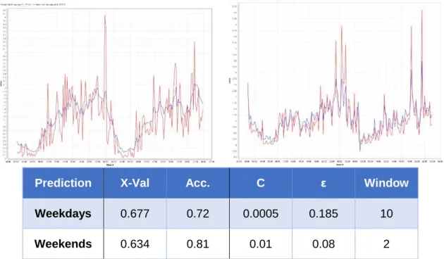
Fig. 4. 5 Regression prediction of Throughput separating weekdays (left) from weekends (right) (real values in red, predicted in blue) ... 37

Fig. 4. 6 Regression prediction of PRBs in cell 1C (left) and 8A (right) (real values in red, predicted in blue) ... 38

Fig. 4. 8 Classification accuracy and confusion matrix ... 40 Fig. 4. 9 Clustering centroid table ... 41 Fig. 4. 10 Cells clustered by load: very high (red), high (green) and medium

(yellow) ... 42 Fig. 4. 11 Comparison of real (red) and synthetic (blue) traces in cells 1C (top

left), 8A (top right) and 1A (bottom) ... 43 Fig. 4. 12 Example of Random Tree extracted from the traces ... 44 Fig. 4. 13 Cell activity in a simulation of one day, with the naïve algorithm ... 44 Fig. 4. 14 Cell activity in a simulation of one day, with the neighbour-aware

algorithm ... 45 Fig. 4. 15 Total migrated and unserved UEs in a simulated scenario with naïve

switching algorithm ... 46 Fig. 4. 16 Total migrated and unserved UEs in a simulated scenario with the

neighbour-aware algorithm ... 46 Fig. 4. 17 Power consumption during a day in a simulated scenario with a naïve

algorithm ... 48 Fig. 4. 18 Power consumpation during a day in a simulated scenario with a more

sophisticated algorithm... 48 Fig. 4. 19 Comparison of migrated UEs and power saved with different switching

strategies ... 49 Fig. A. 1 Regression prediction of DL Throughput (top) and #UEs (bottom) of 3

days in cell 1C (real in red, predicted in blue) ... 61 Fig. A. 2 Regression prediction of DL Throughput (top) and #UEs (bottom) of 3

days in cell 8A ... 62 Fig. A. 3 Regression prediction of Throughput (top) and #UEs (bottom) of 3 days

in eNodeB 3 ... 63 Fig. A. 4 Regression prediction of Throughput (top) and #UEs (bottom) using the

aggregated traffic from two eNBs (1 and 3) ... 64 Fig. A. 5 Regression prediction of Throughput separating weekdays (left) from

weekends (right) ... 65 Fig. A. 6 Regression prediction of PRBs in cell 1C (left) and 8A (right) ... 66 Fig. A. 7 Regression prediction of PRBs with granularity of 15 (top) and 30

minutes (bottom) (real values in red, predicted in blue)... 67

Fig. B. 1 Cells clustered by load: very high (red), high (green) and medium (yellow) ... 69 Fig. C. 1 Comparison of real (red) and synthetic (blue) traces in cells 1C (top left),

8A (top right) and 1A (bottom) ... 71 Fig. C. 2 Comparison of cells 40 (blue) and 58 (red) in a simulation, both based

on the traces of the real cell 3C ... 72 Fig. C. 3 Comparison of power consumption during a day in a simulation with a

naïve algorithm (top left), and neighbour aware with a threshold of 50% (top right), 70% (bottom left) and 90% (bottom right) ... 73 Fig. C. 4 Comparison of migrated (green) and unserved (red) UEs during a day

in a simulation with a naïve algorithm (top left), and neighbour aware with a threshold of 50% (top right), 70% (bottom left) and 90% (bottom right) .... 73

CHAPTER 1. INTRODUCTION

1.1.

The project

Since the first generations of cellular networks, vendors collect enormous amounts and varieties of data, which are stored in various formats, and later processed or ignored, just to be erased after short periods of time. All these data, which until some years ago were neglected, can provide useful information about how a network works, which are its strengths and weaknesses, etc. In this thesis we argue that these data can even contribute to an enhanced real-time management.

The data collected and stored by the operators belong to different categories (network, user, content, external data), are collected by different entities (network nodes, UE reports) and provide information about network traffic, resource access, QoS, cell availability, etc. The usage of these data may vary depending on the functionality we have in mind, considering both scenarios, where long-term information is required (such as network planning actions based on the records of the network over time) or real-time optimization techniques based on the latest metrics. Raw data are useless and difficult to work with, reason why there are some initial steps that have to be performed over the sets of information before starting to work with them.

The paradigm that the approach of the fifth generation networks (5G) is bringing requires the introduction of new smart mechanisms capable of analysing and correlating multiple data sources in order to extract relevant information. The scope of this project, then, consists in studying the traces of several datasets from the COSMOTE (one of the main telecommunications companies in Greece) network in Athens, build appropriate prediction models based on that data, and test some of the possible applications of such systems, for example an energy-saving mechanism consisting in dynamically switching off those cells that are unnecessary at a given time.

In order to work on that field, we used tools specialized in the field of data mining and machine learning, where the data sets provided by COSMOTE in the frame of the European project 5G-XHaul could be studied. Moreover, a simulator software tool was developed in order to test the models extracted from the data analysis, and apply them into the field of energy-saving techniques.

As the main aim of this project, we wanted to study the data extracted from a real network, see their potential, and consider a proof case of an application of such study in a realistic environment. In order to achieve these general goals, the following objectives were defined:

 Study of the literature regarding the application of Machine Learning techniques in network management.

 Familiarization with Data Analysis and Machine Learning tools, as long as with the main techniques, algorithms and working methodologies.

 Familiarization with the real network of COSMOTE in centre Athens, through several datasets.

 Generation of models based on the traces that can predict the network behaviour.

 Application of the previously mentioned models on a specific proof of concept: an energy saving technique consisting in switching off cells that are predicted to have a low load.

 Programming a simulation environment adapted to the requirements of the project and focused on the study of the effect caused by switching off cells dynamically.

With those objectives in mind, the project was planned into two main parts. The first of them consisted in the study of the data sets and use of Machine Learning techniques to obtain appropriate models in the scope of the project. The second step consists in making use of those models in one of the many possible research areas, in our case, energy efficiency in network management. To do so, a simulation environment capable of producing realistic scenarios was prepared, were different algorithms could be tested and the final results were obtained and discussed.

1.2.

5G-XHaul

This thesis is framed within the 5G-XHaul project [1], a project that has received funding from the European Union’s Horizon 2020 program [2], oriented towards research and technological development. The general objective of the project is to obtain dynamically reconfigurable optical-wireless backhaul/fronthaul with

cognitive control plane for small cells and cloud-RANs.

1.2.1. Project fundaments

The 5G-XHaul project works with the latest technologies and paradigms, such as small cells, Cloud-Radio Access Networks (C-RAN), Software Defined Networking (SDN) and Network Function Virtualization (NFV) with the aim of providing broadband connectivity in cost efficient and flexible networks, oriented towards the future fifth generation of cellular networks. Dynamic environments both in the backhaul and fronthaul architectures become a must, and 5G-XHaul

proposes a converged optical and wireless network that can connect the access and core network.

Lots of partners (from companies to research institutions or university research groups) are contributing in:

 Introducing advanced millimetre Wave and optical transceivers.

 Development of international standards through technical and economic contributions.

 Development of converged optical-wireless architectures and network management algorithms for mobile scenarios.

1.2.2. Thesis contribution

The thesis being presented here is framed in the last of the points analysed in the previous section, as we will be working with network management algorithms in cellular networks. The main contribution of this development towards the 5G-XHaul project consists in studying the traces from a real network placed in the centre of Athens and property of COSMOTE, evaluating its behaviour and generating network models that can predict several parameters of the network depending on previous values.

With the simulation environment that has been built, we have been able to test some of the proposed network management algorithms, and evaluate the results in terms of user connectivity and energy saving.

1.3.

Document structure

This document is divided into several chapters and sections in order to explain the full development of the project in a thoughtful way. First of all, an introduction to the project and the description of the main objectives have been presented. Chapter 2 presents some explanations about the theoretical basis required to understand the project, regarding both cellular networks and data analysis tools, explaining also some of the state of the art of the combination of both fields. In Chapter 3, the reader can find the main information about the tools being used for the development, as well as the data sets that were available. Chapter 4 is devoted to the main results obtained in the two big parts of the project, as explained in previous paragraphs. Finally, some conclusions and the direction of future work is presented, alongside with the bibliography that has been consulted during the project, some abbreviations and acronyms used in the report, and additional information that is collected in the annexes.

CHAPTER 2. THEORETICAL BACKGROUND

2.1.

Mobile technologies

It is important to highlight the architecture of the networks that will be studied in this thesis. As introduced in the previous section, we will be mostly working with real LTE networks, although the expansions towards the future generation of networks is worth being considered, so the basics about those standards are summarized here.

2.1.1. LTE and LTE-A

LTE (Long Term Evolution), commercially marketed as 4G1_{, is the 3GPP}

standard for high-speed wireless communications proposed in their Release 8, and based in the structure of legacy GSM, EDGE, UMTS and HSPA technologies. It is packet-oriented and designed to support high traffic loads and speeds reaching peaks of 150Mbps in the downlink and 75 in the uplink. Moreover, it was later powered up with some improvements in the subsequent Releases 9 and 10, the latter being called LTE-A (the real 4G, according to ITU-R), with an A for Advanced.

In this thesis, we are not so much interested in the functionalities and capabilities of such networks, but rather in their architecture, consisting of an access network, the E-UTRAN (Evolved-UMTS Terrestrial Radio Access Network); and the core network, the EPC (Evolved Packet Core). We will focus in the access part. The E-UTRAN is built with base stations called eNB (evolved NodeB), which are capable of managing the access network without the need of a Radio Network Controller, present in previous generations. eNBs are interconnected using an interface called X2, which allows for faster handover performance and enhanced Radio Resource Management functionalities. eNBs may also have different sectors and/or cells (it is interesting to remember that sectors are not directly bound to cells, as each cell has a different carrier frequency, and a sector may operate several frequencies and therefore several cells).

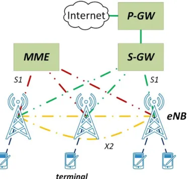
In Fig. 2. 1 we can see a simplified version of the E-UTRAN, with the S1 interfaces connecting to the EPC, consisting on the Mobility Management Entity (MME) and the connection to the outer network through the Serving and PDN Gateways (S-GW and P-(S-GW, respectively).

1 _{Despite the commercial name, it did not achieve the requirements specified by Radio} department in the ITU (International Telecommunication Union) to be part of the real fourth generation.

Fig. 2. 1 E-UTRAN and EPC in an LTE network 2.1.2. 5G

The fifth generation of networks, despite not being yet fully standardized, introduces an interesting change in the paradigm of the network architecture. The trend of 5G networks seems to be the implementation of Software Defined Radio (SDR) architectures where the intelligence, which may be running over a Software Defined Network (SDN) platform, is separated from the RF unit.

Wireless base stations will first have a baseband processing unit, called BBU (BaseBand Unit), which will be placed in some centralized equipment room, possibly with other BBUs, forming a BBU-pool. These devices will be connected to the RRH or RRU (Remote Radio Head, also known as Remote Radio Unit) via fronthaul links (including both optical fibres and wireless links). BBUs will be highly customizable and upgradable, and are in charge of most of the functionalities of the network, besides those related to the physical transmission of the signal, which are derived to the RRH.

Meanwhile, SDN (as defined by the Open Network Foundation) seems another interesting paradigm for the management of future networks. SDN provides a dynamic environment in which the network can be easily and automatically reconfigured thanks to the decoupling of the control plane (where decisions about traffic forwarding are taken care of) from the data plane (traffic forwarding). SDN integrates really well with SDR thanks to the hierarchical architecture that it introduces, as it is divided into three main layers (Applications in charge of the network management decisions, the Controller programming the network devices, and the Network devices themselves, the dumb infrastructure in charge of the forwarding plane) interconnected through totally programmable interfaces (a northbound interface that is, in general, an API (Application Programming Interface); and a southbound interface that communicates the controller with the devices, and generally is managed by the OpenFlow protocol).

As a conclusion, we can say that current and future networks have been evolving towards a combination of different techniques that may vary from fully distributed scenarios where the intelligence resides in the base stations (eNBs) and network terminations must coordinate to provide an optimal performance; to centralized intelligent devices that manage a network consisting of dumb terminations that are only in charge of the physical radio functionalities. One of the hot topics in this field consists on minimizing the power consumption in such networks, maybe using the collected data to study the behaviour of the network and improve the efficiency in their operation. There exactly is the point in which this thesis is focused.

2.2.

Machine Learning

This section is devoted to provide some understanding on what machine learning

techniques are, how can one work with that -relatively new- paradigm, and what type of results can be achieved with different problematics.

2.2.1. Concept

The field of computing in charge of studying how computers can learn on their own with the minimum human interaction has seen a great increase in popularity in the last decades. It is also true, though, that generally there are slight misunderstandings between similar concepts, and despite being used for the same purpose, each of them is specialized in a different area, and have a varying scope depending on how vast is the field they cover. In the following paragraphs, we will try to shed some light on those concepts.

2.2.1.1. Artificial Intelligence

Artificial Intelligence (AI) is a broader, older concept that aggregates all the knowledge related to how machines can have some kind of autonomous intelligence that provides them with the skills to work as a human would.

The classical understanding of AI works over the knowledge based approach, which tries to extract rules that represent some simple knowledge that can be reproduced. For example, playing chess is a task that can be based on knowledge, as a machine just needs to know the allowed movements for each piece and the objective of the game. Meanwhile, there are more complex tasks that are difficult to develop using simple rules, such as recognizing an object in an environment, as the object can be in different positions, sizes (further or closer to the camera), etc.

AI is used for general concepts such as speech recognition, planning or problem solving, although for specific tasks in which the volume of data cannot be handled or the problem is too complex to be solved with rules extracted from the current knowledge, the basic approach of AI is not enough.

2.2.1.2. Machine Learning

Machine Learning (ML) is a new approach under the umbrella of Artificial Intelligence that suggests that machines should be able to learn by themselves. Instead of providing them with repeatable knowledge, we should just give some raw data from which certain patterns can be extracted and learn from them as a human mind would.

The concept of Machine Learning was coined by one of the pioneers of AI, Arthur Samuel, in 1959, although one of the most widely used definitions is the one presented in [4] by another American computer scientist, Tom Michael Mitchell, on a book published on 1997, which says: “A computer program is said to learn from experience E with respect to some class of tasks T and performance measure P if its performance at tasks in T, as measured by P, improves with

experience E.”. In easier words, experience (i.e. input data) in a certain task is

used to learn how to work with a certain problem.

The difference between traditional AI and ML can be easily understood with the following example: it is not the same to program a code that teaches a robot how to walk, or to program one that lets the same robot learn to walk from its own experience (using, for example, statistics of forces applied on each leg, direction on which it fell, stability…).

ML is a very wide computing field that has been under study for the past years and it has reached a peak in popularity recently, with lots of companies of all type devoting resources to research in this area. There are many different approaches to ML, depending on the available data and the problem we want to solve, but that will be studied in depth in section 2.2.2.

2.2.1.3. Big Data

Enterprises of all type have insane amounts of data from which interesting knowledge can be extracted. Every transaction, customer profile or client behaviour can be gathered with others of the same type to extract information that can be useful for the company itself or for others. For instance, the click stream on a web page, the feeds provided by a certain topic in Twitter or the aggregated power consumption in the power grid of each neighbourhood in a city, are reliable sources of data that, studied and processed in the correct way, can result in the transformation of unstructured and scattered data into a summarized specific piece of knowledge.

The Computing Community Consortium (CCC) is an association whose objective is to offer guidelines for the computing research community, articulate different perspectives and interact with policymakers, governments, the industry and the public. It revived the concept of Big Data (concept already coined in 1997 by astronomers Cox and Ellsworth) on 2012 with a White Paper [5] in which the main things about what Big Data is supposed to be are summarized and offers a pipeline about how this process should work (Fig. 2. 2).

Fig. 2. 2 Reproduction of the CCC Big Data Pipeline presented in [5]

So, as seen in the presented pipeline, it is a general structure of how to obtain information from several inputs, based on the following steps:

 Acquisition and Recording: obtain the data from a reliable source and apply the appropriate filters so as to delete that part of the data that is not interesting (take into account that we may be talking of large amounts of data, in the order of TeraBytes or PetaBytes) without discarding useful information. It also comprises the process of generating the appropriate metadata to describe the type of data being recorded and how it was recorded and measured.

 Extraction and Cleaning: we need to extract structured information from the raw data collected and recorded, and clean it so that no outliers (missrecorded or out-of-pattern information that will worsen the obtained model) or errors are passed to the following steps in the chain.

 Data Integration, Aggregation and Representation: integration consists on providing automatized tools that are capable of producing computer-understandable data from what we already have. Then, data must be

aggregated by similarity, putting together everything that can or must be

processed in the same way. And finally, depending on the type of data being processed, it is also important to find a proper representation

scheme in which aggregated information can be easily visualized.

 Data Analysis and Modelling: the noisiness and heterogeneity properties of Big Data makes it necessary to find adequate querying and mining techniques to extract the information we really need from the vast amounts of data that are available. Performing some analysis over the data, different models can be obtained, which lead us to the last step.

 Interpretation: at the last step of the process there is generally a decision-maker that is in charge of interpreting the results of the whole process and offer a final solution that can be easily understood by the user.

Nevertheless, the Big Data pipeline is constrained by the main challenges also presented in the diagram, which are: heterogeneity (Big Data is generally highly heterogeneous and incomplete, so it generally must be cleaned, corrected and completed), scale (CPU cores parallelism and cloud computing are two new

paradigms about which Big Data engineers did not have to worry in the past), timeliness (sometimes we need immediate results from the analysis process), privacy (both for the public and for companies, it is a big concern how their data is being treated) and human collaboration (instead of building completely autonomous systems, it might be interesting to have a human in the loop, who might be able to solve some simple problems that are difficult to devise by a machine).

Also, as defined by Oracle, a leading company in the software industry, in [6] and [7], Big Data is defined by the four Vs:

 Volume: companies and institutions own large amounts of data, however, it is generally unstructured and its properties are unknown. Depending on the type of data being treated (text files, graphs, images…) and the size of the Data Base (DB), the proportions of the data may vary in a big scale, from some gigabytes of text files to hundreds of petabytes in images.

 Velocity: depending on the application given to the collected data, the operation velocity and technique may vary. From data from several months written to disk and analysed once the experimenting period is ended, to real-time applications where it may be streamed directly into memory so as to process it on the fly.

 Variety: data has to be different enough so as to provide information. Entropy (as defined by Shannon, it is the amount of data contained in a message) is found in unstructured data that shares enough features so as to be considered of the same type, but is sufficiently uncorrelated so as not to have overlapping knowledge.

 Value: nearly all data has intrinsic information that is, in most of the cases, yet to be discovered. There are many examples in which data was already being collected for other purposes, but was not exploded to obtain additional information. This value can be extracted using different Data Mining techniques. This term is generally comprised under the Big Data one, although being completely strict on their definitions, Big Data refers to the sources of information themselves, while Data Mining refers to the processes applied to that unstructured data so as to obtain knowledge. Big Data and Data Mining have suffered a huge increase in popularity in recent years, because with relatively small effort (in most of the cases the data was already collected, so we “just” have to study it) really good results can be achieved. Moreover, the cost of storage and computing resources has drastically dropped in the last decade, so it is becoming easier and easier to store enormous databases and process them using efficient techniques. There are also some companies that are beginning to specialize in offering services related to this field, such as Amazon with its elastic computing platform (EC2 [8]), Microsoft with Azure [9], OpenStack [10], etc.

2.2.2. Algorithmic

Machine Learning techniques are based in different types of algorithms, and the decision to use one or another depends, basically, on the type of data we have and the type of output we want to obtain. The objective of this subsection is to

present all the algorithms that may be used at some point during the development of the project, as well as some other useful tools. There are many other algorithms and techniques that cannot be included in this text due to extension restrictions, so this thesis report is limited to those techniques that have been somehow considered for the development of the project.

2.2.2.1. Unsupervised algorithms

Unsupervised learning consists in obtaining some function that can describe the structure of some unlabelled data, i.e. we just offer some raw data to a given machine (which, of course, should have previously gone through the first steps of the Pipeline in Fig. 2. 2) which will provide us with a function to group the data into different sets with certain similarities.

Probably, the most popular unsupervised technique is Clustering. Clustering uses ML to group (or technically speaking cluster) data into several entities considering the similarity of the features that data has. Generally speaking, clustering is difficult to evaluate, as there is no labelled data set with which to compare results. Each data sample is described by a vector of N features x that can be used to represent it in an N-dimensional space. The distance metric used to determine the closeness between points is really important, as it can drastically change the results. In most of the cases, Euclidean distance (the distance in a straight line between any two points in an Euclidean space) is used, although other more complex techniques can also be applied.

Some of the most common clustering algorithms are:

 K-Means: the algorithm groups the data samples into k clusters. To start,

each cluster selects a random centroid and data entities are associated to a cluster according to the shortest distance to each of the centroids. Then, the centroid is moved to the central point (mean value) of the cluster, and the new distances between entities and centroids are computed. The process keeps iterating until each of the data entities is closer to its centroid than to any other, resulting on something similar to this:

Fig. 2. 3 K-Means clustering result on a 2-dimensional space

 Hierarchical Clustering: each data entity represents its own cluster, which

is in the following iteration merged with the closest cluster. With this technique, we can cluster data into k clusters without previously knowing this value k, as the algorithm will try to find the optimal solution. We have an example in Fig. 2. 4.

Fig. 2. 4 Hierarchical Clustering example

2.2.2.2. Supervised algorithms

Supervised learning techniques are those that include some labelled feature on each data entity. Data sets used with this ML technique include a set of features, which are the variables considered on each sample, and generally a single labelled feature, which can be a figure (generally in regression) or a text (generally in classification) and identifies the most important variable of the entry, the one that identifies it.

The general idea is to split the data set into some training and test set (the first one is used for training the model that is generated, while the second one is used to test that same model and check the results), using one of the multiple available options: naïve (just splitting the dataset by some percentage), cross-validation (split the dataset into K = M + N equally-sized folds, using M for the training, N

for the test and then cycling over them until we can get the mean and standard deviation of each of the folds), nested cross-validation (an even more complex yet effective cross-validation technique), etc.

Then, we can compare the obtained results with the real values. To do that, we input the test set into the model deleting the label column, and then we just compare the suggested label with the real one.

Depending on the problem to be faced, we can use different solving paradigms:

 Regression: use data with known values to predict the labels of other similar data entities. Regression identifies real numeric values using a function y = f(x) that labels new data entities y (i.e. predict the behaviour of a given feature for a given new data entity) according to the model obtained from all the previously known feature vectors x. Some specific regression algorithms are:

 Simple Linear Regression: use a simple linear function such as (X)

to predict the value of f(xi).

𝑓(𝑥_𝑖) = 𝑏₀ + 𝑏₁𝑥_𝑖

 Ridge Regression: use a more complex function to predict a value

f(xi), also considering samples from different time instants t in xi,t. 𝑓(𝑥_𝑖) = 𝑏₀+ 𝑏₁𝑥_𝑖,1+ 𝑏₂𝑥_𝑖,2+ 𝑏₃𝑥_𝑖,3

(X)

 Support Vector Machine (SVM): it is a variation of ridge regression in which the loss function (the function that defines the error committed in the assignment of the label as compared to the real value) is modified. SVM is one of the most popular algorithms, and can be also used as a classification technique.

 Classification: classification techniques assign a label (from the N ones available) to an unlabelled data entity. All entities from the test set end up with a label that can be later compared to the real ones and measure some typical statistics:

Table 2. 1 Confusion Matrix

Predicted Positive Predicted Negative Actual Positive True Positive (TP) False Negative (FN) Actual Negative False Positive (FP) True Negative (TN)

 Accuracy: calculated as in (X), provides the percentage of accurate

predictions.

𝛼 = 𝑇𝑃 + 𝑇𝑁 𝑇𝑃 + 𝑇𝑁 + 𝐹𝑃 + 𝐹𝑁

 Precision: calculated as in (X), provides the percentage of guessed

values for each class.

𝜌 = 𝑇𝑃 𝑇𝑃 + 𝐹𝑃

 Recall: calculated as in (X), measures the fraction of guessed

instances over the total instances. 𝑟 = 𝑇𝑃

𝑇𝑃 + 𝐹𝑁

 F1 score: calculated as in (X), is a combination of both precision and recall.

𝐹1 = 𝜌 · 𝑟 𝜌 + 𝑟

 Some popular classification algorithms are:

 SVM: the same as in regression, but now providing a given class

as an output.

 Decision Tree: a sequence of branches is defined; at each

intersection, a given function is calculated and, depending on the result, one or other branch is followed. In Fig. 2. 5 , an example tree can be seen, which can be used to classify people depending on several features such as their age range, education, activities, etc. Trees have different properties, although one of the most important may be the total depth of the tree, i.e. the amount of levels of branches it has plus the root. In this example, the tree in Fig. 2. 5 has a depth of 4. This parameter is important because deeper trees may be more accurate, but having really deep trees may lead to

(X)

(X)

(X)

overfitting to the training set, which is an undesired side-effect; on the other hand, fewer levels is more simple to compute and execute, but may be too generic. Imbalanced Data Sets (DS), which are those where a class highly predominates over the rest or has many less samples than the others, can be solved by weighting the samples to balance the algorithm.

Fig. 2. 5 Decision Tree example

 Random Forest: a random forest works as a set of N differenttrees

that are run with the same input data and that may produce equal or different results. The output of all the trees is then combined (using different techniques, such as majority voting, average of the results, etc.) and a single solution is provided. The random part about these forests is that all trees are different thanks to using different random seeds for their generation, and the diversity of the trees can be configured by tuning some parameters.

 One vs. all: multi-class technique that extends any binary

classification algorithm to support more than two classes at the same time. It works by performing the function y = f(x) over all the possible classes and comparing the y results to see which is the class it has more confidence in.

2.2.2.3. Reinforcement learning – Neural Networks

Reinforcement learning is the last of the main ML paradigms considered for the development of this project. This set of techniques consists in the fact that the system interacts with the environment with a feedback loop, so that each output has an effect over the current model that produced it.

Neural Networks, are based on the methodology of reinforcement learning, by imitating simplified biological learning models such as neurons. Neurons are very simple computational units that produce an output according to some stimulus. The interconnection of an extremely large amount of neurons with high connectivity, plus the capacity of working in parallel, can produce amazing results in the field of ML.

Neurons, as represented in Fig. 2. 6, are computing entities with several inputs

xN and some links wN that connect and weight each input. It also has a bias value

Fig. 2. 6 Example of a Neuron in ML terminology

Neurons can train themselves using the real and desired output depending on different approaches that have been relieving each other all along their history. For instance, the first approach, the Hebb Rule (1949) [11], reinforced those outputs that were correctly predicted; the Perceptron (1950) [12] is just the opposite, using Negative Learning (reinforce the errors); and AdaLine [13] reinforces both cases with an error e that is measured as the difference between the desired and real outputs.

Up to now, however, we have only seen how a lonely neuron works. Neurons can be combined to form a neural network that can produce way better results. We can even add hidden layers to form deep neural networks (as in Fig. 2. 7) that can solve any kind of problem, although their understanding and design is out of the scope of this project.

Fig. 2. 7 Example of Neural Network with 1 Hidden Layer

2.3.

State of the Art

The objective of this section is to present the state of the art related to the main topics covered in this project. First of all, we give details of the latest investigations about the application of ML to network management, and then we review the literature on power management in mobile networks.

2.3.1. Machine Learning techniques for network management

2.3.1.1. Traffic profiling in radio networks with Machine Learning

As already commented and presented in [11], BigData technologies will play a really important role in the deployment of the future 5G networks, as they are able to transform vast amounts of data into something valuable that can be used, for example, to improve the performance of the network. This paper intends to develop intelligent systems capable of studying the environment, identifying patterns and working with an AI-oriented network control plane. It focuses on using classification to identify patterns in the cells deployed in the network and classify them in a set of known classes. Two main use cases are presented, although only the first one is relevant to our project:

 Use case 1: energy saving by means of switching off cells that carry very little traffic at given times of the day. Cells are classified into two classes (candidates to be switched off or not). The input vector to the machine learning algorithms will have 21 components (7 days of the week, 3 time intervals, with the average normalized traffic of the cell), and each of the 4 classification techniques used is tuned manually so as to achieve the optimal solutions. The classifiers will work with 419 cells that offer measures every 15 minutes, and the traffic is measured as the average number of users in the cell with an active data session. Only sets of 10-200 cells are used for the training, and the best results are provided by SVM and Neural Networks, as measured by the percentage of total coincidences between the classification tool and the category assigned by the expert validation. Section 5.2 in [11] presents the optimum parameter values for each of the classifiers.

 Use case 2: there are several new considerations of LTE regarding the spectrum usage, such as using unlicensed bands (LTE-U) or sharing the spectrum with a primary user (within certain limits). In this case, cells are classified into two classes (candidate cell to boost capacity through additional unlicensed spectrum or cell that does not need the boost). Now, traffic is not normalized (the absolute value is also important), and only 16 components (daily basis, 1 component per hour from 6am to 10pm) are used, with the same classification tools as in the previous use case.

There is another project in [18] whose objective is to estimate the load of a given group of base stations just from the monitoring of the load of a subset of those. The accuracy on the predictor will vary on the base stations chosen for the monitoring (amount and type). To do so, OLS (Ordinary Least Squares) is considered, a linear regression technique that, despite being popular, has poor accuracy, reason why an alternative is presented: Lasso (Least Absolute Shrinkage and Selection Operator). The data used for the prediction is formed by

TCP/UDP flows from 400 base stations along 5 days (weekdays). As the variation in traffic patterns all along the day is really high, they divide the data and create models for individual periods of 4h, thus getting 6 separate models for each day. In conclusion, good results are obtained, both with classification techniques (SVM and Neural Networks) and regression (improved OLS). They are all supervised algorithms, which implies that the training set has to be assessed by an expert, who would manually identify the example cells as one or other class.

2.3.1.2. Using clustering to group entities with similar characteristics

Grouping cells in a network by similar features is another interesting technique that is being exploited in the literature. In fact, most of the sources consulted perform some type of unsupervised clustering algorithm to subdivide the traffic profiling problem into smaller parts.

In [15] two different clustering methods are used, K-means and Gaussian Mixture Models (GMM). K-means is a simple method that works well for low dimensional data (while it gets slow for large data sets), which may be able to find local (but not global) optima and has problems with outliers and noise. In this case, they cluster the users, not the cell types, and the simulation that is run is based on the following items:

 Model based on an American city with a city centre and high population density, surrounded by a highway and a suburban area with low population density.

 11 base stations, 33 cells, 600 active users.

 60 minutes with 100ms time step.

 Use of several type of users (indoor, low mobility, medium mobility, high mobility).

 Users downloading 1MB files.

The features are similar to the one in the real COSMOTE data sets we have available for the project, and with the provided results, we can conclude that user classification may not be a promising solution for the problem being boarded. Tree classification models are able to perform automatic variable selection, being this an advantage if we don’t know which features (if any) are more important than others when performing the classification. However, Trees tend to result in a quite low accuracy, reason why Random Forest are used instead. Random Forest works with several decision trees that are aggregated together so as to improve accuracy, being also more robust to overfitting, as each tree will work with a different part of the original training data, and there’s always a factor of randomness involved.

Using the clusters identified in the clustering process, they train and test the classification Random Forest algorithm. They also study the importance (Gini index) of each of the 5 variables that are being taken into account (time to handover, user throughput, CQI, number of active users and cell throughput), and how the behaviour of the classifier would change if one of those statistics went missing. The results obtained in [15] prove that training on a 1/60 of a time frame still offers accurate classification results for the rest of the time frame.

There is another really interesting research in [16] that introduces new concepts not seen in similar papers. It investigates the prediction of hourly traffic volumes based on historic data, with the goal of provisioning an energy efficient system. In order to remove redundant information, obtaining only the stable information, wavelet decomposition is used, as well as other techniques:

 K-means clustering method to automatically classify data into K groups.

 Wavelet transform, a data processing tool that works at different frequency scales or resolutions. This procedure helps dividing data into more stable and tractable sets, which can then be processed individually, obtaining a higher overall prediction accuracy. Moreover, this method ensures orthogonality, which will help with the predictions.

Fig. 2. 8 Forecasting framework proposed in [16]

 As the prediction algorithm, an Elman Neural Network is used. It is a powerful tool for predicting time sequences, based on an input layer, a hidden layer and an output layer, with a fourth context layer that feeds back the state of the outputs of the hidden layer without weighting. The problem presented in this project is highly nonlinear, reason why ENN was chosen as the method for the prediction, as its ability to store internal values helps in the approximation of nonlinear dynamics.

Some results regarding clustering and framework (Fig. 2. 8) accuracy are presented in Fig. 2. 9:

Fig. 2. 9 Clustering results (left) and traffic load prediction relative error (right) achieved in [16] Finally, in [17] a project is presented whose main aim is to identify clusters of cells with similar 24-hour traffic profiles. To do so, besides removing some outlier cells (158 from the original 2175 cells), the data was cleaned so as to take only the relevant information (hours 8 to 23, only weekdays, as the rest didn’t follow any pattern that could be modelled). The clustering process helped them with the classification of cells into 6 different groups, which lead to an improved estimation of the required capacity between a 25 and an 80% (as seen in Fig. 2. 10).

Fig. 2. 10 Real traffic (left) and predicted by the cluster-based model (right)

2.3.2. Power management in mobile networks

As for the project developed during this thesis, it is also interesting to take into account the literature regarding power management in radio networks, as one of the applications is to provide energy efficiency to an access network scenario. [19] discusses the performance of a scenario where the cells with idle capacity requirements are turned to sleep mode. Based on other references, this paper evaluates the potential performance of an energy-saving scheme where underutilized cells are put to sleep, as LTE eNBs have a significant power saving when working on idle mode, as can be seen in Fig. 2. 11:

Fig. 2. 11 Assumed model for the eNB power consumption over time [19]

Pin,A represents the power consumption in active state, Pin,I in idle state, and 𝛿 ·

Pin,I is the result of using fast cell DTX (Discontinuous Transmission) [20], where

0 < 𝛿 < 1 and in the paper is generally assumed to be 𝛿 = 0.1.

Meanwhile, [19] studies different network deployments and cell DTX to reduce power consumption, with the results summarized in Fig. 2. 12. The left graph shows which network distribution achieves lower consumption, while the right one represents the consumption over a day, and the heavy energy saving at night, during the low-traffic hours, where a reduction of up to 49% is achieved, given that during that period of time, cells are in idle mode for 98% of the time. This reinforces the hypothesis presented on this thesis about considering valley hours as the reference for cell type clustering and switch-off algorithms.

Fig. 2. 12 Normalized daily energy consumption for the different network densification alternatives (left) and total power consumption of the sleep mode deployment as a function of

time without fast cell DTX (solid curves) and with fast cell DTX (dashed curves) (right)

Finally, [21] presents their own joint access-backhaul SDN platform for efficient management of a radio network. The research devoted to energy efficiency uses a similar technique to what is originally thought for this project, i.e. turning on and off access nodes dynamically to achieve energy saving, and they also highlight the importance and consequences of eliminating access nodes from the network. To do so, they run an algorithm that, besides identifying the potential candidates to be switched off, it adds three Quality of Experience (QoE) constraints:

 Network coverage: failure probability that a user loses connectivity.

 Admission control: blocking probability for flows with dedicated bandwidth.

 Delay for best-effort flows: flow delay exceeding a given threshold.

So this paper raises the problematics that appear when switching off some access nodes of the network, which is something that has to be considered.

CHAPTER 3. TECHNOLOGIES AND ALGORITHMIC

This chapter is devoted to the description of the main software, technologies and data sources used for the development of the project. Starting with the 5G-XHaul project and the provided data sets, we later go into using RapidMiner for Machine Learning purposes, and finally a brief explanation of the main functionalities of the simulator designed for the thesis.

3.1.

5G-XHaul

As explained in section 1.2, this thesis is framed under the 5G-XHaul project, and therefore we have had access to real data from UMTS and LTE networks from COSMOTE2_{, a Greek mobile telephony company. This section is devoted to}

explaining the characteristics of the networks from which we had accessible data, and also describing the datasets we were provided with.

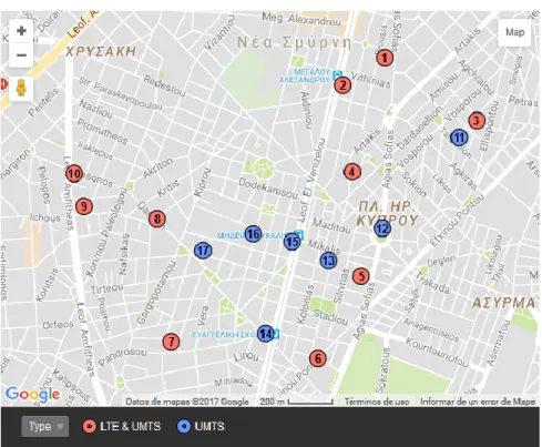
3.1.1. Real scenario

The datasets provided by COSMOTE include 17 BTS located in centre Athens, 10 of which have both LTE and UMTS cells, while the 7 remaining only support UMTS. The approximate location of the base stations (BTS) from which we have data is depicted in Fig. 3. 13_.

Fig. 3. 1 COSMOTE network BTS location

2_{https://www.cosmote.gr/hub/} 3_{https://es.batchgeo.com/}

Athens is a heterogeneously dense city which, in an area of around 750 km2

(including dense urban, urban and suburban areas) has a deployment of over 600 LTE eNodeBs. Note that, on the same area, second generation, UMTS and HSPA+ sites are also deployed, but our interest is focused on LTE. With such figures, the average density in the city is about 0.8 eNBs/km2_{, although there are}

some additional considerations in scenarios with a maximized density:

 In really dense areas, such as the city centre, there are more than 30 eNBs with over 70 sectors in 1 km2_{, which is makes a density of 10 eNBs / km}2_.

 In suburban areas, the density may be around 2.5 eNBs/km2_.

In those deployments, LTE eNodeBs are configured to offer a coverage range that moves between 100m and 600m, corresponding to different type of cell deployments depending on the geographical area being covered. The power consumption of those eNodeBs are unknown figures, so we will assume the values given in [19] (Table 3. 1) as a coarse approximation. PeNB,max is the maximum eNodeB output power, while Pin,A and Pin,I correspond to the consumed power per cell in active or idle mode, as represented in Fig. 2. 11. Table 3. 1 eNodeB power consumption model from [19]

eNodeB Type PeNB,max [W] Pin,A [W] Pin,I [W]

Macro RRH 40 336.3 238.4

Micro 1 152.4 129.3

Femto 0.1 16.6 14.4

The sites available in the COSMOTE network have from 1 to 3 cells and, in general, they have a bandwidth of either 20 (in most of the cases) or 10 MHz.

3.1.2. Data sets

For the development of this project, we were provided with 2 packs of data sets. They are two independent data sets covering 15 days each; the first of them is on the last trimester of 2015. In both cases, we have 15 days of data statistics collected every 15 (for the LTE cells) or 60 minutes (for the UMTS cells), including two weekends, where the traffic profiling may be different.

As for the statistics collected during each quarter hour from the LTE cells, they are written on a spreadsheet with different pages, one for each BTS, and there can be found many different metrics. The ones that have been studied in deeper detail for the development of the project are those that are underlined. The rest were considered finally not as relevant, and there are some more metrics that do not cover any important feature considering the development.

 Time: time variable including the date and time of the sample.

 Cell Name: text variable including the ID of the cell with the format XYLTE, where X is the BTS ID and Y the cell ID inside the BTS.

 Mean Cell Throughput (Mbps): average LTE UL/DL throughput in Mbps.

 Max Cell Throughput (Mbps): maximum LTE UL/DL throughput in Mbps.

 Average # UEs: average number of UEs each TTI (Transmission Time Interval).

 Max #UEs: maximum number of simultaneous UEs in a TTI.

 Total UEs in eNB: total UEs in eNB during the whole hour.

 Average PRB Usage per TTI (%): UL/DL average Physical Resource Blocks usage (i.e. PRBs Used / PRBs Available) per TTI.

 Intra eNB Latency: Intra eNB latency.

 Average CQI: average Channel Quality Indicator (CQI).

 CQI Distribution per Level (00-15) (%): CQI distribution per level for each of the 16 CQI values as percentage of total samples.

 MCS Distribution per Order (%): % distribution of Modulation and Code Scheme (MCS) usage (Low (MCS0-9), Medium (MCS 10-19), High (MCS20-28)).

 MCS Distribution per Scheme (MCS0-MCS28) (%): MCS distribution per Scheme for each of the 29 values as percentage of total samples.

 Average PUCCH SINR: average PUCCH SINR.

 Average PUSCH SINR: average PUSCH SINR.

3.2.

RapidMiner

This section is devoted to explaining the tool with which the first half of the project has been mostly developed. In the first steps of the thesis, there has been a big involvement with data analysis and identification of predictive models for the COSMOTE traces.

The tool chosen for the development of this progress is RapidMiner [22], and the aim of this part of the chapter is to familiarize the reader with RapidMiner and to give a basic how-to so as to understand the incoming sections that go deeper into the understanding of this software.

3.2.1. What is RapidMiner?

RapidMiner is an integrated data analytics platform that offers a unified environment for machine learning-related projects. The platform has three main products: Studio (the one used in the project and that will be commented in-depth later), Server (a platform to deploy online projects from Studio) and Radoop (a Hadoop [23] implementation for RapidMiner).

RapidMiner Studio is the tool that has been used for the project and, as defined in the official website, it is a “powerful visual workflow designer for rapidly building predictive analytic workflows. This all-in-one tool features hundreds of data preparation and machine learning algorithms to support all your data science projects”. So, in short, it offers a graphic interface in which, by means of boxes that perform different functions, we can program data analytics projects.

RapidMiner Studio offers a free version with a limitation of 10.000 rows of input data (which in general, for a relatively small project, might be enough, although we have worked with some larger datasets in some particular experiments). It also has an Educational program with unlimited dataset size, and further licenses with improved performance capabilities.

3.2.2. How to

RapidMiner offers an easy-to-use difficult-to-master platform that, by means of being visual, is accessible for anyone without even basic programming skills. It also offers a huge variety of extensions (either created by the community or by the developer team) that can be purchased, and for this project, the Series Extension pack [23] has been key.

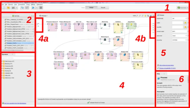
In the screenshot Fig. 3. 2, we can see the RapidMiner Studio workplace, with some information about the different parts of the software: 1 are the toolboxes, 2

shows the datasets and the projects that have been imported to RapidMiner, 3

includes all the modules available and a search box to find them easily, 4 is the main process window where the project is developed (4a are the inputs of the project and 4b the outputs that will show once the program is executed), 5 are the options available for each of the modules (boxes) in the project, and 6 is a help window that explains the functionalities and options of each of the modules.

Fig. 3. 2 Screenshot of the RapidMiner Studio workplace

RapidMiner offers a really wide variety of operators that can be further complemented with free and paying extensions. These are some of the most important sets of modules:

 Data access: import data from different sources (files, databases, cloud, Twitter feed...).

1

2

3

5

6

4

4a

4b

 Blending: modify the data set by changing some values or filtering attributes.

 Cleansing: adapt the dataset by performing multiple functions such as normalization, replacing missing values, getting rid of duplicates or outliers, etc.

 Modelling: it offers up to 129 different algorithms for regression, segmentation, weight calculation, optimization of parameters…

 Scoring and validation: finding the final performance results, as well as the confidence on them and additional cross-validation modules.

 Other: execute external scripts or macros, log information, generate random data, divide processes…

 Series Extension: the additional Series Extension is needed to work with time series, which is what is being done in the project, predict a future sample from the preceding ones. This extension offers the Windowing

module, which basically stacks N samples in a single row so that all the parameters from those N samples can be considered part of a single prediction. An example is shown in Fig. 3. 3. The Series Extension also offers specific metrics designed for time series.

Sample A B 0 10.3 26.2 1 15.0 35.3 2 9.6 20.4 4 … …

Fig. 3. 3 Dataset modification performed by the Windowing operator with window_size = 3

Just to end with this section, below (Fig. 3. 4) the reader can find a brief explanation of how a simple prediction project works.

Fig. 3. 4 RapidMiner example project: predicting mean cell throughput

The figure shows an easy example of how to predict the parameter Mean Cell

Throughput (cf. section 3.1.2) on a given cell. It works as follows: after the input

file is chosen (in our case the dataset for eNB1) 1 is in charge of pre-processing

Sample A - 2 B - 2 A - 1 B - 1 A - 0 B - 0 0 9.6 20.4 15.0 35.3 10.3 26.2 1 … … … …

1

2

4

3

5

the data by cleaning it and filtering only the cell we are interested in (in this example, Cell 1C); 2 divides the training and test set by date, i.e. the first 12 days are used for training and the last 3 days are the test set; 3 is in charge of creating the regression model that, by using an SVM algorithm, will predict the next sample based on the previous ones; 4 generates the appropriate test set from the data; and finally 5 cleans the output data so that it can be represented in an understandable way, while also providing some additional metrics about the accuracy of the model.

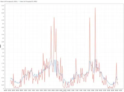
The prediction output of the project above can be seen in Fig. 3. 5, and it also outputs a performance accuracy of 0.708.

Fig. 3. 5 Output prediction of Fig. 3. 4; in red the real values, in blue the predicted ones

3.3.

Working on realistic scenarios: simulation

Once the first part of the project regarding data analysis and traffic profiles modelling was ready, the project required some additional work to test everything that was learned during the previous stages. In this section, an overview of the simulation environment used for the last part of the project is presented.

3.3.1 Tools and environment

With the objective of evaluating different management strategies in a cellular network, the idea of building a simulator capable of generating realistic scenarios from the real traces in the data sets came up. It should fulfil the following requirements: it had to be realistic and based on the COSMOTE traces, it had to be fully customizable and upgradable according to the new ideas and project perspectives that could appear, it must collect statistics from the randomly generated scenarios, and it could include some graphical resources to back the results with an easier interface.