Avner May
Submitted in partial fulfillment of the requirements for the degree
of Doctor of Philosophy
in the Graduate School of Arts and Sciences
COLUMBIA UNIVERSITY
Avner May All Rights Reserved
Kernel Approximation Methods for Speech Recognition
Avner May
Over the past five years or so, deep learning methods have dramatically improved the state of the art performance in a variety of domains, including speech recognition, computer vision, and natural language processing. Importantly, however, they suffer from a number of drawbacks:
1. Training these models is a non-convex optimization problem, and thus it is difficult to guar-antee that a trained model minimizes the desired loss function.
2. These models are difficult to interpret. In particular, it is difficult to explain, for a given model, why the computations it performs make accurate predictions.
In contrast, kernel methods are straightforward to interpret, and training them is a convex op-timization problem. Unfortunately, solving these opop-timization problems exactlyis typically pro-hibitively expensive, though one can use approximationmethods to circumvent this problem. In this thesis, we explore to what extent kernel approximation methods can compete with deep learn-ing, in the context of large-scale prediction tasks. Our contributions are as follows:
1. We perform the most extensive set of experiments to date using kernel approximation methods in the context of large-scale speech recognition tasks, and compare performance with deep neural networks.
2. We propose a feature selection algorithm which significantly improves the performance of the kernel models, making their performance competitive with fully-connected feedforward neural networks.
3. We perform an in-depth comparison between two leading kernel approximation strategies — random Fourier features [Rahimi and Recht, 2007] and the Nystr¨om method [Williams and
kernel, it performs worse than random Fourier features when used for learning.
We believe this work opens the door for future research to continue to push the boundary of what is possible with kernel methods. This research direction will also shed light on the question of when, if ever, deep models are needed for attaining strong performance.
List of Figures iv
List of Tables vii
1 Introduction 1 2 Preliminaries 8 2.1 Notation . . . 8 2.2 Kernel methods . . . 9 2.2.1 Primal formulation . . . 10 2.2.2 Dual formulation . . . 12 2.3 Kernel approximation . . . 13
2.3.1 Random Fourier features (RFF) . . . 14
2.3.2 Nystr¨om method . . . 16
2.4 Reproducing kernel Hilbert spaces (RKHS) . . . 19
2.4.1 Representer Theorem . . . 22
2.5 Neural networks . . . 25
2.5.1 Backpropagation . . . 26
2.5.2 Other architectures . . . 29
2.6 Automatic speech recognition (ASR) . . . 32
2.6.1 Acoustic model training . . . 34
2.6.2 Using neural networks for acoustic modeling . . . 35
3 Related work 37
4.1 Methods . . . 43
4.1.1 Using kernel approximation methods for acoustic modeling . . . 43
4.1.2 Linear bottlenecks . . . 43
4.1.3 Entropy regularized perplexity (ERP) . . . 44
4.2 Tasks, datasets, and evaluation metrics . . . 46
4.3 Details of acoustic model training . . . 48
4.4 Results . . . 50
4.5 Other Possible Improvements to DNNs and Kernels . . . 53
4.6 Conclusion . . . 55
5 Compact kernel models via random feature selection 56 5.1 Random feature selection . . . 56
5.2 A sparse Gaussian kernel . . . 58
5.3 Results . . . 59
5.4 Analysis: Effects of random feature selection . . . 64
5.5 Conclusion . . . 66
6 Nystr¨om method vs. random Fourier features 67 6.1 Review of Nystr¨om method properties . . . 68
6.2 Experiments . . . 69
6.2.1 Task and dataset details . . . 69
6.2.2 Train details . . . 70
6.2.3 Results . . . 71
6.3 Nystr¨om method error analysis . . . 79
6.4 Conclusion . . . 82
7 Conclusion 83 7.1 Future work . . . 84
Bibliography 86
A Definitions 104
B Derivation for random Fourier features 106
C Detailed results 108
C.1 Results from Section 4 . . . 108
C.2 Results from Section 5 . . . 111
D Nystr¨om Appendix 114 D.1 Datasets . . . 114
D.2 Hyperparameter Choices . . . 115
D.3 Results . . . 115
D.4 Background for Proofs . . . 122
D.4.1 Definitions of a couple infinite dimensional Hilbert Spaces . . . 122
D.4.2 Review of Reproducing Kernel Hilbert Space Definitions . . . 122
D.5 Proofs: Nystr¨om Background Section . . . 123
D.6 Proofs: Nystr¨om Error Analysis . . . 125
D.6.1 Theorem 4 . . . 125
D.6.2 Theorem 5 . . . 128
D.6.3 Theorem 6 . . . 130
D.6.4 Theorem 7 . . . 130
D.7 Other ways of understanding the Nystr¨om method . . . 132
D.7.1 Nystr¨om method as a projection onto a subspace . . . 132
D.7.2 Nystr¨om method as a solution to an optimization problem . . . 132
D.7.3 Nystr¨om method as a preconditioner . . . 133
D.7.4 Nystr¨om method as eigenfunction approximator . . . 134
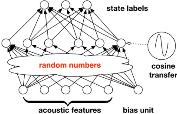
1.1 Impact of deep learning methods on state of the art performance in speech recogni-tion and computer vision. . . 4 4.1 Kernel-acoustic model seen as a shallow neural network . . . 44 4.2 Performance of kernel acoustic models on BN50 dataset, as a function of the number
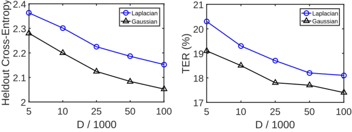
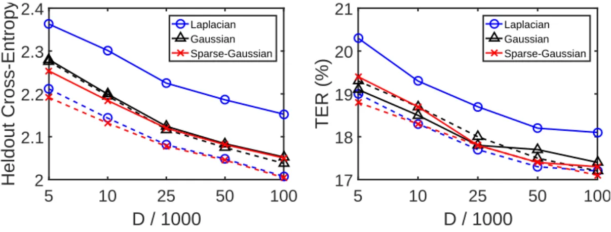
of random featuresDused. Results are reported in terms of heldout cross-entropy as well as development set TER. The color and shape of the markers indicate the kernel used. . . 54 5.1 Performance of kernel acoustic models on BN50 dataset, as a function of the number
of random featuresDused. Results are reported in terms of heldout cross-entropy as well as development set TER. Dashed lines signify that feature selection was performed, while solid lines mean it was not. The color and shape of the markers indicate the kernel used. . . 65 5.2 Fraction of thestfeatures selected in iterationtthat are in the final model (survival
rate) for Cantonese dataset. . . 66 5.3 The relative weight of each input feature in the random matrix Θ, for Cantonese
dataset,D= 50,000. . . 66
in terms of the total numbers of features (top) and the total memory requirement (bottom) in the respective models. Error is measured as mean squared error on the heldout set. For Nystr¨om experiments withD≤2500, and RFF experiments with D ≤ 20000, we run the experiments 10 times, and report the median, with error bars indicating the minimum and maximum. Note that due to small variance, error bars are often not clearly visible. . . 73 6.2 Spectrum of kernel matrices generated fromN = 20krandom training points. . . . 73 6.3 Heldout classification or regression performance for the Nystr¨om method vs.
ran-dom Fourier features, in terms of the total numbers of features (left), total memory requirement (middle), and kernel approximation error (right) of the corresponding models. For Nystr¨om experiments with D ≤ 2500, and RFF experiments with D≤20000, we run the experiments 10 times, and report the median performance, with error bars indicating the minimum and maximum. Note that due to small vari-ance, error bars are often not clearly visible. . . 74 6.4 Histograms of kernel approximation errors for Nystr¨om features random Fourier
features. The different histograms correspond to a partition of thek(x, y)−z(x)Tz(y)
values based on the values ofk(x, y). Note that the Nystr¨om method has many out-liers fork(x, y)≥0.25, some of which are truncated from the histogram. . . 76 6.5 Histograms of the feature vector norms for Nystr¨om (left) and RFF (right), for
var-ious numbers of features. Note that for the RBF kernel,k(x, x) = 1∀x∈ X, so a feature vectorz(x)of norm close to 1 approximates this self-similarity measure well. 76 6.6 Heldout classification or regression performance for the Nystr¨om method vs.
ran-dom Fourier features, in terms of the average kernel approximation errors, measured as|k(x, y)−z(x)Tz(y)|rforr ∈ {2.5,3.5,5.5}. Note that due to numeric
under-flow, some of the models with lowest approximation error sometimes do not appear in ther= 5.5plots. . . 79 D.1 Kernel approximation error, in terms of the number of features. . . 116 D.2 Kernel approximation error, in terms of the total memory requirement. . . 116
dom Fourier features, in terms of the total numbers of features (left), total memory requirement (middle), and kernel approximation error (right) of the corresponding models. Results reported on Adult, Cod-RNA, CovType, and Forest. . . 117 D.4 Heldout classification or regression performance for the Nystr¨om method vs.
ran-dom Fourier features, in terms of the total numbers of features (left), total memory requirement (middle), and kernel approximation error (right) of the corresponding models. Results reported on TIMIT, Census, CPU, and YearPred. . . 118 D.5 Spectrum of kernel matrices generated fromN = 20krandom training points. . . . 119 D.6 Heldout classification or regression performance for the Nystr¨om method vs.
ran-dom Fourier features, in terms of the average kernel approximation errors, measured as|k(x, y)−z(x)Tz(y)|rforr ∈ {2.5,3.5,5.5}. Note that due to numeric
under-flow, some of the models with lowest approximation error sometimes do not appear in the plots. Results reported on Adult, Cod-RNA, CovType, and Forest. . . 120 D.7 Heldout classification or regression performance for the Nystr¨om method vs.
ran-dom Fourier features, in terms of the average kernel approximation errors, measured as|k(x, y)−z(x)Tz(y)|rforr ∈ {2.5,3.5,5.5}. Note that due to numeric
under-flow, some of the models with lowest approximation error sometimes do not appear in the plots. Results reported on TIMIT, Census, CPU, and YearPred. . . 121
2.1 A few example kernel functions. . . 12 2.2 Gaussian and Laplacian Kernels, together with their sampling distributionsp(ω) . . 15 2.3 Cost of computing Nystr¨om vs. random Fourier features (RFF), both in terms of
time and memory. For RFF, we also report the costs of the more efficient imple-mentation using structured matrices [Leet al., 2013; Yuet al., 2015]. . . 19 2.4 Activation functions for neural networks. For the maxout and softmax activation
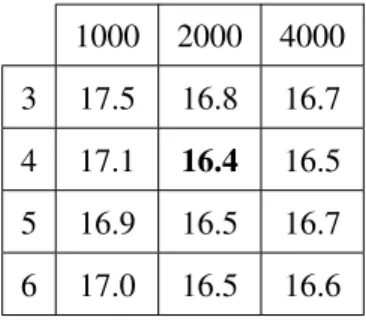
functions, the inputxis a vector. For all others, it is a scalar. . . 26 4.1 Dataset details . . . 48 4.2 Effect of depth and width on DNN TER (development set): This table shows TER
results for DNNs with 1000, 2000, or 4000 hidden units per layer, and 3-6 layers, on the Broadcast News development dataset. All of these models were trained using a linear bottleneck for the output parameter matrix, and using entropy regularized log loss for learning rate decay. The best result is in bold. . . 49 4.3 DNN TER Results (development set): ‘B’ specifies that a linear bottleneck is used,
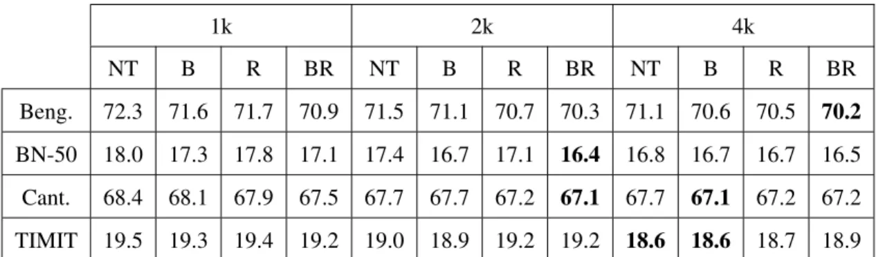
‘R’ specifies that ERP is used (‘BR’ means both are used), and ‘NT’ signifies that neither are used. . . 52 4.4 Kernel TER Results (development set): ‘B’ specifies that a linear bottleneck is used,
‘R’ specifies that ERP is used (‘BR’ means both are used), and ‘NT’ signifies that neither are used. TIMIT models use200krandom features, and all others use100k features. . . 52 4.5 Table of Best DNN vs. Kernel results, across 4 datasets and 5 metrics. . . 53
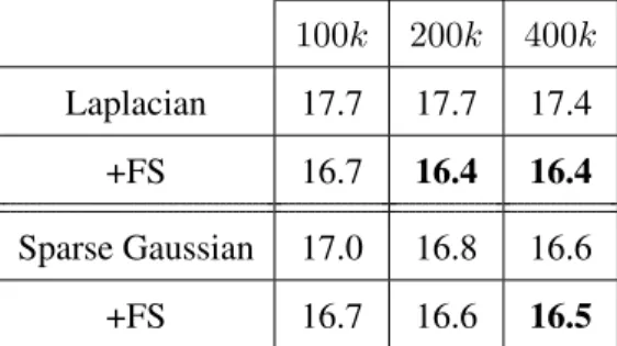
‘R’ specifies that ERP is used (‘BR’ means both are used), and ‘NT’ signifies that neither are used. ‘+FS’ specifies that feature selection was used for the experiments in that row. TIMIT models use200krandom features, and all others use100kfeatures. 61 5.2 Kernel TER Results on Broadcast News development set for models with a very
large number of random feature (up to400k). All models use a bottleneck of size
1000, and use ERP for learning rate decay. . . 62
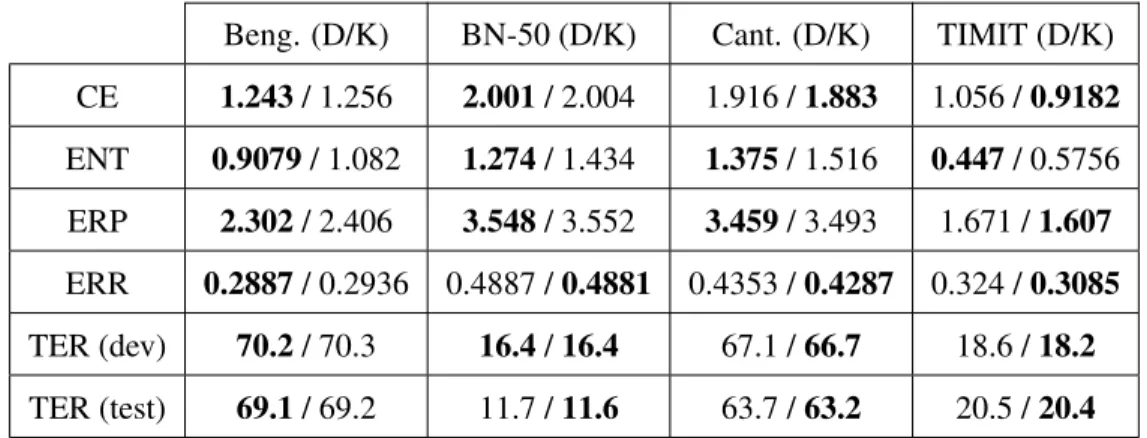
5.3 Table comparing the Best DNN (‘D’) and kernel (‘K’) results, across 4 datasets and 6 metrics. The first 4 metrics are on the heldout set, the fifth is on the development set, and the last metric is reported on the test set. For BN50, the large models from Table 5.2 are included in the set of models from which the best performing model is picked (for each metric). See Section 4.2 for metric definitions. . . 63
5.4 Table comparing the Best DNN and kernel results from this work to those from [Huanget al., 2014] and [Chenet al., 2016], on the TIMIT test set. . . 63
6.1 Dataset details. For classification tasks, we write the number of classes in parenthe-ses in the “task” column. . . 70
6.2 MSE, Bias, and Variance of kernel approximation errorsk(x, y)−z(x)Tz(y)for Nystr¨om (m= 1250), and RFF (m = 20000) features, estimated using many ran-dom pairs of points in the TIMIT heldout set. We partition these pairs of points (x, y)based on whether the true kernel valuek(x, y)is greater than or less than0.25. 77 C.1 DNN: Metric CE . . . 108
C.2 Kernel: Metric CE . . . 109
C.3 DNN: Metric ENT . . . 109
C.4 Kernel: Metric ENT . . . 109
C.5 DNN: Metric ERP . . . 110
C.6 Kernel: Metric ERP . . . 110
C.7 DNN: Metric ERR . . . 110
C.8 Kernel: Metric ERR . . . 111
C.9 Kernel: Metric CE . . . 112
C.11 Kernel: Metric ERP . . . 113 C.12 Kernel: Metric ERR . . . 113 D.1 Hyperparameters used for all datasets . . . 115
First and foremost, I would like to thank my advisor Michael Collins for his years of guidance and valuable feedback. In 2013, when I first met with Mike, I knew very little about machine learning or speech recognition. He brought me from that day to this one. He did this in a number of ways:
1. He immediately gave me a concrete problem to work on. When I first spoke with Mike, he told me about a multi-class classification problem important for speech recognition, and told me to dive right in. This allowed me to get my feet wet right away, and begin to ask the questions necessary to tackle this problem. Little did I know, I would spend the next four years working on it.
2. He was hands-on when necessary. I remember sitting with Mike, working to debug my first implementation of SGD for acoustic model training. It’s not often you hear about an advisor stepping through code with a student.
3. He frequently provided guidance on promising directions to pursue. At so many points during my PhD, Mike has listened to me go through a number of ideas, helping me think about them in new ways, and choose amongst them. He draws from his wealth of knowledge and experience to point me in the most interesting and promising directions. I still remember when he first pointed me to the original random Fourier feature paper.
4. He always provided me with honest feedback. One of the things I most appreciate about Mike is the very clear way in which he presents feedback. By holding my work to his very high standards, and telling me exactly where it currently falls short, he pushes me well beyond where I would be able to get on my own.
5. He gave me the freedom to explore ideas. Often during my PhD, I have spent time studying topics not directly necessary to advance my research, but which I was excited about. Mike
Thank you, Mike, for all the time, energy, and guidance you have given me over the years. You have been instrumental in my reaching this point, and our time together has set the intellectual foundation upon which my future work will build.
I would also like to thank my many collaborators during my time at Columbia. Brian Kingsbury was an invaluable resource. He was instrumental in getting me up and running with all the speech recognition datasets, as well as with all the code necessary to decode the acoustic models I trained. Daniel Hsu has been an important mentor, who helped considerably with the feature selection work in particular. He is always extremely generous with his time, and his insights help me understand the problems I am working on in new ways. Thanks to Fei Sha and his group at USC for our extended collaboration on using random Fourier features for acoustic modeling. It was extremely helpful to have another group with which to discuss ideas, and compare results. The work on Entropy Regularized Perplexity came from their group, and was important for improving the performance of our acoustic models.
During my PhD, I was fortunate to have the opportunity to intern at both Microsoft Research in Redmond, WA, and Google Research in New York City. At Microsoft, I worked with the speech recognition group, and was mentored by Jasha Droppo. At Google, I worked in Sanjiv Kumar’s team, and was mentored by Jeffrey Pennington. Thanks to both groups for welcoming me and teaching me so much.
Prior to beginning my work with Mike, I did research for two years under Professor Augustin Chaintreau. I am deeply indebted to him for all the energy and time he gave me during those two years, and for introducing me to what it really means to do research. I was always impressed by his boundless energy, sharp intellect, and profound kindness and patience. During this time we collaborated closely with Silvio Lattanzi and Nitish Korula at Google Research, two brilliant researchers and kind people from whom I learned a lot.
A special thanks to my PhD committee—David Blei, Shih-Fu Chang, Michael Collins, Daniel Hsu, and Brian Kingsbury—for all the time and energy they have put into reviewing my work, and providing useful feedback and questions.
My time at Columbia would not have been the same without all the friends I made during my time here. Thanks to Karl Stratos for being a close friend and intellectual partner throughout my
for that I am forever indebted. Karl and I spent many hours talking about machine learning (through our “chevruta”), as well as about many other topics (lifestyle, fitness, nutrition, politics, religion, etc.), and I always appreciate hearing his perspective. I admire his love of learning, and endless dedication to self-improvement. Victor Soto has been my officemate and friend for over four years, and has brought much needed levity and companionship to my days. His laughter flows easily, brightening days that would otherwise be quite solitary. Thanks also to Sasha Rush and Yin-Wen Chang for their friendship and mentorship after I joined Mike’s research group, and for their patience with all my questions. Thanks to all my other friends and colleagues at Columbia: Mohammad Rasooli, Erica Cooper, Sarah Ita Levitan, Anna Prokofieva, Andrei Simion, Chris Kedzie, Noura Farra, Tom Effland, Daniel Bauer, Chris Riederer, Arthi Ramachandran, Mathias L´ecuyer, and many others. This ride would have been a lot quieter, and nowhere near as fun, without you all.
I could not have made it to this point without the constant love and support of my entire family. Thanks to both of my sisters, Yael and Orly, for always being there, whether with a helping hand, an empathetic ear, or simply a hug. There are few things I enjoy more than going on runs with them and catching up. Thanks to my brother-in-law Jona and soon-to-be brother-in-law Zev for their friendship, great energy, and for making my sisters happy. And thank you to my niece, Aliza, and my nephew, Benji, for bringing me so much joy every time I see them. And most of all, thank you to my parents, Belly and Ernesto. It’s taken me 30 years to get to this point, and they have been by my side, and rooting for me,everystep of the way. They have taught me by example the importance of putting my full energy behind all of my pursuits, and of always enjoying the ride. There is no way I could ever thank them enough. This work is dedicated to them.
Chapter 1
Introduction
A basic computational problem is to compute an output y ∈ Y based on an input x ∈ X. For example,xcould correspond to a vector of real numbers, andycould correspond to the maximum element in that list. Programming languages provide a medium for precisely expressing the way in whichy should be computed, givenx. However, in many cases, it is very difficult to know, a priori, how to computey, givenx. For example, given a picture, represented by its pixels, how can we compute what is in the picture? Or given an audio recording, how can we predict what words were pronounced? In order to address these challenging scenarios, the field of supervised machine learning takes the following approach: gather as many examples(xi, yi)as possible, define a family
of functionsF fromX toY, and find the functionf∗ ∈ F minimizing some notion of error on the examples you gathered. For example:
f∗= arg min f∈F N X i=1 L(f(xi), yi).
Here,L:Y × Y →Ris a function assigning penaltyL(y0, y)for predicting the labely0 instead of the true labely. Note that ifYis a discrete set, this is calledclassification, whereas ifY ⊆R, this
is calledregression. The goal of thislearningprocess is to find a functionf∗ :X → Ywhich gen-eralizeswell to unseen data; in particular, we would like the expected penaltyEX,Y [L(f∗(X), Y)]
on a random(X, Y)pair to be low.
For a variety of problems, a linear mapping betweenx andy is sufficient. Note that in the context of regression, linear models are defined as the functions of the formf(x) = wTx+b(for somew∈Rd,b∈R), while for binary classification (Y ∈ {−1,+1}), linear models take the form
f(x) = sign(wTx+b), where sign(z) is equal to +1for z ≥ 0, and−1 otherwise. Although the class of linear models might seem overly simplistic, it is quite important. One observation is that linear models can be made very powerful if the feature representation for xis sufficiently expressive.1 However, for many problems, there are no obvious feature representations on top of which a linear function would perform well. For these problems, we must turn to non-linear
methods.
A wide-variety of non-linear methods have been proposed over the years (e.g., decision trees, nearest neighbor methods, etc.). In this thesis, we will focus on two important and powerful families of models: kernel models, and deep neural networks (DNNs). A kernel model is one which makes predictions on a pointxby comparing it with the points in the training set. It does so using expres-sions of the formPNi=1αik(xi, x), where thekernelfunctionk:X × X →Rcan be thought of as a
similarity measure between two points inX. For example, for regression and binary classification, the families of functions considered are:
Freg = {f |f(x) = N X i=1 αik(xi, x) +b, αi∈R}, Fclass = {f |f(x) = sign N X i=1 αik(xi, x) +b , αi ∈R}.
The functions in Freg andFclass can be understood as functions in which all the training points
xi “vote” on what the label should be for a pointx, and these votes are weighted by the
similar-ity betweenxandxi. The set of kernel functionskwhich are generally considered are those that
correspond to a dot-product between points in some Hilbert spaceH, which could be infinite dimen-sional. Specifically,k(x, x0) =hφ(x), φ(x0)iH, whereφ:X → Hmaps a pointxinto the feature
spaceH. As a result, we can understand kernel methods aslinearmethods inH. In particular, for
1
For example, consider learning a binary classifier over a training set of points(xi, yi)whereyi = 1if|xi| ≥ 1,
andyi =−1otherwise. If we usex0i = [xi, x2i]∈R2as the feature representation for theithtraining point, a linear
modely= sign(wTx0+b) = sign(w1x+w2x2+b)would be able to perfectly model this relationship, usingw1= 0,
f ∈ Freg: f(x) = N X i=1 αik(xi, x) +b = h N X i=1 αiφ(xi), φ(x)iH+b = hw, φ(x)iH+b, forw= N X i=1 αiφ(xi)∈ H.
Deep neural networks, on the other hand, computeythrough a combination of linear and non-linear transformations ofx. One common approach is to transformxsequentially, alternating be-tween linear and non-linear transformations. This can be expressed formally by defining the follow-ing class of neural network functions:
F ={f |f(x) =σR(WR·σR−1(...W2·σ1(W1·x+b1) +b2...) +bR)},
where Wi ∈ Rdi×di−1, b
i ∈ Rdi, R ∈ N, and the σ
i : Rdi → Rdi functions are called activa-tion funcactiva-tions, and typically perform an element-wise non-linear transformaactiva-tion of their input. For example, the sigmoid activation function computes 1+expexp(x()x), and the rectified linear unit (ReLU) activation function computesmax(0, x).
Classic results show that both kernel methods and DNNs are “universal approximators,” mean-ing that they can approximate any real-valued continuous function with bounded support to an arbi-trary degree of precision [Cybenko, 1989; Horniket al., 1989; Micchelliet al., 2006]. Thus, some important questions are: Which class of methods performs better on real-world tasks? Which is more efficient, in terms of training time, test time, and in terms of memory requirements? Are there learning algorithms for each of these model families which are guaranteed to return the optimal f∗∈ F?
Training a kernel model corresponds to solving a convex optimization problem, and thus there exist techniques which find the optimalf∗∈ F. Unfortunately, these methods typically do not scale well to large datasets. In particular, with data sets of sizeN, theΘ(N2) size of the matrixK of pairwise kernel values (Kij =k(xi, xj)) makes training prohibitively slow, while the typicalΘ(N)
size of the resulting models [Steinwart, 2004] makes their deployment impractical. Thus, kernel methods are typically not applied to very large-scale problems, with millions of training points.
'00 '04 '12 '17 5
10 20 30
Word Error Rate (%)
Switchboard Performance (2000-2017) 19.3 14.8 13.3 5.5 GMMs Deep Learning Machine Human (MSFT) Human (IBM) ImageNet Winners (2010-2017) 28.2 25.8 16.4 11.7 6.7 3.6 3.0 2.3 Deep Learning '10 '11 '12 '13 '14 '15 '16 '17 0 5 10 15 20 25 30 35
ImageNet Top-5 Error Rate (%)
Machine Human
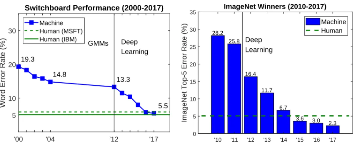
Figure 1.1: Impact of deep learning methods on state of the art performance in speech recognition and computer vision.
In contrast, DNNs are able to scale gracefully to very large datasets. They are generally trained using stochastic gradient methods, meaning that at each iteration of the algorithm, the parameters are updated using an unbiased estimate of the full gradient, which is obtained by computing the objective function on a random sample of training points. Unfortunately, the training objective for DNNs is non-convex, and thus it is generally impossible to guarantee that the model returned by the training algorithm is optimal. Nonetheless, in recent years, deep learning techniques have significantly advanced state of the art performance in various domains, including automatic speech recognition (ASR) [Seideet al., 2011a; Hintonet al., 2012; Mohamedet al., 2012; Saonet al., 2017; Xionget al., 2017], computer vision [Krizhevskyet al., 2012; Simonyan and Zisserman, 2014; He
et al., 2016], and natural language processing (NLP) [Mikolovet al., 2013; Sutskeveret al., 2014; Andoret al., 2016]. In Figure 1.1, we show the impact of deep learning methods on state of the art performance in speech recognition and computer vision. As you can see, in the past 5 years or so, deep learning methods have achieved impressive performance gains in both of these settings.2
The primary focus of this thesis is answering the following question:
Can kernel methods be scaled to compete with DNNs in the large-scale settings in which DNNs currently dominate?
2Importantly, the Switchboard task is a relatively easy one; it consists of clear, unaccented speech between strangers,
In particular, we will focus on theacoustic modeling problem in speech recognition, which is the problem of modeling the pronunciation of the basic phonetic units of speech. Specifically, for a given frame of audio (typically corresponding to 25 ms), we must model the probability that the frame corresponds to a specific meaningful unit of speech. In the simplest setting, the set of units considered are calledphonemes, which are the smallest units of sound which distinguish one word from another in a given language (for example, ‘/b/’ and ‘/p/’ correspond to different phonemes, because they distinguish the words “bark” and “park” from one another).3 However, because the pronunciation of a phoneme is very affected by the phonemes that come before and after it, it is very beneficial to model phonemes in context. In order to address the very large number of context-dependent phoneme states (Sc if there are S phonemes, and a context window of size c is used), these states are clustered using decision trees [Hwanget al., 1993; Young et al., 1994]. These clustered states are called senones, and there are typically thousands of them, presenting a scalability challenge for training acoustic models.
Deep learning techniques have significantly advanced the state of the art in acoustic modeling, by modeling the probabilityp(y|x)that an acoustic framex(represented as a vector inRdof
acous-tic features) corresponds to a senoney. In this thesis, we will scale kernel methods to this problem usingapproximationtechniques, which help bypass the computational expense of solving the kernel method exactly. Much recent effort has been devoted to the development of approximations to ker-nel methods, primarily via the Nystr¨om approximation [Williams and Seeger, 2001] and via random feature expansion (e.g., [Rahimi and Recht, 2007; Kar and Karnick, 2012]). These methods yield explicit feature representations on which linear learning methods can provide good approximations to the original non-linear kernel method. Specifically, they provide ways of generating representa-tionsz(x)∈RD such thathz(x), z(y)i ≈k(x, y). By reducing the time and memory requirements
to beinglinearin the size of the training set, these methods unlock the potential of applying kernel methods to truly large-scale tasks. However, there have been very few published attempts applying these methods to the challenging large-scale tasks on which deep learning techniques have truly shined (see Related Work section for discussion).
3
Note that we distinguish phonemes from letters by using the ’/’ notation; ‘b’ is a letter, while ‘/b/’ corresponds to the sound one makes when pronouncing the letter ‘b.’ Note that some letters can be pronounced multiple ways, making this an important distinction.
The primary contribution of this thesis is to demonstrate that kernel approximation methods can effectively compete with fully-connected feedforward neural networks on the acoustic modeling task. More specifically:
• We benchmark the performance of randomized kernel features relative to fully-connected DNNs on the acoustic modeling problem. Specifically, we use random Fourier features [Rahimi and Recht, 2007], and report results on four datasets.4
• We propose a novel feature selection method which can significantly improve the perfor-mance of a kernel model trained on a fixed number of random Fourier features. We show that using this technique, kernel methods effectively match the performance of feedforward DNNs across the four datasets.
• We perform an in-depth analysis comparing the performance of random Fourier features with the Nystr¨om method for kernel approximation, in the large-scale setting. We compare these representations in terms of their kernel approximation error, their memory requirements, and their performance when used for learning.
This contribution is important for both practical and theoretical reasons. From a practical per-spective, it suggests that randomized features can be competitive with deep learning methods on large-scale tasks. From a theoretical perspective, it adds to our understanding of DNNs and non-linear classification. There is a large open question of why DNNs work, which is being actively investigated from various directions, including optimization [Dauphin et al., 2014; Choroman-skaet al., 2015; Anandkumar and Ge, 2016; Agarwalet al., 2017; Xieet al., 2017; Pennington and Bahri, 2017], representational power and efficiency [Cybenko, 1989; Hornik et al., 1989; Bengio and Lecun, 2007; Bianchini and Scarselli, 2014; Mont´ufar et al., 2014; Ba and Caruana, 2014], and generalization performance [Bartlett, 1996; Neyshaburet al., 2015; Zhanget al., 2017; Arpitet al., 2017]. The fact that a shallow architecture with random features can match DNNs on a task this large and challenging gives an important new perspective.
This thesis is organized as follows: Chapter 2 provides background on kernel methods, kernel approximation methods, deep neural networks, speech recognition, and acoustic modeling. We
4
We use the IARPA Babel Program Cantonese (IARPA-babel101-v0.4c) and Bengali (IARPA-babel103b-v0.4b)
review related work in Chapter 3. In Chapter 4, we present our work benchmarking the performance of random Fourier features relative to DNNs on four speech datasets. In Chapter 5 we present our feature selection algorithm, along with extensive experimental results using this method. In Chapter 6 we present our work comparing the Nystr¨om method with random Fourier features. Lastly, we present our conclusions, and discuss directions for future work, in Chapter 7.
The work presented in Chapters 4 and 5 is a much extended version of the paper titled “Compact Kernel Models for Acoustic Modeling via Random Feature Selection” [May et al., 2016]. These chapters also extend joint work with Luet al. titled “A Comparison Between Deep Neural Nets and Kernel Acoustic Models for Speech Recognition” [Luet al., 2016]. This extended work has been posted publicly as a pre-print [Mayet al., 2017], which is the primary document from which these chapters are adapted.
Chapter 2
Preliminaries
In this chapter, we provide background on kernel methods, kernel approximation, deep neural net-works, and speech recognition. We begin by discussing the notation which we will use throughout this thesis. As further background, we include a number of important mathematical definitions in Appendix A (metric spaces, Hilbert spaces, Cauchy sequences, positive definite functions/matrices, etc.).
2.1
Notation
We will use the following notation throughout the thesis:
• Rwill denote the real numbers,Cthe complex numbers, andNthe natural numbers.
• [n]will denote the set{1,2, . . . , n}. Ifnis infinite, then[n] =N.
• kwill denote thousands, andM will denote millions (e.g.,100kwill denote100thousand, and2M will denote 2 million).
• We will use lower case letters to denote vectors (e.g.,x), and we will usexi to indicate the
ithelement of the vectorx∈Rd. By default, vectors will be assumed to be column vectors.
• We will use capital letters to denote matrices (e.g.,A), and useAij to indicate the element in
theithrow andjthcolumn ofA.
• C=A◦Bwill denote the Hadamard product between two matricesAandB, also known as the element-wise product (Cij =AijBij).
• xT will denote the transpose of a vectorx, andAT will denote the transpose of a matrixA. • kAkF will denote the Frobenius norm of a matrixA, andkAk2 will denote its spectral norm. • 0dwill denote thed-dimensional zero vector, and0will denote the zero element in a vector
spaceX.
• 1N,N will denote theN×N identity matrix.
• X will denote the space of inputs, andY will denote the space of outputs (typically equal to
Ror[c]for somec∈N).
• k:X × X →Rwill denote a kernel function, andK ∈RN×N will denote the kernel matrix
for a specific training set{x1, . . . , xN} ⊂ X, withKij =k(xi, xj).
• H will denote the feature space associated with a kernel function k, or more formally, its Reproducing Kernel Hilbert Space (see Section 2.4 for the definition).
• hx, x0iHwill denote the inner-product in a spaceHbetweenxandx0. IfHis not specified,
andx, x0 ∈ RD, we can assume the standard dot-producthx, x0i = PD
i=1xix0i is used. In
this case, we will often write this dot product asxTx0. Ifx, x0 ∈ CD, we use the standard
complex dot-product: hx, x0i = PD
i=1xix0i, where adenotes the complex conjugate of any
a∈C.
• kxkH=
p
hx, xiHwill denote the norm of a vector in a Hilbert spaceH. IfHis not specified,
andx∈RD, we can usekxk1 =Pi|xi|to denote the`1norm ofx, andkxk2=qPix2i to denote the`2norm ofx, also known as the Euclidean norm.
2.2
Kernel methods
Kernel methods, broadly speaking, are a set of machine learning methods which learn to make predictions on unseen datapoints by considering their similarity to the points in the training set. In general, we define the similarity between two points inX through a kernel functionk:X ×X →R.
Kernel models make predictions on unseen points x by making use of expressions of the form h(x) = PNi=1αik(xi, x) +b; for regression, h(x)is used directly as the prediction of the model
f(x), while for binary classification,f(x) = sign(h(x)). Thus, each training pointsxican influence
the prediction of the modelfon a pointx, where this influence is weighted by the similarity between xiandx. If the kernel functionk(x, x0)corresponds to a dot-producthφ(x), φ(x0)iHin some feature
spaceH, then we can additionally interpret kernel models as linear models in this space: h(x) = N X i=1 αik(xi, x) +b = * N X i=1 αiφ(xi), φ(x) + H +b = hw, φ(x)iH+b, forw= N X i=1 αiφ(xi).
Here, φ : X → H is a feature map which sends a point in X to its corresponding point in H. Importantly, for all positive definite kernelsk, such a map exists.1 Thus, kernel methods can be seen
as a set of machine learning techniques which either explicitly (withφ) or implicitly (withk) map data from the input spaceX to some Hilbert spaceH, in which a linear model is learned. We will now discuss the two primary ways of understanding kernel methods in more detail, corresponding to whether this mapping toHis explicit or implicit. In this discussion, we will usedto denote the dimension ofX, Dto denote the dimension ofH(which could be infinite), andN to denote the number of training points(xi, yi).
2.2.1 Primal formulation
In the first formulation (which we will call the “primal”), we consider anexplicitmappingφ:X → H. We then learn a linear model directly on these representations:
w∗= arg min w∈H,b∈R N X i=1 L(hw, φ(xi)iH+b, yi) +R(w). 1
In fact, there are many such maps, which are all equivalent (i.e., isometrically isomorphic), yet take very different
forms. One such map is the mapping fromxto the functionk(x,·)in the Reproducing Kernel Hilbert Space fork(see
Section 2.4). Another is given by Mercer’s Theorem, which shows that such a map exists, where the dimension of the
spaceHis countably infinite [mer, 1909]. Yet another is given by Bochner’s Theorem, in the case ofshift-invariant
Here,R(w)is a regularization term which encourages simple models (typically, by penalizing the norm ofw; for example,R(w) = λ2kwk2
H), in order to improve generalization performance ofw∗.
Additionally, L : R× Y → R is a generic loss function, which penalizes the model based on
some function ofhw, φ(xi)iH+band the true labelyi. The setYcorresponds toRfor regression,
and{−1,+1}for binary classification. For regression, the quadratic lossL(zi, yi) = 12(zi −yi)2
is typical, while for binary classification, the cross-entropy loss function L(zi, yi) = log (1 +
exp(−yizi)
is common.
As an example, consider the following feature map φ : R2 → R5, applied to a point x =
[x1, x2]∈R2: φ(x) = (x21, x22,√2x1x2, √ 2x1, √ 2x2,1). (2.1)
A linear model trained on top of this feature representation would in effect be finding the optimal quadratic function for the given task. This demonstrates how learning a linear model over features generated through a non-linear mapφ:X → Hcorresponds to learning a non-linear model in the original spaceX. This can imbue the model with a lot more power.
For a given map φ, we can define the corresponding kernel function k : X × X → R as k(x, x0) =hφ(x), φ(x0)iH. For example, in the case of the quadratic mapφshown in Equation 2.1,
the corresponding kernel function is
k(x, x0) =x21x102+x22x022+ 2x1x2x01x02+ 2x1x01+ 2x1x01+ 1 = (xTx0+ 1)2
(2.2)
Importantly, definingk(x, x0)as a dot-product in some spaceHimplies thatkis a positive definite function, meaning that for anyc1, . . . , cN ∈R, and anyx1, . . . , xN ∈ X,PNi,j=1cicjk(xi, xj)≥0.
This is easy to see, becausePNi,j=1cicjk(xi, xj) =hPNi=1ciφ(xi),PNi=1ciφ(xi)iH≥0.
It is important to note that the computational expense of performing one epoch of stochastic gradient descent on the primal optimization problem discussed above isO(N D)(Recall,N is the size of the training set, andDis the dimension ofH. Here we do not include the cost of computing φ(x).). This is fast as long as neitherN orDis too large. Unfortunately, for a wide variety of of kernels, Dis extremely large, or even infinite. In order to address this computational hurdle, we can instead work with the dual formulation of the optimization problem; this is discussed in the following section.
2.2.2 Dual formulation
In the second formulation (which we will call the “dual”), instead of defining the kernel functionk in terms of an explicit mapφ, we instead define the kernel functionk:X × X → Rdirectly. We require thatkbe a positive definite function. Generally, we can think ofkas a similarity function, which will assign a high score to pairs of points that are similar (e.g., close inRd), and a low score
to points that are different. For example, we list some common kernel functions in Table 2.1. Gaussian kernel: k(x, x0) = exp
−kx−x0k22
2σ2
Laplacian kernel: k(x, x0) = exp−λkx−x0k1 Polynomial kernel (degreer): k(x, x0) = (xTx0+ 1)r
Table 2.1: A few example kernel functions.
As you can see, the kernel we defined in Equations 2.1 and 2.2 is an example of a degree 2 polyno-mial kernel. Notice that for all of these kernels, the kernel function can be computed inO(d), where dis the dimension ofX.
We saw above how to perform optimization in the primal view of the problem. But how do we learn models using the dual view? For a large set of primal optimization problems of the form
w∗= arg min w∈H,b∈R N X i=1 L(hw, φ(xi)iH+b, yi) +R(w),
it is possible to reformulate the problem as an equivalentdualoptimization problem, which only requires knowledge of the kernel matrixK∈RN×N. For example, the SVM primal problem is:
min w∈H,b∈R C N X i=1 max 0,1−yi hw, φ(xi)iH+b+kwk2H.
The corresponding dual problem is: max αi≥0 N X i=1 αi− 1 2 N X i,j=1 αiαjyiykk(xi, xj)
subject toαi ∈[0, C]∀i, and N
X
i=1
αiyi= 0.
After the optimal dual parameters α∗i are found by solving the above optimization problem, the optimal bias termb∗ can be computed by taking any vectorxj for which0 < α∗j < C (these are
called “support vectors”), and solving for b∗ in the equation 1 = yj(PNi=1α∗iyik(xi, xj) +b∗).
Then, the model corresponding to these parameters isf(x) = sign(PNi=1αi∗yik(xi, x) +b∗).
Importantly, the dual optimization problem interacts with the datapointsxiexclusively through
the kernel functionk. Importantly, both the primal and the dual optimization problems for kernel methods are convex. In the case where the kernel functions between two points can be computed quickly (e.g., inO(d)), and the dimension Dof the primal space His much bigger thanN, it is more efficient to solve the dual (time at least quadratic inN) than to solve the primal (time at least linear inN D). This is called the “kernel trick,” and it allows us to find the optimal linear classifier inH, even if it is an infinite dimensional space. However, ifN is very large, the dual formulation will be too expensive to solve as well, as it requires performing an optimization over the fullN×N kernel matrix; simply computing the kernel matrix takes time(N2d)(assuming kernel evaluations takeO(d)). As an example, for a dataset with a million training points, the kernel matrix consumes four terabytes of memory if stored as single precision floats. This leads to the following question: What can we do in the case where bothN andDare extremely large? For example, what ifDis infinite, andN is in the millions? In this case, one can use kernel approximation methods, which we now discuss.
2.3
Kernel approximation
In the section, we discuss two important ways of doing kernel approximation: random Fourier features [Rahimi and Recht, 2007], and the Nystr¨om method [Williams and Seeger, 2001]. These methods share the following goal: to construct low-dimensional representationsz(x) ∈ RD such
thatz(x)Tz(x0)≈k(x, x0). We can then simply train a linear model on top of these representations in order to attain an approximate solution to the exact kernel optimization problem. Training would thus requireO(N D)time per epoch,2 which is much better than solving the dual problem when D << N. In particular, for a fixedDthis runtime only growslinearlyinN, making this appealing in the large-scale setting. We now provide overviews for how z(x) is constructed, using either
2
This runtime assumes thatz(x)can be computed inO(D)for everyx, which is generally not the case. However,
even if computingz(x)is more expensive than this, you can incur this as a one-time cost at the beginning of training, and
store the representationsz(x)to disk (or in memory). If we assume computingz(x)isO(Dd), which is common, and
random Fourier features, or the Nystr¨om method.
2.3.1 Random Fourier features (RFF)
For the random Fourier features method [Rahimi and Recht, 2007], the theorem which allows for the construction of the representationz(x)is called Bochner’s Theorem. This is a classical result in harmonic analysis, and it allows us to approximate any positive-definiteshift-invariantkernelkwith
finite-dimensional features. A kernelk(x, x0)isshift-invariantif and only ifk(x, x0) = ˆk(x−x0) for some functionkˆ:Rd→R. We now present Bochner’s Theorem:
Theorem 1. (Bochner’s Theorem, adapted from [Rahimi and Recht, 2007]): A continuous
shift-invariant kernel k(x, x0) = ˆk(x−x0) on Rd is positive-definite if and only if kˆ is the Fourier
transform of a non-negative measureµ(ω).
Thus, for any positive-definite shift-invariant kernelk(δ), we have thatˆ ˆ k(δ) = Z Rd µ(ω)e−jωTδdω, (2.3) where µ(ω) = (2π)−d Z Rd ˆ k(δ)ejωTδdδ (2.4) is the inverse Fourier transform3 ofˆk(δ), and wherej = √−1. By Bochner’s theorem, µ(ω) is a non-negative measure. As a result, if we letZ = R
Rdµ(ω)dω, thenp(ω) =
1
Zµ(ω)is a proper
probability distribution, and we get that 1
Zˆk(δ) =
Z
Rd
p(ω)e−jωTδdω.
For simplicity, we will assume going forward thatkˆ is properly-scaled, meaning thatZ = 1. Now, the above equation allows us to rewrite this integral as an expectation:
ˆ k(δ) = ˆk(x−x0) = Z Rd p(ω)ejωT(x−x0)dω=Eω h ejωTxe−jωTx0i. (2.5) This can be further simplified as
ˆ
k(x−x0) =Eω,b
h√
2 cos(ωTx+b)·√2 cos(ωTx0+b)i,
3
There are various ways of defining the Fourier transform and its inverse. We use the convention specified in Equations (2.3) and (2.4), which is consistent with [Rahimi and Recht, 2007].
Kernel name k(x, x0) p(ω) Density name Gaussian e−kx−x0k2 2/2σ2 (2π(1/σ2))−d/2e− kωk2 2 2(1/σ)2 Normal(0 d,σ121d,d) Laplacian e−λkx−x0k1 Qd i=1 λπ(1+(1ωi/λ)2) Cauchy(0d, λ) Table 2.2: Gaussian and Laplacian Kernels, together with their sampling distributionsp(ω)
whereω is drawn fromp(ω), andbis drawn uniformly from [0,2π]. See Appendix B for details on why this specific functional form is correct.4 In Table 2.2, we list two popular (properly-scaled) positive-definite kernels with their respective inverse Fourier transformsp(ω).
This motivates a sampling-based approach for approximating the kernel function. Concretely, we draw{ω1, ω2, . . . , ωD}independently from the distributionp(ω), and{b1, b2, . . . bD}
indepen-dently from the uniform distribution on[0,2π], and then use these parameters to approximate the kernel, as follows: k(x, y) ≈ 1 D D X i=1 √ 2 cos(ωiTx+bi)· √ 2 cos(ωiTy+bi) = z(x)Tz(x0), wherezi(x) = q 2
Dcos(ωiTx+bi) is theith element of theD-dimensional random vectorz(x).
This gives us the explicit (random) mappingz:Rd→RD proposed by the random Fourier features
method. It has the very nice property that for all indicesi ∈[D],Eω,b[zi(x)zi(x0)] = D1k(x, x0),
and thus thatEω,b
z(x)Tz(x0)=k(x, x0).
We can bound the probability that z(x)Tz(x0) is more than away from k(x, x0) as follows. First, defineXi = q 2 Dcos(ω T i x+bi) q 2 D cos(ω T i x 0+b
i)to be a random variable corresponding
to random draws ωi, bi, and let X = PDi=1Xi. Noticing that Xi ∈ [−D2,D2], that Eω,b[X] =
k(x, x0), and that X = z(x)Tz(x0) for the random representations z(x), z(x0), we can directly apply Hoeffding’s inequality onXto prove the desired bound:
Pω,b |z(x)Tz(x0)−k(x, x0)| ≥≤2 exp −D2 8 . (2.6) 4
Another important thing to notice is that the integral in Equation 2.5 immediately gives us an explicit mappingφ
fromX =Rdto the space of complex square-integrable functionsL2(Rd, p), whereφ(x)is the functionfx :Rd→C
defined asfx(ω) =eω Tx . Thus,hφ(x), φ(x0)iL2 = R Rdfx(ω)fx0(ω)p(ω)dω= R Rdp(ω)e jωT(x−x0) dω =k(x, x0), as desired. See Section D.4.1 in Appendix D for more details on how this Hilbert space is defined.
In the original work by Rahimi and Recht, the authors prove a much stronger result, bounding the probability thatz(x)Tz(x) is within ofk(x, x0)for all pairsx, x0 ∈ X simultaneously[2007]. Specifically, they show that ifD = ˜Ω(d2), then with high probabilityz(x)Tz(x
0)will be within
ofk(x, x0) forall x, x0 in some compact subset M ∈ Rd of bounded diameter.5 See Claim 1 of
[Rahimi and Recht, 2007] for the more precise statement and proof of this result.
In their follow-up work, Rahimi and Recht prove a generalization bound for models learned using these random features [2008]. They show that with high-probability, the excess risk6assumed from using this approximation, relative to using the “oracle” kernel model (the exact kernel model with the lowest risk), is bounded byO(√1
N+
1
√
D)(see the main result of [Rahimi and Recht, 2008]
for more details). Given that the generalization error of a model trained using exact kernel methods is known to be withinO(√1
N) of the oracle model [Bartlettet al., 2002], this implies that in the
worst case, D = Θ(N)random features may be required in order for the approximated model to achieve generalization performance comparable to the exact kernel model. Empirically, however, fewer thanΘ(N)features are typically needed in order to attain strong performance, as we will see in Chapters 4, 5, and 6, and as has been seen in existing work (e.g., [Yuet al., 2015]).
2.3.2 Nystr¨om method
Like random Fourier features, the Nystr¨om method constructs a feature representationz(x) ∈ RD
such thatz(x)Tz(x0)≈k(x, x0). However, the Nystr¨om method takes an entirely different approach in order to construct this feature map. Instead of finding a way to approximate k(x, x0) well for any pair x, x0 ∈ X, the Nystr¨om method approaches this problem from the perspective of low-rank matrix decomposition. Specifically, the Nystr¨om method attempts to approximate the full kernel matrixKwell (e.g., in terms of Frobenius or spectral norm), using a low-rank decomposition
ˆ
K =ZTZ, where theithcolumn ofZ will correspond toz(x
i). Note that one can find the optimal
suchZ ∈ RD×N minimizing bothkK−ZTZk
F as well askK−ZTZk2 by taking the singular value decomposition (SVD)K = UΛUT of the kernel matrixK (with the singular values sorted
from largest to smallest along the diagonal of Λ); then, the optimal ZT = UDΛ1D/2, where ΛD
denotes theD×Ddiagonal matrix of the Dlargest singular values, and UD denotes the firstD 5We are using theΩ˜notation to hide logarithmic factors.
6
columns ofU (which correspond to the singular vectors of the largest singular values). There are two problems with this solution:
1. Computing the SVD of aN ×N matrix takesO(N3), and is thus impractical for very large N, which is precisely the setting in which we are interested in using kernel approximation. Given that we can generally solve the dual kernel optimization problems inO(N3), there is no reason to prefer this method from an efficiency perspective.
2. From the above definition forz(x), it is not clear how one would computez(x)for a pointx which isn’t in the training set.7This however, has an easy solution; if we letAD =UDΛ
−1/2 D , we get: KAD = KUDΛ −1/2 D = (UΛUT)UDΛ −1/2 D = UDΛDΛ −1/2 D = ZT. Thus, if we let ZT = KA D, we can take z(x) = ATDkx = Λ −1/2 D UDTkx, where kx =
[k(x, x1), . . . , k(x, xN)]T is the vector of kernel evaluations betweenxand all training points
xi. Notice that this function z(·) ∈ span(k(x1,·), . . . , k(xN,·)) ⊂ H, and thus a
lin-ear model trained on top of this representation automatically gives us a model of the form
PN
i=1αik(xi,·), which we will see in Section 2.4.1 must be the form of the optimal kernel
model (by Representer Theorem). Note, however, that while this solves the problem of how to computez(x)∈RD for any pointx∈ X, it does not address the computational issue, that
computingAD still requires taking the SVD of the full kernel matrixK.
The Nystr¨om method addresses the first problem raised above, by taking inspiration from the so-lution to the second problem. The intuition behind the Nystr¨om method is as follows: instead of constructing the representation z(x) based on the SVD of the full kernel matrix K, consider in-stead the SVD ofKm,m, the kernel matrix corresponding to “landmark” points{ˆx1, . . . ,xˆm}; note
that normally, these landmark points are selected from the training set (e.g., uniformly at random),
7
but this need not be the case (e.g., [Zhanget al., 2008]). Now, we can considerz(x) = ˆATDkˆx,
where Km,m = ˆUΛ ˆˆUT is the SVD of the landmark point kernel matrix, AˆD = ˆUDΛˆ
−1/2
D , and
ˆ
kx= [k(x,xˆ1), . . . , k(x,xˆm)]T. TakingZm = [z(ˆx1), . . . , z(ˆxm)]as theD×mmatrix withz(ˆxi)
as theithcolumn, gives us the optimal rankDdecompositionZmTZmforKm,m, as discussed above
(ZmTZm = Km,m if m = D). However, we can take this z(x) ∈ RD to be our representation
for any point x ∈ X, and this gives us a low rank decompositionZTZ to the full kernel matrix K, whereZ = [z(x1), . . . , z(xN)]. Thisz(x) is precisely the representation which the Nystr¨om
method constructs for the purposes of kernel approximation. Just like with random Fourier features, one can learn a linear model on top of these representations in order to approximately solve the kernel optimization problem.
One important thing to note is the cost of the Nystr¨om method, both in terms of time and memory:
1. Time (SVD): Computing the SVD of them×mkernel matrix takesO(m3). Note that when D < m, the SVD can be done faster using randomized SVD algorithms [Halkoet al., 2011], which would takeO(m2D)instead ofO(m3).
2. Time (training): During training, we must compute the representation z(x) = ˆATDkˆx for
every training pointx. Assuming computingk(x, x0) takes timeO(d)for x, x0 ∈ Rd, this
takes timeO(N md+N mD). This is because computingˆkxi ∀itakes timeO(N md), while computing the matrix multiplicationAˆTDˆkxitakesO(N mD)(O(mD)cost for eachxi). Note that this is a lot more expensive than the cost of random Fourier features, which take time O(N Dd) ≤ O(N mD) to compute; importantly, for RFF this can be further reduced to O(N Dlog(d))using structured matrix multiplications [Leet al., 2013; Yuet al., 2015]. 3. Memory: Storing the m landmark points requires storing mdfloats, while storing theAˆD
matrix requiresmDstorage. This brings the total memory requirement toO(md+mD). Note that this is substantially more expensive than the storage costs of random Fourier features, which simply requireO(Dd) ≤ O(md), and which can be further reduced toO(D)[Leet al., 2013; Yuet al., 2015].
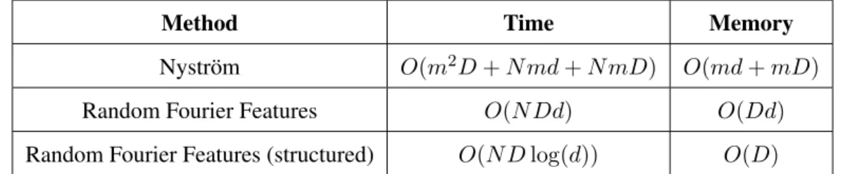
In Table 2.3, we summarize the computational costs of Nystr¨om vs. random Fourier features, dis-cussed above.
Method Time Memory
Nystr¨om O(m2D+N md+N mD) O(md+mD)
Random Fourier Features O(N Dd) O(Dd)
Random Fourier Features (structured) O(N Dlog(d)) O(D)
Table 2.3: Cost of computing Nystr¨om vs. random Fourier features (RFF), both in terms of time and memory. For RFF, we also report the costs of the more efficient implementation using structured matrices [Leet al., 2013; Yuet al., 2015].
There are a variety of ways of understanding the Nystr¨om method, aside from the one explained above. They include:
1. As a projection onto a subspace.
2. As a solution to an optimization problem. 3. As a preconditioning method.
4. As a way to approximate the eigenvalues and eigenfunctions of the linear operator of the kernel function, using Monte Carlo approximation.
These are all explained in further detail in Appendix D.
2.4
Reproducing kernel Hilbert spaces (RKHS)
One way of understanding kernel methods is as optimization over a space of functions from X to R. The space of functions which corresponds to a specific kernel is called its Reproducing
Kernel Hilbert Space (RKHS). Given a symmetric positive definite kernel k : X × X → R, its corresponding RKHS is essentially defined as the set of all linear combinations of functions of the formk(x,·), forx∈ X. Note that here I am using the notationk(x,·)to correspond to the function fx:X →Rsuch thatfx(x0) =k(x, x0).
There are several ways of formally defining an RKHS [Sejdinovic and Gretton, 2012]; in this section, however, we will focus on the Moore-Aronsajn construction of the RKHS corresponding to a positive definite kernelk[Aronszajn, 1950]. This construction has two main steps: first, we
will define the “pre-RKHS”H0 as the set of allfinitelinear combinations of functions of the form k(x,·)forx∈ X. Note that this is a subset ofRX, the space of all functions fromX toR. We will
then turn this into acompletespaceHby adding toH0the set of all its limit points inRX. We now
go through both of these steps in detail.
We begin by defining the setH0, along with an inner product in this space: H0={f(·) =
n
X
i=1
αik(xi,·)|xi∈ X, αi∈R, n∈N}.
We now define the inner product betweenf =Pni=1αik(xi,·)andg=Pmj=1βjk(˜xj,·)inH0as: hf, giH 0 = n X i=1 m X j=1 αiβjk(xi,x˜j).
Now, if we consider the functionφ:X → H0, defined asφ(x) =k(x,·), we can see by the above definition thathφ(x), φ(x0)iH0 =hk(x,·), k(x
0,·)i
H0 =k(x, x
0). Thus, we have constructed a map
φto a space H0 in which k(x, x0) = hφ(x), φ(x0)iH0, allowing us to view optimization over an
RKHS as searching for a linear model in this space.8
Note that the above definition of the inner product in H0 implies that the (squared) norm of a functionk(x,·) ∈ H0 iskk(x,·)kH20 = hk(x,·), k(x,·)iH0 = k(x, x). Furthermore, using this
definition we can show that the “reproducing property” holds in H0—namely, that for any f =
Pn
i=1αik(xi,·)∈ H0, and anyx∈ X,hf, k(x,·)i=f(x). This can be seen easily: hf, k(x,·)i = * n X i=1 αik(xi,·), k(x,·) + H0 = n X i=1 αik(xi, x) = f(x).
If we are in the case where we have an explicit feature map φ : X → H0, we can view the
8
corresponding pre-RKHSH0as follows: H0 = {f(·) = n X i=1 αik(·, xi)|xi ∈ X, αi ∈R, n∈N} = {f(·) = n X i=1 αihφ(·), φ(xi)iH0 |xi∈ X, αi∈R, n∈N} = {f(·) = * φ(·), n X i=1 αiφ(xi) + H0 |xi ∈ X, αi ∈R, n∈N} = {fa(·) =hφ(·), aiH0 |a= n X i=1 αiφ(xi), xi∈ X, αi∈R, n∈N}.
Thus, each function in H0 can be associated with a unique element a ∈ H0. Furthermore, we will now show that the dot-product between two elements in H0 corresponds to the dot-product between the corresponding points in H0. For fa, fb ∈ H0, where fa = Pni=1αik(·, xi), fb =
Pm
j=1βjk(·,x˜j), and the corresponding points a = Pni=1αiφ(xi) and b = Pmj=1βjφ(˜xj), we
have: hfa, fbiH0 = n X i=1 m X j=1 αiβjk(xi,x˜j) = n X i=1 m X j=1 αiβjhφ(xi), φ(˜xj)iH0 = * n X i=1 αiφ(xi), m X j=1 βjφ(˜xj) + H0 = ha, biH0
This shows that there is a very strong correspondence between the spaceH0 and the subspace of the feature spaceH0composed of all finite linear combinations of pointsφ(x)forx∈ X. In fact, these spaces are isometrically isomorphic, meaning that there exists a linear bijection ψbetween the spaces, and this map preserves inner products (hf, giH0 =hψ(f), ψ(g)iH0). This map takes the
expected form, mappingfa∈ H0toa∈ H0.
In order to turn this pre-RKHS H0 into a proper Hilbert space H ⊃ H0, we need to make it
complete; this means that all Cauchy sequences in Hmust converge to points inH. Specifically, we must add toH0the pointsf ∈RX for which there exists a Cauchy sequence{f1, f2, . . .} ∈ H0 which converges pointwise tof. Given two such points,f andg, wheref is the limit of the
Cauchy-sequence{fn}, andgis the limit of{gn}, we define the dot product betweenf andgas the limit of
the dot products of the sequences:hf, giH= limn→∞hfn, gniH0.
For more of the formal mathematical details behind this construction, see [Berlinet and Thomas-Agnan, 2003; Sejdinovic and Gretton, 2012].
2.4.1 Representer Theorem
One very important result regarding optimization over an RKHS is the Representer Theorem, which we present now:
Theorem 2. (Representer Theorem, adapted from [Sch¨olkopfet al., 2001]): Letk :X × X → R
be a symmetric positive definite kernel, andH its RKHS. Then, for any non-decreasing function
G : R → R, any loss function L : (X × Y ×R)N → R∪ {+∞}, and any N labeled points
(xi, yi)∈ X × Y, the optimization problem
arg min
f∈H
G(kfkH) +L((x1, y1, f(x1)), . . . ,(xN, yN, f(xN)))
has a solution of the formf∗ =PNi=1αik(xi,·). Furthermore, ifGis a strictly increasing function,
then any solution has this form.
Proof. LetA = span(k(x1,·), . . . , k(xN,·)) ⊂ H, and letA⊥be the orthogonal complement of
AinH. Thus,H=A⊕A⊥, and anyf ∈ Hcan be uniquely decomposed asf =fA+fA⊥, for
fA ∈ AandfA⊥ ∈A⊥. It follows from the reproducing property, and the orthogonality between
all pointsfA⊥ ∈A⊥with pointsk(xi,·)∈A, that for allx1, . . . , xN,
f(xi) = hf, k(xi,·)i
= hfA, k(xi,·)i+hfA⊥, k(xi,·)i
= hfA, k(xi,·)i
= fA(xi).
Thus,L((x1, y1, f(x1)), . . . ,(xN, yN, f(xN))) =L((x1, y1, fA(x1)), . . . ,(xN, yN, fA(xN))).
Now, note that kfkH =
q
kfAk2H+kfA⊥k2H ≥ kfAkH. Thus, it follows from G being
non-decreasing thatG(kfkH)≥G(kfAkH). It now immediately follows that for anyf =fA+fA⊥ ∈
G(kfAkH) +L((x1, y1, fA(x1)), . . . ,(xN, yN, fA(xN))), and thusfAis at least as good asf with
respect to this objective function we are minimizing. Now, iff∗ =fA∗ +fA∗⊥ ∈ His a global
min-imizer of the objective function, it follows thatfA∗ = PNi=1αik(xi,·)is also a global minimizer.
This proves the first part of the theorem.
For the second part, we assumeGis a strictly increasing function. In this case, all solutionsf∗= fA∗ +fA∗⊥ must be of this form (fA∗⊥ = 0), because if they weren’t, then we would havekf∗kH>
kfA∗k, and thusG(kf∗kH)> G(kfA∗k). This would mean thatfA∗ would attain a strictly lower value
with respect to the objective thanf∗, which contradictsf∗being a global minimizer.
This is a very important result, which explains what we said in Section 2.2, regarding kernel methods trained on pointsx1, . . . , xN ∈ X producing models of the formf(x) =PNi=1αik(xi, x).
The Representer Theorem tells us that even if we were allowed to search through the much larger space of function H, this would not help us attain better performance on our training objective function, because there will always be a solution inspan({k(xi, x)|i ∈ [m]}) that is at least as
good.
Another important consequence of the Representer Theorem is that if we consider the problem of learning a linear model on top of an explicit feature mappingφ(x), the optimal modelw∗ will be of the formw∗ = PNi=1αiφ(xi). In particular, this means that if defineφ(x) = [φ(x),ˆ 1]by
appending a1to the end of theφ(x)vector, we know the optimal modelwˆ∗ = [w∗, b∗]trained on top of theseφ(x)ˆ vectors will have the formw∗ =PNi=1αiφ(xi)andb∗ =PNi=1αi. Viewing this
from the kernel perspective, appending a1toφ(x)corresponds to adding 1 to the value of all kernel evaluations: ˆk(x, x0) =hφ(x),ˆ φ(xˆ 0)i=k(x, x0) + 1. Thus, the Representer Theorem tells us that the optimal model in the RKHS corresponding to the kernelkˆwill take the form
f∗(x) = N X i=1 αik(x, xˆ i) = N X i=1 αik(x, xi) + N X i=1 αi.
As you can see, the optimal bias termb∗ will always be equal toPNi=1αi, which implies that we
can find the optimal model of the formPNi=1αik(x, xi) +bby simply considering the modified
kernelk, and searching for the optimal model of the formˆ PNi=1αik(x, xˆ i). One important caveat
the RKHS. Viewing this from the primal perspective, this corresponds to regularizing the bias term bin the model[w, b], something which is often not done. This raises the question of whether there exists an extension of the representer theorem which applies to models for which the bias term is not regularized. This is addressed by the “Semiparametric Representer Theorem” [Sch¨olkopfet al., 2001].
Theorem 3. (Semiparametric Representer Theorem, adapted from [Sch¨olkopf et al., 2001]): Let
k:X × X →Rbe a symmetric positive definite kernel,Hits RKHS,G:R→Ra non-decreasing
function,L : (X × Y ×R)N → R∪ {+∞}an arbitrary loss function, and(xi, yi) ∈ X × Y a
set ofN labeled points. Further, suppose we are given a set ofM real-valued functions{ψp}M
p=1
onX, with the property that theN ×M matrixΨwithΨip =ψp(xi)has rankM. Then, letting
V =span({ψp}Mp=1), the optimization problem arg min
˜
f=f+g,
f∈H, g∈V
G(kfkH) +L((x1, y1,f˜(x1)), . . . ,(xN, yN,f(x˜ N)))
has a solution of the formf˜∗ =PNi=1αik(xi,·) +PMp=1βpψp(·). Furthermore, ifGis a strictly
increasing function, then any solution has this form.
Proof. The proof of this theorem is very similar to the one for the Representer Theorem. Let ˜
f = fA+fA⊥ +g andf˜A = fA+g, where A = span(k(x1,·), . . . , k(xN,·)) ⊂ H, fA ∈
A, fA⊥ ∈ A⊥, and g ∈ V. Letting f = fA+fA⊥, by the orthogonality of fA⊥ with A we
have thatf(xi) = fA(xi)for any xi in the labeled sample (same as Representer Theorem proof).
Thus,f˜(xi) = ˜fA(xi), andG(kfkH) +L((x1, y1,f˜(x1)), . . . ,(xN, yN,f˜(xN)))≥G(kfAkH) +
L((x1, y1,f˜A(x1)), . . . ,(xN, yN,f˜A(xN))). Thus, iff˜is a minimizer for the above optimization
problem, so isf˜A, proving the first part of the theorem. The second part follows easily (as it does in
the Representer Theorem proof).
Now, if we consider the case where we have a single functionψ(x) = 1 ∀x ∈ X, then solving an optimization problem like the one above corresponds to searching through all functions of the formf˜=f+b, wheref is in the RKHSH,b∈R, and the bias termbis not regularized. Leveraging the above theorem, it follows that the minimizer of this optimization problem will be of the form
˜
f∗=PNi=1αik(xi,·) +b. Thus, we have shown how to extend the representer theorem to the more
2.5
Neural networks
Neural networks are a very flexible family of non-linear models, which are generally trained using gradient methods, and which have recently achieved remarkable performance on numerous empir-ical tasks. There are various different neural network architectures, designed for different types of tasks. However, all these architectures share some key properties:
1. They transform their input using a composition of linear and non-linear functions.
2. They are typically trained using gradient descent methods. The most common training algo-rithm is calledbackpropagation, which is an algorithm for efficiently computing the gradient of the loss function with respect to all the parameters in the network (see Section 2.5.1). 3. The optimization problem of finding the parameters which minimize the training objective is
non-convex. As a result, lots of tricks are employed during training in order to improve the chances of the training algorithm finding a good model.
An important class of neural networks are called fully-connected feedforward neural networks. These networks make predictions on an inputxas follows:
f(x) =σR(WR·σR−1(...W2·σ1(W1·x+b1) +b2...) +bR), (2.7)
whereWi ∈ Rdi×di−1,bi ∈ Rdi,R ∈ N, and theσi : Rdi → Rdi functions are called activation
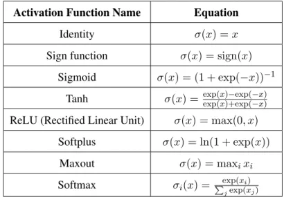
functions. These activation functions typically transform their input in an element-wise fashion, which is generally non-linear. In Table 2.4, we show a list of common activation functions. Note that all these functions operate on scalars, except for softmax and maxout, which take vectors as input. The softmax function is commonly used at the final layer, to convert the output into a probability distribution. This is particularly important for classification problems, where it is often desirable for a model to produce a probability distribution over the set of classes. In the classification context, using the softmax function to convert the output of the network into a probability distribution also allows the network to be trained using the cross-entropy (CE) loss function. On a single example x, with true labely, the cross-entropy loss penalizes a modelf which assigned probabilityfy(x)to
the correct label as follows:
Activation Function Name Equation
Identity σ(x) =x
Sign function σ(x) = sign(x) Si