Advanced Slicing of Sequential and Concurrent Programs

(1)

Advanced Slicing

of

Sequential and Concurrent

Programs

Jens Krinke

April 2003

(2)

(3)

Acknowledgments

First of all, I wish to thank my adviser Gregor Snelting for providing the sup-port, freedom and protection to do research without pressure. A big ‘sorry’ goes to him, to the second reviewer, Tim Teitelbaum, and to David Melski, be-cause this thesis has become longer than expected—thanks for reading it and the valuable comments.

Without the love and support of Uta von Holten, this work would not have been possible. She always believed in me, although this thesis took too long to finish. I thank my parents for enabling my career.

A big ‘thank you’ goes to my students who helped a lot by implement-ing parts of the presented techniques. First of all the former students at TU Braunschweig: Frank Ehrich, who implemented the user interface of the VAL-SOFT system (14.1.6) including the graphical visualization of program depen-dence graphs, slices and chops (9.1), Christian Bruns implemented the constant propagation (11.2.2), Torsten Königshagen implemented the call graph con-struction (11.2.1), Stefan Konst implemented the approximate dynamic slicing (14.1.8), and Carsten Schulz implemented the common subexpression elimina-tion (11.2.3). Students from Universität Passau were: Silvia Breu implemented the chop visualization (10.4), Daniel Gmach implemented the textual visual-ization of slices (9.2) and duplicated code (12.2.2), Alexander Wrobel mented the distance-limited slicing (10.1), and Thomas Zimmermann imple-mented some chopping algorithms (10.2).

Special thanks go to my colleagues in Passau, Torsten Robschink, Mirko Streckenbach, and Maximilian Störzer, who took over some of my teaching and administration duties while I finished this thesis. I also have to thank my former colleagues from Braunschweig, Bernd Fischer and Andreas Zeller for inspiration; they had the luck to finish their thesis earlier.

The Programming group at Universität Passau kindly provided the com-puting power that was needed to do the evaluations. Silvia Breu helped to improve the English of this thesis.

GrammaTech kindly provided the CodeSurfer slicing tool and Darren Atkin-son provided the Icaria slicer.

The VALSOFT project started as a cooperation with the Physikalisch-Tech-nische Bundesanstalt (PTB) and LINEAS GmbH in Braunschweig, funded by the former Bundesministerium für Bildung und Forschung (FKZ 01 IS 513

(4)

iv

C9). Later on, funding was provided by the Deutsche Forschungsgemeinschaft (FKZ Sn11/5-1 and Sn11/5-2).

(5)

Abstract

Program slicing is a technique to identify statements that may influence the computations in other statements. Despite the ongoing research of almost 25 years, program slicing still has problems that prevent a widespread use: Some-times, slices are too big to understand and too expensive and complicated to be computed for real-life programs. This thesis presents solutions to these prob-lems: It contains various approaches which help the user to understand a slice more easily by making it more focused on the user’s problem. All of these ap-proaches have been implemented in the VALSOFT system and thorough eval-uations of the proposed algorithms are presented.

The underlying data structures used for slicing are program dependence graphs. They can also be used for different purposes: A new approach to clone detection based on identifying similar subgraphs in program depen-dence graphs is presented; it is able to detect modified clones better than other tools.

In the theoretical part, this thesis presents a high-precision approach to slice concurrent procedural programs despite that optimal slicing is known to be undecidable. It is the first approach to slice concurrent programs that does not rely on inlining of called procedures.

(6)

(7)

List of Algorithms

2.1 Iterative computation of the MFP solution . . . 18

3.1 Slicing in PDGs . . . 34

4.1 Slicing Fine-Grained PDGs . . . 48

5.1 Slicing in tPDGs . . . 64

7.1 Summary Information Slicing (in SDGs) . . . 87

7.2 Computing Summary Edges . . . 89

7.3 Explicitly Context-Sensitive Slicing . . . 91

7.4 Folded Context-Sensitive Slicing . . . 94

8.1 Slicing Algorithm for tIPDGs,Sθ . . . 114

8.2 Improved Slicing Algorithm for tIPDGs . . . 115

10.1 Context-Insensitive Chopping . . . 132

10.2 Chopping with Summary Edges . . . 133

10.3 Mixed Context-Sensitivity Chopping . . . 134

10.4 Explicitly Context-Sensitive Chopping . . . 135

10.5 Merging Summary Edges . . . 136

10.6 Computation of Blocked Summary Edges . . . 145

11.1 Removing Redundant Nodes . . . 166

11.2 Removing Unrealizable Calls . . . 168

12.1 GenerateGk_n 1andG k n₂ . . . 180

(14)

(15)

List of Figures

1.1 A program dependence graph . . . 3

1.2 A procedure-less program . . . 3

1.3 A program with two procedures . . . 4

1.4 A program with two threads . . . 5

1.5 Another program with two threads . . . 6

2.1 Example program and its CFG . . . 14

2.2 A simple grammar with assignments as expressions . . . 19

2.3 Computation ofdef,refandacc . . . 19

2.4 Computation of may- and must-versions . . . 23

2.5 Computation of may- and must-versions ofgenandkill . . . . 24

2.6 The program dependence graph for figure 2.1 . . . 28

2.7 Example program and its CFG . . . 29

2.8 Modified CFG and its PDG . . . 30

3.1 Sliced example program and its PDG . . . 34

4.1 Excerpt of a fine-grained PDG . . . 42

4.2 Partial PDG for a use of structures . . . 43

4.3 Slices as computed by different slicers . . . 44

4.4 Partial PDG for a use of arrays . . . 45

4.5 Partial PDG for a use of pointers . . . 46

5.1 A threaded program . . . 52

5.2 A threaded CFG . . . 53

5.3 A tCFG prepared for control dependence . . . 58

5.4 A threaded PDG . . . 60

5.5 A program with nested threads . . . 61

5.6 The tPDG of Figure 5.5 . . . 62

5.7 Calculation ofSθ(4) . . . 66

5.8 A tCFG with communication dependence . . . 69

5.9 Control dependence for tCFG from figure 5.8 . . . 70

(16)

xvi LIST OF FIGURES

6.2 Interprocedural control flow graph . . . 77

6.3 ICFG with data dependence . . . 82

7.1 A simple example with a procedure . . . 86

7.2 Counter example for Agrawal’s ECS . . . 92

7.3 Details of the test-case programs . . . 96

7.4 Precision ofkLCS andkFCS (avg. size) . . . 97

7.5 Context-insensitive vs. context-sensitive slicing . . . 98

7.6 Precision ofkLCS (avg. size) . . . 99

7.7 Runtimes ofkLCS andkFCS (sec.) . . . 100

9.1 The graphical user interface . . . 122

9.2 A small code fragment with position intervals . . . 124

9.3 Intervals after transformation . . . 125

10.1 Evaluation of length-limited slicing . . . 128

10.2 Distance visualization of a slice . . . 130

10.3 Precision of MCC,kLCC andkFCC (in %) . . . 138

10.4 Context-insensitive vs. context-sensitive chopping . . . 139

10.5 Approximate vs. context-sensitive chopping . . . 140

10.6 Precision ofkFCC (avg. size) . . . 140

10.7 Runtimes ofkLCC andkFCC (in sec.) . . . 141

10.8 An example . . . 147

10.9 A chop for the example in figure 10.8 . . . 148

10.10 Another chop for the example in figure 10.8 . . . 149

10.11 Visualization of chops for all global variables . . . 152

10.12 GUI for the chop visualization . . . 153

11.1 Example for a PDG with cycles . . . 159

11.2 Size reduction and effect on slicing . . . 160

11.3 Size reduction and effect on chopping . . . 162

11.4 Size reduction and effect of context-insensitive folding . . . 162

11.5 Example for a SDG with redundant nodes . . . 163

11.6 Size reduction (amount of nodes and edges removed) . . . 167

11.7 A flawed C program . . . 170

11.8 PDG before common subexpression elimination . . . 172

11.9 PDG after common subexpression elimination . . . 173

12.1 Two similar pieces of code fromagrep . . . 176

12.2 Two simple graphs . . . 178

12.3 Visualization of similar code fragments . . . 182

12.4 Results forbison . . . 185

12.5 Running times ofbison . . . 187

12.6 Running times ofcompiler. . . 187

12.7 Results forcompiler. . . 188

(17)

LIST OF FIGURES xvii

12.9 Results for test casecook . . . 190

13.1 Simple fragment with program dependence graph . . . 194

13.2 Slice of the fragment . . . 194

13.3 Execution conditions . . . 195

13.4 Example with multiple definitions for variablex . . . 196

13.5 Example in SSA form . . . 197

13.6 Example for an interprocedural path condition . . . 205

13.7 Computation of PC2_NN(7, 10)for example 13.6 . . . 205

(18)

(19)

List of Tables

7.1 Precision . . . 102

11.1 Fine-grained vs. coarse-grained SDGs . . . 158

11.2 Time needed to fold cycles in SDGs . . . 160

11.3 Evaluation . . . 167

12.1 Some test cases . . . 183

12.2 Running times . . . 184

12.3 Sizes . . . 184

12.4 Participants . . . 189

(20)

(21)

Chapter 1

Introduction

Program slicing is a method for automatically decompos-ing programs by analyzdecompos-ing their data flow and control flow. Starting from a subset of a program’s behavior, slic-ing reduces that program to a minimal form which still produces that behavior. The reduced program, called a “slice”, is an independent program guaranteed to repre-sent faithfully the original program within the domain of the specified subset of behavior.

Mark Weiser [Wei84] Program slicing answers the question “Which statements may affect the computation at a different statement?”, something every programmer asks once in a while. After Weiser’s first publication on slicing in 1979, almost 25 years have passed and various approaches to compute slices have evolved. Usually, inventions in computer science are adopted widely after around 10 years. Why are slicing techniques not easily available yet? William Griswold gave a talk at PASTE 2001 [Gri01] on that topic: Making Slicing Practical: The Final Mile. He pointed out why slicing is still not widely used today. The two main problems are:

1. Available slicers are slow and imprecise. 2. Slicing ‘as-it-stands’ is inadequate to essential

software-engineering needs.

Not everybody agrees with his opinion. However, his first argument is based on the observation that research has generated fast and precise approaches but scaling the algorithms for real-world programs with million lines of code is still an issue. Precision of slicers for sequential imperative languages has reached a high level, but it is still a challenge for the analysis of concurrent programs— only lately is slicing done for languages with explicit concurrency like in Ada

(22)

2 Introduction

or Java. The second argument is still valid: Usually, slices are hard to under-stand. This is partly due to bad user interfaces, but is mainly related to the problem that slicing ‘dumps’ the results onto the user without any explana-tion.

This thesis will try to show how these problems and challenges can be tack-led. Therefore, the three main topics are:

1. Present ways to slice concurrent programs more precisely. 2. Help the user to understand a slice more easily

by making it more focused on the user’s problem. 3. Give indications of the problems and consequences

of slicing algorithms for future developers.

Furthermore, this thesis gives a self-contained introduction to program slic-ing. It does not try to give a complete survey because since Tip’s excellent sur-vey [Tip95]1the literature relevant to slicing has exploded: CiteSeer [LGB99] recently reported 257 citations of Weiser’s slicing article [Wei84] (and 95 for [Wei82]). This thesis only contains 187 references where at least 108 have been published after Tip’s survey.

1.1 Slicing

A slice extracts those statements from a program that potentially have an influ-ence on a specific statement of interest, which is the slicing criterion. Originally, slicing was defined by Weiser in 1979; he presented an approach to compute slices based on iterative data flow analysis [Wei79, Wei84]. The other main approach to slicing uses reachability analysis in program dependence graphs [FOW87]. Program dependence graphs mainly consist of nodes representing the statements of a program and control and data dependence edges:

• Control dependence between two statement nodes exists if one statement controls the execution of the other.

• Data dependence between two statement nodes exists if a definition of a variable at one statement might reach the usage of the same variable at another statement.

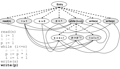
An example PDG is shown in figure 1.1 on the facing page, where control de-pendence is drawn in dashed lines and data dede-pendence in solid ones. How control and data dependence is computed will be presented in chapter 2.

(23)

1.1 Slicing 3

Entry

read(n) i := 1 s := 0 p := 1 while (i<=n) write(s) write(p)

i := i + 1 p := p * i s := s + i read(n) p := 1 i := 1 while (i<=n) p := p * i i := i + 1 write(s) write(p) s := s + i s := 0

Figure 1.1: A program dependence graph

1.1.1 Slicing Sequential Programs

Example 1.1 (Slicing without Procedures): Figure 1.2 shows a first example where a program without procedures shall be sliced. To compute the slice for the statementprint a, we just have to follow the shown dependences backwards. This example contains two data dependences and the slice includes the assign-ment toaand the read statement forb.

read a read b

a = 2*b print a read c

Figure 1.2: A procedure-less program

In all examples of this introduction, we will ignore control dependence and just focus on data dependence for simplicity of presentation. Also, we will always slice backwards from theprint astatement.

Slicing without procedures is trivial: Just find reachable nodes in the PDG [FOW87]. The underlying assumption is that all paths arerealizable. This means that a possible execution of the program exists for any path that executes the statements in the same order. Chapter 3 will discuss this in detail.

(24)

4 Introduction read a read b a = 2*b print a proc Q(): a = a+1 Q() Q() proc P(): . . . . . . . . . . . . . . . . Trace: P: read a P: read b Q: a = a+1 P: a = 2*b Q: a = a+1 P: print a

Figure 1.3: A program with two procedures

Example 1.2 (Slicing with Procedures): Now, the example is extended by adding procedures in figure 1.3. If we ignore the calling context and just do a traversal of the data dependences, we would add theread astatement into the slice for

print a. This is wrong because this statement has clearly no influence on the

print astatement. Theread astatement just has an influence on the first call of procedureQbutais redefined before the second call to procedureQthrough the assignmenta=2*bin procedureP.

Such an analysis is calledcontext-insensitivebecause the calling context is ig-nored. Paths are now considered realizable only if they obey the calling con-text. Thus, slicing iscontext-sensitive if only realizable paths are traversed. Context-sensitive slicing is solvable efficiently—one has to generate summary edges at call sites [HRB90]: Summary edges represent the transitive depen-dences of called procedures at call sites. How procedural programs are ana-lyzed will be discussed in chapter 6.

Within the implemented infrastructure to compute PDGs for ANSI C pro-grams, various slicing algorithms have been implemented and evaluated. One of the evaluations in chapter 7 will show that context-insensitive slicing is very imprecise in comparison with context-sensitive slicing. This shows that context-sensitive slicing is highly preferable because the loss of precision is not acceptable. A surprising result is that the simple context-insensitive slicing is slowerthan the more complex context-sensitive slicing. The reason is that the context-sensitive algorithm has to visit many fewer nodes during traversal due to its higher precision.

1.1.2 Slicing Concurrent Programs

Now, let’s move on to concurrent programs. In concurrent programs that share variables another type of dependence arises: interference. Interference occurs when a variable is defined in one thread and used in a concurrently executing thread.

(25)

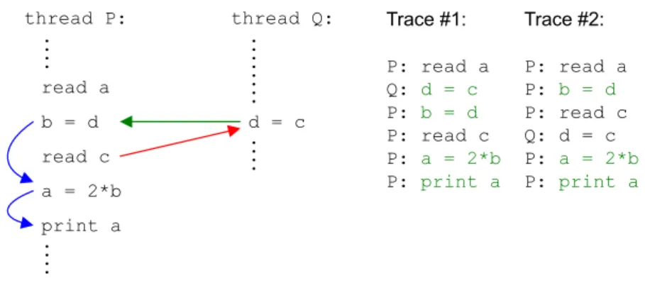
1.1 Slicing 5 read a b = d a = 2*b print a thread Q: thread P: . . . . . . . . . . . . . . . . d = c read c . . . . Trace #1: P: read a Q: d = c P: b = d P: read c P: a = 2*b P: print a Trace #2: P: read a P: b = d P: read c Q: d = c P: a = 2*b P: print a

Figure 1.4: A program with two threads

Example 1.3 (Slicing Concurrent Programs): In the example in figure 1.4 we have two threadsPand Qthat execute in parallel. In this example, there are two interference dependences: One is due to a definition and a usage of variabled, the other is due to accesses to variablec.

A simple traversal of interference during slicing will make the slice imprecise because interference may lead to unrealizable paths again. In the example in figure 1.4, a simple traversal will include theread cstatement into the slice. But there is no possible execution where theread cstatement has an influ-ence on the assignmentb=d. A matching execution would requiretime travel because the assignmentb=dis always executed before the read cstatement. A path through multiple threads is now realizable if it contains a valid execu-tion chronology. However, even when only realizable paths are considered, the slice will not be as precise as possible. The reason for this imprecision is that concurrently executing threads maykilldefinitions of other threads.

Example 1.4: In the example in figure 1.5 on the next page, theread a state-ment is reachable from theprint astatement via a realizable path. But there is no possible execution where thereadstatement has an influence on theprint

statement when assuming that statements are atomic. Either theread state-ment reaches the usage in thread Qbut is redefined afterwards through the assignmenta=2*bin threadP, or thereadstatement is immediately redefined by the assignmenta=2*bbefore it can reach the usage in threadQ.

Müller-Olm has shown that precise context-sensitive slicing of concurrent programs is undecidable in general [MOS01]. Therefore, we have to use con-servative approximations to analyze concurrent programs. A naive approx-imation would allow time travel, causing an unacceptable loss of precision. Also, we cannot use summary edges to be context-sensitive because summary edges wouldignorethe effects of parallel executing threads. Again, reverting to context-insensitive slicing would cause an unacceptable loss of precision.

To be able to provide precise slicing without summary edges, new slicing algorithms presented in chapter 7 have been developed based on capturing

(26)

6 Introduction read a read b a = 2*b print a thread Q: a = a+1 thread P: . . . . . . . . . . . . . . . . read c . . . . Trace #1: P: read a P: read b P: read c Q: a = a+1 P: a = 2*b P: print a Trace #2: P: read a P: read b P: read c P: a = 2*b Q: a = a+1 P: print a

Figure 1.5: Another program with two threads

the calling context throughcall strings [SP81]. Call strings can be seen as a representation of call stacks. They are used frequently for context-sensitive program analysis, e.g. pointer analysis. The call strings are propagated along the edges of the PDG: At edges that connect procedures the call string is used to check that a call always returns to the right call site. Thus, call strings are never propagated along unrealizable paths.

The basic idea for the high-precision approach to slice concurrent programs presented in chapter 8 is the adaption of the call string approach to concurrent programs. The context is now captured through one call string for each thread. The context is then a tuple of call strings which is propagated along the edges in PDGs.

A combined approach avoids combinatorial explosion of call strings: Sum-mary edges are used to compute the slice within threads. Additionally, call strings are only generated and propagated along interference edges if the slice crosses threads. With this approach many fewer contexts are propagated.

This only outlines the idea of the approach—this thesis will present in its first two parts the foundations and algorithms for slicing sequential and con-current programs in detail. Additionally, a major third part of this thesis will presents optimizations and advanced applications of slicing.

1.2 Applications of Slicing

Slicing has found its way into various applications. Nowadays it is probably mostly used in the area of software maintenance and reengineering. In the following some applications are mentioned to show the broadness but most will not be brought up in this thesis again.

(27)

1.2 Applications of Slicing 7

Debugging

Debugging was the first application of program slicing: Weiser [Wei82] real-ized that programmers mentally ignore statements that cannot have an influ-ence on a statement revealing a bug. Program slicing computes this abstraction and allows one to focus on potentially influencing statements. Dicing [LW87] can be used to focus even more, when additional statements with correct be-havior can be identified. Dynamic slicing can be used to focus on relevant statements for one specific execution revealing a bug [ADS93]. More work can be found in [FR01].

Testing

Program slicing can be used to divide a program into smaller programs spe-cific to a test case [Bin92]. This reduces the time needed for regression testing because only a subset of the test cases has to be repeated [Bin98].

In [HD95]robustness slices, which give approximate answer to the question whether a program is robust, are presented. Equivalent mutants can be de-tected by slicing [HHD99].

Other work to be mentioned can be found in [GHS92, BH93b]. Program Differencing and Integration

Programdifferencing is the problem of finding differences between two pro-grams (or between two versions of a program). Semantic differences can be found using program dependence graphs. Programintegrationis the problem of merging two program variants into a single program. With program de-pendence graphs it can be assured that differences between the variants have no conflicting influence on the shared program parts [HPR89, Hor90, HR91, HR92, RY89].

Software Maintenance

If a change has to be applied to a program, forward slicing can be used to iden-tify the potential impact of the change: The forward slice reveals the part of the program that is influenced by a criterion statement and therefore is affected by a modification to that statement. Decomposition slicing [GL91] uses variables instead of statements as criteria.

Function Extraction and Restructuring

Slicing can also be used forfunction extraction[LV93, LV97]: Extractable func-tions are identified by slices specified by a set of input variables, a set of output variables and a final statement. Function restructuringseparates a single func-tion into independent ones; such independent parts can be identified by slicing [LD98, LD99].

(28)

8 Introduction

Cohesion Measurement

Ott et al [OT89, Ott92, OT93, BO94, OB98] use slicing to measure functional co-hesion. They define data slices which are a combination of forward and back-ward slices. Such slices are computed for output parameters of functions and the amount of overlapping indicates weak or strong functional cohesion.

Other Applications

Slicing is used in model construction to slice away irrelevant code, transition system models are only build for the reduced code [HDZ00]. Slicing is also used to decompose tasks in real-time systems [GH97]. It has even been used for debugging and testing spreadsheets [RRB99] or type checking programs [DT97, TD01].

1.3 Overview

This thesis is structured into three parts: First, intraprocedural analysis, sec-ond, interprocedural analysis and slicing of sequential and concurrent pro-grams, and last, another main part: applications of dependence graphs and slicing.

The first part starts with an introduction to data flow analysis in the next chapter. It is followed by an introduction to slicing based on Weiser’s original definition and on program dependence graphs. Chapter 4 presentsfine-grained program dependence graphs and how ANSI C programs can be represented with them. The last chapter of the first part presents an approach to slicing concurrent programs (without procedures).

The second part is structured similarly to the first one: It starts with an in-troduction to interprocedural data flow analysis. Interprocedural slicing based on program dependence graphs is presented next in chapter 7, which also con-tains an evaluation of various algorithms. The last chapter of part two de-scribes the new approach to slicing concurrent procedural programs.

The third and main part contains applications. The starting chapter presents two approaches to visualize dependence graphs both graphically and textually. Chapter 10 contains various solutions to the problem that a traditional slice is not focused and usually too large. That chapter also presents and evaluates various chopping algorithms. Chapter 11 shows some approaches to reducing the size of dependence graphs and to increasing their precision. Clone detec-tion based on program dependence graphs is addressed in chapter 12. Path conditions answer the question why a specific statement is in a slice; they are presented in chapter 13. Chapter 14 describes the VALSOFT system in which most of the presented work has been implemented. The last chapter completes this thesis with conclusions.

(29)

1.4 Accomplishments 9

1.4 Accomplishments

This thesis is self-contained as much as possible and therefore contains presen-tations of other authors’ work. Besides a thorough presentation of slicing, the accomplishments of this thesis are:

• A fine-grained program dependence graph (chapter 4), which is able to represent ANSI C programs including non-deterministic execution order. It is a self-contained intermediate representation and the base of clone detection and path condition computation.

• A high-precision approach to slicing concurrent procedure-less programs (chapter 5). A preliminary version has been published as [Kri98].

• A new approach to slicing concurrent procedural programs (chapter 8). This context-sensitive approach reaches a high precision, despite that precise or optimal slicing is undecidable. This is the first approach that does not need inlining and is able to slice concurrent recursive programs.

• Some variations of slicing and chopping algorithms within interprocedu-ral program dependence graphs and a thorough evaluation of these algo-rithms (sections 7.3, 7.4, 10.2). Most of this has already been published in [Kri02].

• Fundamental ideas to visualizing dependence graphs (chapter 9), real-ized in Ehrich’s master’s thesis [Ehr96].

• Some methods to make the results of slicing more focused (sections 10.1 and 10.3) or more abstract (section 10.4).

• Techniques to reduce the size of program dependence graphs without worsening the precision of slicing (section 11.1).

• An approach to clone detection based on program dependence graphs (chapter 12). This approach has a higher detection rate for modified clones than other approaches, because it identifies similar semantics in-stead of similar texts. After publication in [Kri01], the benefits and draw-backs of this approach have been evaluated in a clone detection contest.

• Methods to generate path conditions for complex data structures, proce-dures and concurrent programs (sections 13.2, 13.4 and 13.5). The general approach of path conditions was introduced by Snelting [Sne96] and de-veloped further by Robschink [Rob, RS02, SRK03].

• The design of the VALSOFT system and implementation of the data flow analysis, dependence graph construction and various slicing and chop-ping algorithms within it (chapter 14).

(30)

(31)

Part I

(32)

(33)

Chapter 2

Intraprocedural Data Flow

Analysis

The following introduction to intraprocedural data flow analysis is based on the problem ofReaching Definitions. A definition is a statement that assigns some value to a variable. Usually, reaching definitions are not defined by the statements in a program, but in terms of the control flow graph, which repre-sents the flow of control between the statements of a program. A definition is said to reach a given statement if there is a path from the definition to the given statement without another definition of the same variable. Such a second def-inition wouldkillthe first—which will no longer reach the given statement on thatpath (it may still reach the given statement on a different path).

2.1 Control Flow Analysis

To analyze a program, thecontrol flow—the possible execution sequences of the statements—must be understood first. This is obvious with only well-structured constructs. However, as soon as constructs like goto statements are involved that may lead to unstructured programs, the identification of possi-ble control flow is non-trivial. For this reason, a graph-based representation is usually used. This so-calledflow graphis built out of the nodes representing the statements and the edges representing the flow of control in between. In con-trast to analysis for optimization purposes, we don’t merge statements tobasic blocks—instead, our goal is that any node represents at most one side effect.

Acontrol flow graph(CFG) is a directed attributed graphG= (N,E,ns,ne,ν) with node setNand edge setE. The statements and predicates are represented by nodesn ∈ N and the control flow between statements is represented by control flow edges(n,m)∈E, written asn*m.Econtains control flow edgee, iff the statement represented by nodetarget(e)may immediately be executed after the statement represented bysource(e), i.e. no other statement is executed

(34)

14 Intraprocedural Data Flow Analysis 1 sum = 0 2 mul = 1 3 a = 1 4 b = read() 5 while (a <= b) { 6 sum = sum + a 7 mul = mul * a 8 a = a + 1 9 } 10 write(sum) 11 write(mul)

Figure 2.1: Example program and its CFG

in between. Two special nodesns ∈ N and ne ∈ N are distinguished, the STARTnodensand the EXITnodene, which represent beginning and end of the program. Nodensdoes not have predecessors and nodenedoes not have successors. The functionν : E → {true,false,}is a mapping of the edges to their attributes: If the statement represented by source(e) has an out-degree

>1, it contains a predicate controlling which statement is executed afterwards and the outgoing edges are attributed withtrueorfalse—the outcome of the predicate. Other edges are marked with, which means not attributed. Example 2.1: Figure 2.1 shows a small program and its control flow graph. The nodes are numbered with the corresponding line number of the represented statement.

The variables that are referenced at node1nare denoted byref(n), the variables that are defined (or assigned) atnare denoted bydef(n). Both functions can be bound more formally to the nodes by extending the definition of the control flow graph toG = (N,E,ns,ne,µ,ν), where µis a function mapping nodes to their attributes. It is defined asµ(n) = (def(n),ref(n))orµdef(n) = def(n),

µref(n) =ref(n).

Most interesting problems are questions as to whether something (some information or property) at a nodenreachesa different nodem. Part of such a question is whether nodemisreachable fromnat all. Formally, a node n

isreachable(m *? _n_{) from another node}_m_{, if there is a path}_h_m_{, . . . ,}_n_i_in_G_,

i. e. “*?_{” is the transitive, reflexive closure of “}_*_{”. Normally it is assumed} 1_{In the rest of this work we will use “node” and “statement” interchangeable, as they are}

(35)

2.2 Data Flow Analysis 15

that for any path in the CFG a corresponding execution of the program exists, such that all statements are executed in the same order as the nodes of the path. Of course, this is only a conservative approximation, as paths might exist that are actuallyunrealizable. However, in general this is undecidable and therefore all paths are assumedrealizable.

If we pick some statements out of the node sequence of a path they are a witnessof a possible path:

Definition 2.1 (Witness)

A sequence hn1, . . . ,nki of nodes is called a witness, iff ni *? ni+1 for all 16i < k.

This means that a sequence of nodes is a witness, if all nodes are part of a path through the CFG in the same order as in the sequence. Of course, every path is a witness of itself, but a sequence can be a witness of multiple different paths.

Normally, the nodes of the flow-graph can be constructed in a syntax-directed way during parsing. Most of the edges can be constructed that way, too. Edges for goto statements etc. can be back-patched.

2.2 Data Flow Analysis

The purpose of data flow analysis is to compute the behavior of the analyzed program in respect to the generated data, usually used for program optimiza-tions, i.e. to check the circumstances for the application of optimizations. The easiest and most widespread solutions are analyses that iterate over the con-trol flow graph (callediterative data flow analysis). Another approach omits the control flow graph and does the analysis directly on top of the (abstract) syn-tax tree (calledsyntax-directed data flow analysis). Both approaches are presented next.

2.2.1 Iterative Data Flow Analysis

The discussion of the reaching definitions example is resumed by formalizing the problem:

Definition 2.2 (Reaching Definitions)

For any noden∈Nin flow-graphG, letdef(n)be the set of variables defined atn. A definition of variablevat a noden(v∈def(n))reachesa (not necessarily different) noden0, if a pathP=hn1, . . . ,nkiinGexists, such that

1. k >1

2. n₁=n∧nk=n0 3. ∀1< i < k:v /∈def(ni)

(36)

16 Intraprocedural Data Flow Analysis

The computation of reaching definitions can be described within a data flow analysis framework. Therefore, the local abstract semantics are described with a transfer function over the set of definitionsxthat reach a noden:

[[n]](x) = x−kill(n)∪gen(n)

This equation means that definitions reaching the entry of a nodenwhich are not killed byn, reach the exit ofntogether with definitions generated byn. Definitions can be represented in multiple ways. One possibility is to represent them by node-variable pairs(n,v)containing the variablevthat is defined at

n:

gen(n) = {(n,v)|v∈def(n)}

kill(n) = {(n0,v)|v∈def(n)∧v∈def(n0)}

Such representations can be simplified by enumerating all occurring defini-tions: the setD contains all definitions of a program, the setsDv contain all definitions for a specific variablevand the setsDncontain all definitions at a noden. Then the equations are

gen(n) = Dn

kill(n) = [ v∈def(n)

Dv

which are constant functions.

The next step is to define the abstract semantics over a pathp=hn₁, . . . ,nki, with the identity function[[]]_id(x) =x:

[[p]] =

[[]]_id p=hi

[[hn₂, . . . ,nki]]◦[[n1]] otherwise

A definition reaches a noden, if a path from theSTARTnodenstonexists, on which the definition is not killed according to definition 2.2 on the page before. At theSTARTnode, no definition is available (an empty set of definitions). If there exists more than one path, the reaching definitions of all paths are merged (by union in this case):

RD_MOP(n) = [ p=hs,...,ni

[[p]](∅)

This is an instance of ameet-over-all-paths (MOP)solution. In presence of loops there are infinite paths, which make the computation of the MOP solution im-possible. Therefore, only theminimal-fixed-point (MFP)solution2is computed:

RD_MFP(n) =

∅ n=s

[[n]](S

m*nRDMFP(m))

(37)

Because of the properties of the transfer functions and the data flow sets, the MFP and the MOP solution coincide: The data flow sets form a (complete) semi-lattice and the transfer functions form a distributive function space: Definition 2.3 (Lattice)

AlatticeL= (C,u,t)consists of a set of valuesC, ameetoperationuand ajoin operationt, such that

1. ∀x∈C:xtx=xandxux=x(idempotency)

2. ∀x,y∈C:xty=ytx∧xuy=yux(commutativity)

3. ∀x,y,z∈C: (xty)tz=xt(ytz)∧(xuy)uz= xu(yuz) (associa-tivity)

4. ∀x,y∈C:xt(xuy) =xandxu(xty) =x(absorption)

With only one operatorL= (C,t)is asemi-lattice. A (semi-) lattice induces a partial ordervon the elements ofC.

Lattices are used to represent thedata flow facts, in the example of reaching definitions the sets of definitions. Most data flow facts are sets, where the lattice is the powerset. This can be represented as bit-vectors: if the set of data flow facts isD, thanC=2D.

Definition 2.4 (Monotone Function Space)

A set of functionsFdefined on semi-latticeL = (C,t)is amonotone function space, if

1. ∀f∈F:∀x,y∈C:xvy⇒f(x)vf(y)(monotonicity) 2. ∃f_id ∈F:∀x∈C:f_id(x) =x(identity function) 3. ∀f,g∈F: f◦g∈F ∧∀x∈C:f◦g(x) =f(g(x))

(closed under composition)

Definition 2.5 (Data Flow Analysis Framework)

Amonotone data flow analysis frameworkA= (L,F,t)consists of

1. the (complete) semi-latticeL= (C,t)with meettfor the data flow facts, and

2. the monotone function spaceFdefined onL.

A monotone data flow analysis framework is a distributive data flow analysis framework, if∀f∈F:∀x,y∈C:f(xty) =f(x)tf(y).

The iterative algorithm 2.1 on the following page of a monotone data flow analysis framework computes the MFP solution; the monotonicity guarantees termination and the existence of a fix-point. The MFP solution is a correct albeit not necessarily precise solution of the data flow problem. It coincides

(38)

Algorithm 2.1Iterative computation of the MFP solution Input:The control flow graphG= (N,E,ns,ne)

The function spaceFof transfer function[[n]]

The semi-latticeL= (C,t)of the data flow information An initial valuei∈C

Output:The mappinginfrom nodes to its data flow information

foreachn∈Ndo

in[n] =⊥

in[ns] =i

Initialize the worklist:

W={n|ns*n∈E}

whileW6=∅,worklist is not emptydo

W=W/{n},remove one element from worklist

v=F m*n∈E[[m]](in[m]) ifv6=in[n]then in[n] =v W=W∪{m|n*m∈E} returnin

with the correct and precise MOP solution if it is based on a distributive data flow analysis framework.

The equations of the reaching definitions fit in a distributive data flow anal-ysis framework:

• The semi-latticeLis the powerset of the setDof all definitions in a pro-gram (C=2D), with meet operatort=∪.

• The function spaceFis the set of all transfer functions[[n]]including the identity[[]]_id.

It can be proved that the function space is a distributive function space and therefore the algorithm for the MFP solution computes the correct and precise MOP solution.

2.2.2 Computation of

def

and

ref

for ANSI C

Up to now, the existence ofdefandref has been assumed. However, the com-putation ofdef andref are non-trivial in presence of complex data structures. This thesis focuses on the analysis of ANSI C [Int90], which makes the analysis of expressions a complex task when the original program is not transformed into a simpler intermediate representation first. The execution order in expres-sions is (mostly) undefined in ANSI C and expresexpres-sions cannot be represented in a control flow graph structure. Therefore the expressions’ subtrees are copied from the abstract syntax tree into the nodes of the control flow graph. The rest

(39)

E → s E → c E → E₁+E₂ E → E₁=E₂

Figure 2.2: A simple grammar with assignments as expressions

E₁→s₂ : (d1,r1,a₁) = (∅,∅,{(n,vs)})

E₁→c : (d₁,r₁,a₁) = (∅,∅,∅)

E₁→E₂+E₃ : (d1,r1,a₁) = (d₂∪d3,r₂∪r₃∪a₂∪a3,∅)

E₁→E₂=E₃ : (d₁,r₁,a₁) = (d₂∪d₃∪a₂,r₂∪r₃∪a₃,∅)

Figure 2.3: Computation ofdef,refandacc

of this section shows howdef andref can be computed in a syntax-directed way via the copied expression subtrees.

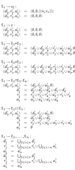
Figure 2.2 shows a grammar for simple expressions to start with. As in C, expressions can be used asl-orr-values, which means as targets of assignments (to theleft) or as expressions to be evaluated (to therightof assignments). This has to be distinguished if a variables(a symbol) is accessed in an expression. Therefore, a third setaccis used in addition todef andref which captures the accessed variables. For productionE→sthe access ofsif represented by(n,v): variablevis accessed at the nodenin the abstract syntax tree. Because it is not clear if the access tovis a use or a definition, onlyacc is set to{(n,v)}, while

refanddef are empty. An access to a constant (E →c) generates no access to a variable. An operation on expressions like in productionE →E₁+E₂causes the evaluation ofE₁andE₂and any variable that is accessed inE₁orE₂must now be put intoref. A definition through an assignment E → E₁=E₂causes the variables accessed inE₁to be defined and put intodef, while the variables accessed inE₂are evaluated and put intoref. This behavior is represented as equations in figure 2.3, where(d,r,a)is used as a shorthand for(def,ref,acc).

Arrays

Now, a productionE →a[E₁]is added to allow array usage in the program. In general it is undecidable if two array usagesa[E₁]and a[E₂]access the same array element. Therefore all elements of an array are accesses to the array variable. An assignment to an array element only kills one element and leaves the other untouched. There are two approaches to modeling this:

(40)

1. Any assignment to an array element is assumed to be anon-killing assign-ment, i.e. a new definition is created, but none eliminated. The equations are extended with

E₁→E₂[E₃] : (d1,r1,a₁) = (d₂∪d3,r₂∪r₃∪a3,a₂)

and also the previous definition ofkill(n)must be changed that no array variable is killed:

kill(n) = {(n0,v)|v∈def(n)∧v∈def(n0)∧vis not an array} 2. Any assignment to an array element is assumed to be akilling

modifica-tion, i.e. the array is used before killed (the array is modified). Then the equations are extended with

E₁→E₂[E₃] : (d1,r1,a₁) = (d₂∪d3,r₂∪r₃∪a₃∪a2,a₂) and the definition ofkill(n)stays unchanged.

Both approaches are conservative approximations and must be chosen depen-dent on the intended application. Due to other reasons which will be explained later, the killing modification is the preferred way in this work.

Structures and Unions

ANSI C allows aggregation of types to complex data types, called structures and unions. A variable of structure or union type contains fields that can be accessed without accessing the other fields. To handle structures and unions scalar replacementis used. Any access to a variable (or a field of a variable) is replaced by accesses to the contained fields as scalar variables. Because fields can be structures or unions themselves, this is done recursively. Let SR(v) re-turn the set of variables generated by scalar replacement for a variablev. Then the equations are extended and modified with:

E₁→E₂.f : (d₁,r₁,a₁) = (d₂,r₂,{(n,vi.f)|(n,vi)∈a2}) The scalar replacement is done in thekill(n)andgen(n)functions:

gen(n) = {(n,v)|v0∈def(n)∧v∈SR(v)}

kill(n) = {(n0,v)|v0∈def(n)∧v0∈def(n0)∧v∈SR(v0)}

Unions cause a slight problem because the fields of a union share the same space: an access to a field may access some other fields of the union, too. Again, this is handled through the scalar replacement: Let UR(v) return the set of variables which share a union with variablev.

gen(n) = {(n,v)|v0∈def(n)∧v∈SR(v0)∪UR(v0)}

kill(n) = {(n0,v)|v0∈def(n)∧v0∈def(n0)∧v∈SR(v0)}

Because it is compiler dependent which other fields of a union share the space with an accessed field, a definition must not kill other fields of the union.

(41)

Pointer Usage

A real problem is the presence of pointers: They cannot be tackled by a simple solution like scalar replacement. A special data flow analysis is needed which also handles the combination with structures, unions and arrays. Pointer anal-ysis is too complex to be discussed here and we assume a function PT(v,n) that returns—for an access to a variablev—the set of variablesvcan point to atn. Again, this function is integrated into thekill(n)andgen(n)functions us-ing the scalar replacement. An extensive amount of literature exists for pointer and alias analysis and among hundreds of works, [HP00, Hin01] can be used for an introduction. For the analysis system which will be discussed later, a flow-insensitive but context-sensitive alias analysis of Burke et al [BCCH95] has been implemented.

The equations are extended to obey pointer usage:

E₁→&E₂ : (d1,r1,a₁) = (d1,r1,{(n, &v)|(n,v)∈a₂} E₁→*E₂ : (d1,r1,a₁) = (d1,r1,{(n,∗v)|(n,v)∈a₂} E₁→E₂->f : (d1,r1,a₁) = (d1,r1,{(n,∗v.f)|(n,v)∈a₂}

Other Forms of Assignments

ANSI C knows a series of special forms of assignments that are trivial to ana-lyze:

E₁→E₂+=E₃ : (d₁,r₁,a₁) = (d₂∪d₃∪a₂,r₂∪r₃∪a₃,a₂)

E₁→++E₂ : (d1,r1,a₁) = (d₂∪a2,r₂∪a2,a₂)

where+=stands for any modifying assignment and++stands for any pre- or post-modifying operator.

2.2.3 Control Flow in Expressions

For some expressions, ANSI C defines an execution order. It even allows some expressions to be evaluated or not. Examples for such expressions are:

Comma operator. Expressions separated by the comma operator are evalu-ated in left-to-right order and the rightmost expression is used as result. All expressions to the left of a comma are evaluated (r-value expressions) and the last expression can be used as ar-value or even as anl-value, e.g.

(a,b,c).for(x,y)=(a,b)is possible.

Question-mark operator. The question-mark operator is like an ‘if’ for expres-sions. Depending on the outcome of the predicate to the left of the ques-tion operator?, one of the two expressions to the right is used asr- or l-value, e.g.a=x?y:zor evenx?y:z=a.

(42)

Shortcut operator. Predicates using logical shortcut operators||or&&allow to skip the evaluation of the expression to the right of the operator if the result of the complete expression is clear after evaluating the expression to the left. For example inp || qthe expressionqmust not be evaluated ifphas been evaluated totrue.

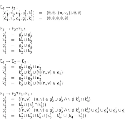
For compiling purposes, such expressions are normally transformed to state-ments first, so that a control flow graph can be used and all expressions are free of control flow. Again, if transformations are not allowed, these expres-sions need special attention. First of all, definitions (and uses) have to be dis-tinguished betweenmusthappen and mayhappen: a definition to the left of a shortcut operator must happen, if the complete expression is evaluated, but a definition to the right may or may not happen. Second, all equations must be extended to computedef,ref andaccin and must-versions. The may-versions are notated asd?,r?,a?and the must-versions asd!,r!,a!. Some of the equations are shown in figure 2.4 on the next page.

Because these three classes of operations define control flow inside expres-sions, thekillingof uses and definitions must be obeyed. The presented equa-tions ignore killing so far. Instead of changingdef,ref andacc, the equations are extended to already computekillandgen. For presentation purposes, only some extended equations are shown in figure 2.5 on page 24 and aliasing and scalar replacement is ignored.

2.2.4 Syntax-directed Data Flow Analysis

A different approach to the problem of reaching definitions is to ignore the control flow graph and to solve it based on the abstract syntax tree. The key insight is that in well-structured programs the control flow is obvious. The following equations show how the transfer functions are combined:

[[if E then S₁ else S₂]] = ([[S₁]]∪[[S₂]])[[E]] [[S₁]];[[S₂]] = [[S₂]][[S₁]]

[[]] = [[]]_id

Under the condition that[[S]][[S]] = [[S]]holds (for reaching definitions), the fol-lowing equation is valid:

[[while E do S₁]] = [[E]]∪([[E]][[S₁]][[E]])

This might raise the impression that a syntax-directed approach is easier to implement than an iterative framework. However, this is a wrong impression— looking at the syntax-directed computation ofgenandkillin the previous sec-tions, you get a glimpse of an implementation’s complexity. The problem is not the theoretical complexity, but the sheer amount of implementation work. De-spite that, the implementation of the analysis tool presented in the next chap-ters includes a traditional as well as a syntax-directed computation of reaching definitions for evaluation and debugging purposes.

(43)

2.2 Data Flow Analysis 23 E₁→s₂: (d₁!,r!₁,a!₁) = (∅,∅,{(n,vs)}) (d₁?,r?₁,a?₁) = (∅,∅,∅) E₁→c: (d₁!,r!₁,a!₁) = (∅,∅,∅) (d₁?,r?₁,a?₁) = (∅,∅,∅) E₁→E₂+E₃: (d₁!,r!₁,a!₁) = (d!₂∪d!₃,r!₂∪r!₃∪a!₂∪a!₃,∅) (d₁?,r?₁,a?₁) = (d?₂∪d?₃,r?₂∪r?₃∪a?₂∪a?₃,∅) E₁→E₂=E₃: (d₁!,r!₁,a!₁) = (d!₂∪d!₃∪a!₂,r!₂∪r!₃∪a!₃,∅) (d₁?,r?₁,a?₁) = (d?₂∪d?₃∪a?₂,r?₂∪r?₃∪a?₃,∅) E₁→E₂?E₃:E₄: (d₁!,r!₁,a!₁) = (d!₂,r!₂∪a!₂,∅) d?₁ = d?₂∪d?₃∪d?₄∪d₃! ∪d!₄ r₁? = r?₂∪r?₃∪r₄?∪a?₂∪r₃! ∪r!₄ a?₁ = a?₃∪a?₄∪a₃! ∪a!₄ E₁→E₂||E₃: (d₁!,r!₁,a!₁) = (d!₂,r!₂∪a!₂,∅) d?₁ = d?₂∪d?₃∪d!₃ r?₁ = r?₂∪r?₃∪a?₂∪a₃?∪r!₃∪a₃! a?₁ = ∅ E₁→E₂,. . .,En: d!₁ = S 26i6nd!i r!₁ = S 26i6nr!i∪ S 26i<na!i a!₁ = a_n! d?₁ = S 26i6nd?i r?₁ = S 26i6nr?i∪ S 26i<na?i a?₁ = a_n?

(44)

24 Intraprocedural Data Flow Analysis E₁→s₂: (d!₁,r!₁,a!₁,g!₁,k!₁) = (∅,∅,{(n,vs)},∅,∅) (d?₁,r?₁,a?₁,g?₁,k?₁) = (∅,∅,∅,∅,∅) E₁→E₂+E₃: g₁! = g₂! ∪g!₃ k₁! = k!₂∪k!₃ g₁? = g₂?∪g?₃ k₁? = k?₂∪k?₃ E₁→E₂=E₃: g₁! = g₂! ∪g!₃∪a₂! k₁! = k!₂∪k!₃∪{v|(n,v)∈a!₂} g₁? = g₂?∪g?₃∪a₂? k₁? = k?₂∪k?₃∪{v|(n,v)∈a?₂} E₁→E₂?E₃:E₄: g₁! = {(n,v)|(n,v)∈g!₂∪a!₂∧v /∈k₃! ∩k!₄} k₁! = k!₂∪(k!₃∩k!₄)) g₁? = {(n,v)|(n,v)∈g?₂∪a?₂∧v /∈k₃! ∩k!₄}∪g₃?∪g?₄∪g!₃∪g!₄ k₁? = k?₂∪k?₃∪k?₄∪(k!₃−k₄!)∪(k₄! −k!₃))

(45)

2.3 The Program Dependence Graph 25

The syntax-directed approach is even possible with well-structured jumps like break, continue or return statements. This is based on a simple trick: every statement (which may contain other statements) is assumed to be left through one of four possible exits:

1. The statement is entered, computation proceeds and it is left normally; no jump is encountered.

2. The statement is entered and left by a return statement (after some com-putation).

3. The statement is left by a break statement, or 4. by a continue statement.

Now, for every statement four matching transfer functions are defined describ-ing the data flow on each of the four possible executions.

2.3 The Program Dependence Graph

Aprogram dependence graph[FOW87] is a transformation of a CFG, where the control flow edges have been removed and two other kinds of edges have been inserted:control dependenceanddata dependenceedges. These edges repre-sent the effects of control flow and reaching definitions more directly: control dependence exists, if one statement is controlling the execution of a different statement. Data dependence exists, if a definition at a node reaches a different node and is used there.

2.3.1 Control Dependence

Nodemis called apost-dominatorof Noden, if any path fromnto theEXITnode

nemust go throughm. A nodenis called apre-dominatorofmif any path from theSTARTnodenstommust go throughn. In typical programs, statements in loop bodies are pre-dominated by the loop entry and post-dominated by the loop exit.

Definition 2.6 (Control Dependence)

A nodemis called(direct) control dependenton noden, if 1. there exists a pathpfromntomin the CFG (n*? _m_),

2. mis a post-dominator for every node inpexceptn, and 3. mis not a post-dominator forn.

This basically means that at nodenat least two outgoing edges exist: all paths to theEXITnode along one edge pass throughmand all paths along the other edge don’t.

(46)

Depending on the definition whether a node post- or pre-dominates itself, a node can be control dependent on itself. Some authors do not allow this, some do. If a node post-dominates itself, the predicate of a while loop is control dependent on itself. On the other hand, if a node never post-dominates itself, the control dependences of while loops and if-statements are identical.

There are two ways to compute control dependence: the traditional and the syntax-directed approach, which will both be presented next.

Syntax-directed Computation of Control Dependence

Within well-structured programs that just containif-statements and loops with-out jump statements likegoto,break,continueorreturn, the control depen-dence can easily be computed during traversal of the abstract syntax tree:

• Every statement is directly control dependent on its enclosingif- or loop-statement predicate.

• If nodes post-dominate themselves, every loop-statement predicate is control dependent on itself.

An important observation is that when nodes never post-dominate them-selves, the control dependence subgraph of a well-structured program is a tree. Traditional Computation of Control Dependence

The traditional approach to compute control dependence is to first compute the post-dominator tree with the fast Lengauer-Tarjan algorithm [LT79]. The second step is to traverse all control flow edges: For everym*nthe ances-tors ofnin the post-dominator tree are traversed backwards to the parent of

m, marking all visited nodes as control dependent on m(see [FOW87] for a detailed description).

2.3.2 Data Dependence

Two nodes are data dependent on each other, if a definition at one node might be used at the other node:

Definition 2.7 (Data Dependence)

A nodemis calleddata dependenton noden, if

1. there is a pathpfromntomin the CFG (n*? _m_),

2. there is a variablev, withv∈def(n)andv∈ref(m), and 3. for all nodesk6=nof pathp,v /∈def(k)holds.

This is very much similar to the problem of reaching definitions: if a defini-tion of a variablevat nodenis a reaching definition atmandmuses variable

v, thenmis data dependent onn. Thus, the computation of data dependence is straightforward: compute the reaching definitions first and then check every node if it uses a variable of a reaching definition.

(47)

2.3 The Program Dependence Graph 27

2.3.3 Multiple Side Effects

Up to now, the possibility of multiple side effects in expressions has been ig-nored. Because assignments are expressions, an expression may contain multi-ple assignments. In ANSI C it is common to make use of multimulti-ple assignments: pre- and post-modifying operators are very comfortable and typically used as inx = a[i++]. But what happens inside a single expression if a variable has a side effect and is accessed a second time? The ANSI C standard [Int90] allows an undefined behavior under such circumstances. This is adequate for com-pilers, but not for reverse engineering, program understanding or debugging purposes. There are two ways to deal with this:

1. Follow the ANSI C standard and ignore data dependence inside expres-sions. This might be awkward for users especially in conjunction with procedure calls (an example will be given in section 4.1).

2. Allow data dependence inside expressions. However, these dependences cannot be ‘back-patched’ while computing kill and gen: an expression likex = x+1contains a use and a definition ofx, but has no inside data dependence. Therefore the equations for(d,r,a,g,k)must be extended to compute the generated data dependences.

The implemented analysis system uses the second approach. However, the extensions to the equations will provide no new insights and thus are not pre-sented here.

2.3.4 From Dependences to Dependence Graphs

Once the control and data dependence have been computed, it is a simple task to build a dependence graph: Theprogram dependence graph (PDG)consists of the nodes of the CFG, control dependence edgesn*cd mfor nodesmwhich are control dependent on nodesn, and data dependence edgesndd*mfor nodes

mwhich are data dependent on nodesn.

Example 2.2: Figure 2.6 on the next page shows the PDG for the example in figure 2.1 on page 14. The nodes are exactly those of the corresponding control flow graph, except for the absentEXITnode.

Without modifications, the control dependence subgraphs have no single root because the top most statements will not be control dependent on any-thing. On the other hand, it is desirable that there exists a single root, which should be theSTARTnode. This is usually achieved by inserting an irrelevant control flow edge from theSTARTto theEXITnode. The effect is that no other node than theEXITnode post-dominates theSTARTnode and theSTARTnode will be the root in the control dependence subgraph. Normally, theEXITnode will be omitted from the program dependence graph, as it has no in- or outgoing dependence edges. The irrelevant edge is ignored during data flow analysis.

(48)

Figure 2.6: The program dependence graph for figure 2.1

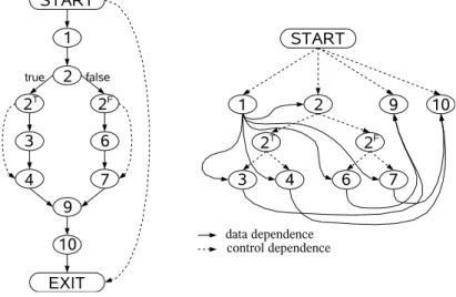
This special handling of theSTARTnode can be seen as the introduction of aregionnode that joins nodes of a region. In [FOW87] such nodes are inserted at several places. It is observed that control dependence is nonintuitive, as a predicate node has more than one outgoing control dependence edge marked withtrueand mixed with more than one marked with false. The purpose of region nodes is to summarize the set of outgoing control dependence edges with the same attribute and group together all nodes with incoming control dependence edges coming from the same node with the same attribute. The result is that predicate nodes have only two successors like in the control flow graph. An algorithmic solution which inserts such region nodes is given in [FOW87]. Instead, it is now shown how such region nodes can be inserted by a modified construction of the control flow graph.

Remember the insertion of an irrelevant edge to makeSTARTa region node. The insertion of irrelevant edges can also be used for insertion of other region nodes. In well structured programs, the regions which should be summarized can be identified clearly as single-entry-single-exit blocks. Between the pred-icate node and the entry of such a block a control flow edge attributed with

trueorfalseexists. The first step is to insert a region node before the entry node, an unattributed control flow edge from the region to the entry node and redirect the attributed control flow edge to the region node instead. The region node will use the identity transfer function[[]]_idand therefore this modification has no influence on the results of the data flow analysis. The second modifica-tion is to insert an irrelevant edge from the region node to the successor of the block’s exit node. Because the program is well structured, the node has only one successor.

Example 2.3: Figure 2.7 on the next page shows a small program and its (tra-ditional) CFG. First, the modifications will insert an irrelevant edge between STARTandEXIT. Next, two new region nodes are inserted for the two single-entry-single-exit regions consisting of nodes 3/4 and 6/7. They are also con-nected to the predicate node and the last node of their region (nodes 4 resp. 7). The resulting CFG is shown in Figure 2.8 on page 30, together with the

Advanced Slicing of Sequential and Concurrent Programs