Optimized Multichannel Filter Bank with Flat Frequency
Response for Texture Segmentation
Nezamoddin N. Kachouie
Department of Systems Design Engineering, University of Waterloo, 200 University Avenue West, Waterloo, ON, Canada N2L 3G1
Email:[email protected]
Javad Alirezaie
Department of Systems Design Engineering, University of Waterloo, 200 University Avenue West, Waterloo, ON, Canada N2L 3G1
Email:[email protected]
Electrical and Computer Engineering Department, Ryerson University, 350 Victoria Street, Toronto, ON, Canada M5B 2K3
Email:[email protected]
Received 17 May 2004; Revised 10 March 2005; Recommended for Publication by Marc Moonen
Previous approaches to texture analysis and segmentation use multichannel filtering by applying a set of filters in the frequency domain or a set of masks in the spatial domain. This paper presents two new texture segmentation algorithms based on multi-channel filtering in conjunction with neural networks for feature extraction and segmentation. The features extracted by Gabor filters have been applied for image segmentation and analysis. Suitable choices of filter parameters and filter bank coverage in the frequency domain to optimize the filters are discussed. Here we introduce two methods to optimize Gabor filter bank. First, a Gabor filter bank with a flat response is implemented and the optimal feature dimension is extracted by competitive networks. Second, a subset of Gabor filter bank is selected to compose the best discriminative filters, so that each filter in this small set can discriminate a pair of textures in a given image. In both approaches, multilayer perceptrons are employed to segment the extracted features. The comparisons of segmentation results generated using the proposed methods and previous research using Gabor, discrete cosine transform (DCT), and Laws filters are presented. Finally, the segmentation results generated by applying the optimized filter banks to textured images are presented and discussed.
Keywords and phrases:filter bank, Gabor, DCT, multilayer perceptron, competitive network, texture segmentation.
1. INTRODUCTION
Texture segmentation and analysis is an important aspect of pattern recognition and digital image processing. In image analysis, textures have been used to perform scene segmenta-tion for object and region recognisegmenta-tion, surface classificasegmenta-tion, and shape recognition. Texture segmentation involves accu-rately partitioning an image into sections according to the textured regions or recognizing the borders between diff er-ent textures in the scene or image.
Several researchers in this field [1,2,3,4,5,6] have pro-posed texture segmentation and analysis methods using a fil-ter bank model which is based on the human vision system’s (HVS) unique capabilities for texture segmentation [7,8]. In this model, a set of filters in the frequency domain (or a set of masks in the spatial domain) are applied in parallel to an input image which decomposes it into a set of filtered images. The set of filtered images are used directly as feature images,
There are several suitable ways to implement filter banks which can be used for textured images. From a practical point of view, some filters may be more useful for specific texture segmentation tasks but may not be suitable for others. Ex-ponentially and/or sinusoidally modulated Gaussian filters, also known as Gabor filters, have proven to be very useful for texture analysis [1,2,9,10]. While other filter banks can perform joint spatial/spatial-frequency decomposition, a fil-ter bank using a Gabor base function is one of the most at-tractive. This set of filters has an optimal localization in the joint spatial/spatial-frequency domain according to the un-certainty principle [1,2]. These selective bandpass filters with different radial spatial frequencies and orientations have an optimum resolution in the time and frequency domains that resembles the simple visual cortical cell characteristics [7,8]. This paper describes two texture segmentation proaches using the general multichannel decomposition ap-proach and employing neural networks both for feature re-duction and classification. By applying a Gabor filter bank to the input image with suggested radial frequencies and orien-tations, a set of filtered images is generated. The multichan-nel decomposition is accomplished by estimating the local energy in the filter outputs. Having five radial frequencies and eight orientations generates forty feature images. To re-duce the features and obtain an optimal feature dimension, we trained a competitive network (CN) with an unsuper-vised learning method. The weight vectors of the trained net-work are used to reduce the feature dimension. Eventually the resultant reduced features are used to train a multilayer perceptron with a supervised learning method to segment the input image.
This paper is organized as follows. In Section 2, previ-ous works using Gabor filter banks and the multichannel de-composition by Gabor filters are presented.Section 3gives a detailed description of the first proposed method using Ga-bor filter bank in conjunction with a competitive network (GCN).
InSection 4, the second proposed method using a subset of Gabor filter bank is explained. In Sections5and6, both the results and conclusion are presented.
2. GABOR FILTER BANK AND MULTICHANNEL
DECOMPOSITION
Considerable research has been performed using Gabor fil-ters for texture segmentation and analysis [1,3,4,9,11]. A brief overview of the previous work is presented in this sec-tion as following.
2.1. Previous works using Gabor filter bank
The research involving the use of Gabor filters for texture seg-mentation can be divided into three major disciplines:
(1) investigating the best frequencies and orientations (bandwidth) according to the characteristics of a specific tex-tured image;
(2) inventing robust feature extraction and feature reduc-tion methods;
(3) employing the best classification and segmentation methods to devote to the optimal extracted features.
Bovik et al. [1] have proposed a computational approach for analyzing visible textures. In their method, boundaries are detected between textures by comparing the channel am-plitude responses and detecting discontinuities in the texture phase by locating large variations in the channel phase re-sponses. Dunn and Higgins have investigated the optimal Gabor filters [2] and argued that Gabor filter outputs can be presented as a Rician model. They have developed an al-gorithm to select optimal filter parameters to discriminate texture pairs. Jain and Farrokhnia proposed a filter selection method [3] based on reconstruction of the input image from the filtered images. They also proposed the optimum radial frequencies and orientations for different channels. These have been used widely by many researchers. Unser and Eden described an unsupervised texture segmentation method [9] using the Karhunen-Loeve transform on the resulting fea-tures of Gabor filters to reduce the feature vector dimension. Weldon et al. presented a method [10] to design a single Ga-bor filter for multitextured image segmentation. Clausi and Jernigan investigated and compared different techniques [11] used to extract texture features and Jain and Karu proposed a neural network texture classification method [12] as a gen-eralization of the multichannel filtering method. Despite all the research on optimizing Gabor filters for texture segmen-tation, this area is still developing rapidly. Since there are sev-eral unknowns in Gabor filter implementation, a more accu-rate selection from a wide range of values for each parameter and combination of these values have a crucial importance in designing a filter bank for a specific texture segmentation problem. On the other hand, despite its very attractive fea-tures, a Gabor filter bank does not provide a flat frequency response, and some frequency bands are not covered ade-quately. Hence, implementing a Gabor filter bank with a flat response not only would utilize the attractive features of a Gabor filter bank, but also would provide better segmenta-tion results by including the usually missed frequency bands. The proposed algorithm is implemented to optimize Gabor filter bank for texture segmentation and is successfully ap-plied to synthetic texture images.
2.2. Multichannel decomposition
by Gabor filter bank
A typical Gabor filter in the spatial and the spatial-frequency domain is depicted in Figure 1. A Gabor base function is a Gaussian function modulated with an exponential or sinu-soidal function that is defined in terms of the product of a Gaussian and an exponential. Two-dimensional Gabor func-tionsh(x,y) can be written as
h(x,y,θ)=g(x,y) exp2π j f0xθ
, (1)
where
g(x,y)= 1
2πσxσy·exp
−1
2
x2
σ2 x
+ y
2
σ2 y
0.05
0
−0.05 −0.05
0
0.05 −2
−1 0 1 2 ×10⁻³
(a) (b)
Figure1: A typical Gabor filter in (a) spatial domain and (b) spatial-frequency domain.
and its frequency responseH(u,v) is
H(u,v)=Gu−f0,v
=exp−2π2(u−f
0)2σx2+v2σ2y ,
(3)
where f2
0 =u20+v02,θ=tan−1(v0/u0),xθ=xcosθ+ysinθ,
andyθ= −xsinθ+ycosθ.
Gabor functions are bandpass filters which are Gaussian, centered on (f0,θ) in the spatial-frequency domain. The
pa-rameters f0,θ,σx, andσydetermine the subband Gabor
fil-ter; f0andθare center frequency and orientation andσxand
σyare the bandwidths of the filter in thexandydirections
[13]. Equation (1) defines a complete Gabor function con-sisting of both real and imaginary (or even and odd) compo-nents. Rotation byθin the spatial domain (x-yplane) or in the spatial-frequency domain (u-vplane) provides selective arbitrary orientation for different channels. We can imple-ment a Gabor filter bank by using only even-symmetric or real components as suggested by Jain and Farrokhnia [3] and can be represented by
h(x,y)=g(x,y)·cos2π f0x
, (4)
andH(u,v) is
H(u,v)=Gu−f0,v
+Gu+f0,v
, (5)
and is composed of two Gaussians in the spatial-frequency domain compared with one Gaussian in the complex ver-sion.
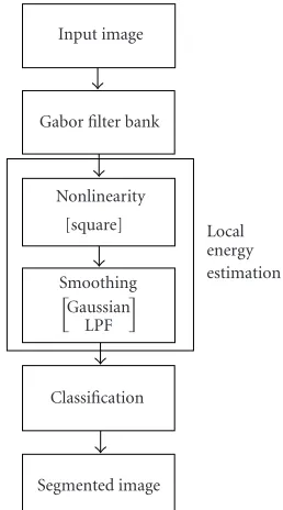
General multichannel filtering methods as shown in Figure 2consist of three major stages: usage of the filter bank to generate filtered images, local energy estimation for fea-ture extraction, and classification of extracted feafea-tures into different regions for segmentation [14]. In the first step, a textured input image is decomposed into filtered images. Typically, in the second stage, a local energy function con-sisting of nonlinearity and smoothing is applied on the fil-tered images (the output of the Gabor filter bank) for feature extraction [1,3,10,11]. The most well-known nonlinearity
Segmented image Classification
Smoothing
Gaussian LPF
Nonlinearity [square] Gabor filter bank
Input image
Local energy estimation
Figure2: Multichannel decomposition process.
Segmented image Classification of quantized vectors
by MLP Feature vector
reduction by CN
Weight vectors after CN is trained High- and low-frequency
components extraction Multichannel decomposition by Gabor filter
Im(x, y)
Figure3: GCN method.
3. GABOR FILTER BANK IN CONJUNCTION
WITH COMPETITIVE NETWORK (GCN)
The first proposed method (GCN) as shown inFigure 3 con-sists of the following stages: multichannel decomposition, high- and low-frequency component extraction, computing features, feature vector reduction, and classification by mul-tilayer perceptron. The detail of each stage is described in this section.
3.1. Multichannel decomposition
This stage consists of filtering by a Gabor filter bank, applying a nonlinearity function, and smoothing the results. We used three sets of Gabor filters composed of 20, 30, and 40 filters. For all sets, the same five radial frequencies suggested by Jain and Farrokhnia [3], that is, 4√2, 8√2, 16√2, 32√2, 64√2, are used.
The radial frequency bandwidth is one octave, thus the frequency difference of f1andf2 is given by log2(f2/ f1), and
is equal to 1. In the first bank for each radial frequency, four orientations 0◦, 45◦, 90◦, and 135◦are used to generate the total number of 20 channels. In the second bank, six orien-tations 0◦, 30◦, 60◦, 90◦, 120◦, and 150◦are used that give a bank of 30 filters, and the third one composed of 40 filters is obtained by eight orientations for each radial frequency, that is, 0◦, 22.5◦, 45◦, 67.5◦, 90◦, 112.5◦, 135◦, and 157.5◦.
The filter banks consisting of 20 and 30 filters using 45◦ and 30◦ orientations, respectively, were used widely in pre-vious research [3,4,11,12]. Here we introduce the third fil-ter bank using 22.5◦ angular bandwidths and orientations. In several experiments with a variety of different textures us-ing all three filter banks, we computed the preserved energy in the filtered images. By comparing and sorting the filtered images according to the preserved energies, we observed that by dividing the angular bandwidth by two, that is, 22.5◦in place of 45◦and covering the frequency domain by this
angu-lar bandwidth, not only could we catch the textures with 45◦ orientations, that is, 0◦, 45◦, 90◦, and 135◦, but also we could better discriminate and classify textures with 22.5◦ orienta-tions, that is, 0◦, 22.5◦, 67.5◦, 112.5◦, and 157.5◦. It was no-ticed that for some textures, maximum energy is preserved by filters with 45◦orientations (and 22.5◦angular bandwidths) and filters with 22.5◦orientations (and 22.5◦angular band-widths). By applying 22.5◦ orientations for different radial frequencies and sorting the filtered images regarding pre-served energies, we obpre-served that some of the filtered images with these orientations are among the ten best filters with re-spect to the preserved energy of the original image. Hence, for this filter bank, we used eight equally spaced orientations 0◦, 22.5◦, 45◦, 67.5◦, 90◦, 112.5◦, 135◦, and 157.5◦and to en-sure proper coverage of the spatial-frequency domain, we set the angular bandwidth to 22.5◦. Orientations and radial fre-quencies of the ten best filters using the three mentioned fil-ter banks are presented inTable 1. The best filters are selected and sorted according to the preserved energies. The results are obtained by applying three Gabor filter banks to a com-plex synthetic textured image depicted inFigure 4.
In the second step, a square function is applied to achieve nonlinearity and it causes the sinusoidal modulations in the output of a filter bank to be transformed to a square modula-tion. To smooth out the fluctuations in the specific texture or noise in the image “Im(x,y),” a Gaussian lowpass filter is ap-plied to the output of the filter bank. The size of the smooth-ing function is determined accordsmooth-ing to the size of the Gabor bandpass filter. The impulse response of the Gaussian filter is
h(x)=√1
2πσ ·exp
−1
2
x2
σ2
, (6)
where σ = 1/2√2f0 and f0 is the radial frequency of the
bandpass Gabor filter.
3.2. High- and low-frequency component extraction
As depicted inFigure 5, neither this filter bank having 40 Ga-bor filters nor the two other GaGa-bor filter banks with 20 and 30 filters completely cover the corners of the frequency do-main along the diagonals. The coverage of the Gabor filter banks are not perfectly flat, thus there are some regions that are not covered and as a result do not have a flat response, in-cluding very high-frequency and very low-frequency regions. In the proposed method, the spatial implementation of the Gabor filter bank is optimized by considering the diagonal high-frequency and very low-frequency components.
The low frequency components that are not included in the Gabor filter bank are obtained by (4) where radial frequency f0is equal to zero and concludes a Gaussian
low-pass filter as follows:
h2(x,y)=g(x,y)·cos
2π f0x
=g(x,y). (7)
Table1: Radial frequencies and orientations of the 10 best filters of the 3 filter banks.
Filter bank Radial frequency and orientation of 10 best filters
1: angular band width=45◦ 64√2 & 90◦, 64√2 & 135◦, 64√2 & 0◦, 64√2 & 45◦, 32√2 & 90◦, 32√2 & 0◦, 32√2 & 135◦, 32√2 & 45◦, 16√2 & 0◦, 16√2 & 45◦
2: angular band width=30◦ 64
√
2 & 90◦, 64√2 & 150◦, 64√2 & 0◦, 64√2 & 120◦, 64√2 & 60◦, 32√2 & 90◦, 64√2 & 30◦, 32√2 & 0◦, 32√2 & 60◦, 32√2 & 150◦
3: angular band width=22.5◦ 64 √
2 & 90◦, 64√2 & 157.5◦, 64√2 & 135◦, 64√2 & 67.5◦, 64√2 & 112.5◦, 64√2 & 0◦, 32√2 & 90◦, 64√2 & 45◦, 64√2 & 22.5◦, 32√2 & 67.5◦
Figure 4: Textured image composed of Asphalt.0000, Misc.0002, Grass.0002, and Concrete.0001 selected from MeasTex Image Tex-ture Database.
Each high-frequency component is computed by
hd(x,y)=Im(x,y)∗δ(x,y)−h2(x,y)∗Im(x,y)
− L
1
h1(x,y)∗Im(x,y),
(8)
where hd(x,y) is the diagonal high-frequency component
and is equal toh(x,y)∗Im(x,y),h1is the Gabor filter
im-pulse response,Lis the Number of filters in the filter bank, andh2is the Gaussian lowpass impulse response.
3.3. Computing features
To compute the feature vector for each pixel of the input im-age, the mean and variance are computed over a neighbor-hood window of the pixel [17]. Mean and variance are reli-able attributes of textures and have small variations over the same texture when the window size is accurately selected to cover the texture periodicity. According to the periodicity of the textures in the input image, the size of the neighborhood window could change and be determined by the user. For tex-tured images with smaller periodicity, the window centered by the regarded pixel would be smaller and would select the larger window for the textures with larger periodicity. In the experiments, window sizes from as small as 4 by 4 to as big as 32 by 32 pixels are used depending on texture periodicity.
3.4. Feature vector reduction by
competitive networks
Grouping several neurons in a single layer [18,19] forms a competitive network. Each neuron is a single processing ele-ment that shares its processing functions with other neurons
Figure5: A bank of 40 Gabor filters.
and responds to a group of input vectors in a different clus-ter maximally. This layer of neurons can classify any input vector, since the neuron with the strongest response for a given input identifies the cluster to which the input vector is most likely to belong. Since, for this layer there is no ex-ternal judge to decide which neuron wins, the neurons must decide this by themselves [18,19] by using an unsupervised learning method. This decision-making process needs com-munication among all neurons in the layer.
To reduce the feature vector dimension a competitive network is used. In the competitive layer the neurons are distributed in order to recognize frequently presented input vectors in an unsupervised manner. The competitive trans-fer function accepts a net input for each neuron in the layer and returns neuron outputs of 0 for all neurons except for the winner, which outputs 1. In a competitive layer each neuron competes to respond to an input vectorp; the neuron whose weight vector is closest to pgets the highest net input and, therefore, wins the competition and outputs 1 and all other neurons output 0.
In the training phase, the winner is moved closer to the input by adjusting the weights of the winning neuron [18] with the learning rule as shown by
∆w=λ(p−w), (9)
Segmented image Classifier Gaussian LPF(x, y) Square
h1(x, y) hd(x, y) h2(x, y)
Classification Smoothing Nonlinearity
Gabor filter
Diagonal high frequency Low frequency Input image
Figure6: Optimized filter bank.
likely to win if a very different input vector is provided. Dur-ing trainDur-ing, as more inputs are presented, each neuron in the layer closest to a group of input vectors adjusts its weights to more closely resemble the inputs. Eventually, every cluster of similar input vectors will have a neuron that identifies the presented vector if it belongs to the cluster and the competi-tive network will categorize the input vectors.
To reduce the feature dimension in the GCN method, a competitive network (CN) as depicted in Figure 7 is used. The motivation to use competitive networks stems from the previous research using LVQ for classification [4,18]. LVQ consists of one competitive layer and one linear layer, and it is a supervised learning algorithm. LVQ describes the class bor-ders by the nearest neighbor rule and its main applications are in statistical pattern recognition and classification [18]. Despite using a hidden competitive layer, LVQ is restricted by only learning linear relationships between quantized vec-tors and desired output vecvec-tors. If the network could learn the nonlinear relationships between the reduced dimension vectors and desired outputs, improved segmentation results would possibly be obtained .
On the other hand, applying the resultant weight vec-tors of a competitive layer to the features prior to feeding the classifier would reduce the dimensionality of feature vec-tors as depicted inFigure 7and faster segmentation would result. In order to train CN, sample vectors are selected at random among the extracted feature vectors obtained by the Gabor filter bank in the previous step. After CN is trained, the weight vectors of the layer are regarded as quantizing mask coefficients. These coefficients are the optimum ex-tracted features of the Gabor filter bank. To select the num-ber of neurons in the network that is equal to the numnum-ber of the most important eigenvectors, 42 neurons (the total
num-w1r . . .
w11 w2r . . .
w21 w1r . . .
w11
p3
. . .
pr
p2 p1
. . .
. . .
. . . Training
feature vectors 42×1
n1 n2 n1
f
a1 a2 a1
Weight vectors of competitive layer 21×42
(a) Weight vectors of converged competitive network 21×42 Feature vectors extracted by Gabor filter bank 42×1
21×1 quantized feature vectors
Multilayer perceptron
Segmented image
(b)
Figure7: Feature reduction and classification by GCN method.
ber of possible eigenvectors) are selected as the initial value, then the layer is trained with training samples and the clas-sification error for the network is computed. By pruning the neurons in the network, repeating the same approach, and computing the classification error, the appropriate number of neurons in the layer is chosen. In our competitive network according to the classification error and dimension of quan-tized feature vectors, 21 neurons are selected for CN as the optimum number of neurons. After selecting the appropri-ate number of neurons, the competitive layer will be trained and the estimated eigenvectors (i.e., weight vectors of the net-work) are obtained and regarded as quantizing mask coeffi -cients. These coefficients are applied on the extracted feature vectors by the Gabor filter bank. The resultant weight vectors of a competitive layer are applied to the features prior to feed-ing in the classifier and will reduce the dimensionality of fea-ture vectors.
3.5. Classification by multilayer perceptron
often have one or more hidden layers of sigmoid neurons fol-lowed by an output layer [19]. The MLP is trained by adjust-ing the weights usadjust-ing least-square error (LSE) that minimizes the mean square error as shown by
E=
N 1
Rk−Ok
2
N . (10)
The total square error between the desiredRk class and the
actual outputOkis calculated forNneurons in output layer
K. To train the neural network, the gradient is determined by using a backpropagation technique which involves per-forming computations backwards through the network. Af-ter the backpropagation network is trained properly, it typ-ically provides reasonable answers when presented with in-puts that it has never seen. Commonly, a new input vector similar to past inputs used during training leads to an out-put similar to correct values. A 3-layer perceptron, which is used to accomplish the segmentation task, is depicted in Figure 7. Our MLP uses the sigmoid transfer function in all three layers. During training, randomly selected quantized feature vectors are assigned to proper classes. Although there are 42 filters in the filter bank, the quantized feature dimen-sion is 21. After MLP is trained, input images will be seg-mented by assigning quantized feature vectors to proper re-gions.
CN and MLP are used in the proposed method for feature dimension reduction and classification, respectively; there-fore we need a two-stage training process. In the first stage, an unsupervised learning using unlabeled samples is employed to train the competitive network. As an efficient approach to compute principle component analysis (PCA), the weight vectors of the trained network are applied to the extracted Gabor features before classification. In the second stage, a su-pervised learning is employed to train the MLP, that is, clas-sifier, by labeled samples. Although in this stage the same set of training samples as of the first stage are used, the label of each sample is also required to train MLP. Using labeled sam-ples, MLP adjusts its weight vectors such that it can effectively recognize all different classes (labels). Despite having two in-dependent training stages, the classification performance of MLP depends on how precise CN approximates PCA which in turn depends on training samples and initialization of the weight vectors.
4. ADAPTIVELY SELECTED GABOR FILTER BANK
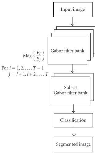
The number of filters in a filter bank affects classification per-formance and has a crucial importance. Much research has been conducted to reduce the number of required filters in the Gabor filter bank for segmentation. In this section, an al-gorithm is presented to select an optimized subset of the Ga-bor filter bank. The proposed method as depicted inFigure 8 consists of three stages: (1) image decomposition, (2) subset filter selection, and (3) classification. The decomposition and classification stages are the same as the first approach; hence the second stage is explained in the following section.
Segmented image Classification
Subset Gabor filter bank Gabor filter bank
Input image
Max
Ei
Ej
Fori=1,2, . . . , T−1
j=i+ 1, i+ 2, . . . , T
Figure8: Adaptive filter selection.
4.1. Selection of a subset bank of the Gabor filters In this approach, a set of Gabor filters are selected as the best Gabor filters, so that each single Gabor filter in this small set of selected Gabor filters can discriminate a pair of textures in an image with multiple textures. Assume that an input image I consists ofT different textural classes Tc,c = 1, 2,. . .,T,
and letIc, a subimage ofI, be a training sample of the texture
classTc. Furthermore, assume thatEiis the preserved energy
of the texture classi.The optimal Gabor filter set is selected based on the energy ratio of each distinct texture pairTiand
Tj,i=j:
Ei
Ej
, i=1, 2,. . .,T−1, j=i+ 1,i+ 2,. . .,T. (11)
Therefore, the optimal filter set is given by
Maximum
Ei
Ej
, i=1, 2,. . .,T−1, j=i+ 1,i+ 2,. . .,T.
(12)
In this approach, the best Gabor filters are selected so that the corresponding energy ratio is maximum for each pair of distinct textures in a multiple-textured image. For instance, having an image composed of two different texture classes Ti = 1 andTj =2, the filter set includes only one filter to
discriminate these two textures and has the maximum energy ratio as Maximum{E1/E2}.
To choose the best filter by obtaining the maximum en-ergy ratio, the enen-ergy ratioEi/Ejis calculated for all 40 Gabor
frequencies:
4√2, 8√2, 16√2, 32√2, 64√2. (13)
The 40 obtained energy ratios are sorted accordingly and the filter which has the maximum ratio among them is selected for each pair of textures:
E1
E2
f
, f =1, 2,. . ., 40, (14)
E1
E2
i
>
E1
E2
j
>· · ·>
E1
E2
k
, (15)
where,i,j,k=1, 2,. . ., 40 andi=j,i=k,j=k.
The energy ratio Ei/Ej of each texture pair Ti and Tj,
i = j, for an image containing T different textures is cal-culated on each filtered image and sorted in decreasing order so that the maximum ratio is achieved according to (12). The larger the value of ratioEi/Ej, the better the discrimination
of distinct texture pairiand j. Thus the best discriminative filter for each pair of different textures according to the max-imum energy ratio is selected to be included in the subset filter bank:
findex∈SFB{Subset Filter Bank},
if
Ei
Ej
index
>
Ei
Ej
k
∀k∈1, 2,. . ., 40, index=k,
fori=1, 2,. . .,T−1;j=i+ 1,i+ 2,. . .,T.
(16)
The subset filter is composed ofNfilters:
N=T×(T−1)
2 . (17)
For instance the size of subset filter for an image containing 4 different textures is
T=4=⇒N=4×(4−1)
2 =6. (18)
5. RESULTS
In several experiments, three sets of filters are used consisting of 20, 30, and 40 filters with 45◦, 30◦, and 22.5◦orientations, respectively. Applying the first method, the segmented results are obtained using 40 filters with 22.5◦angular bandwidths. Two new low-frequency and high-frequency filters are added to improve the filter bank. This raises the total number of filters in the filter bank to 42. The increase in the feature di-mension by using 42 filters in comparison with 20 and 30 filters in the previous published reports is compensated by feature quantization using competitive network. The dimen-sion of quantized feature vectors is 21 and it may change de-pending on the number of textures in the image, that is, if we have less than 4 textures in the input image, we could use a smaller dimension for quantized vectors. In the second ap-proach to segment the textured images, a subset filter bank is adaptively selected. The Gabor filters which compose this
subset filter are selected so that in a multiple texture image, the energy ratio of any two distinct textures is maximum. The number of filters in this subset is variable and depends on the number of textures in the image.
In this section, some results obtained by applying the proposed approaches and three widely used approaches for texture segmentation including Gabor, discrete cosine trans-form (DCT), and Laws filters are presented. Since the Gabor filter was outperformed in comparison with the Laws and DCT in previous research [4], optimized Gabor filter banks will be compared with these filter banks to evaluate the per-formance of the proposed methods. As it was explained in Section 4.1, Ng et al. [5] introduced a 3 by 3 DCT to ex-tract features from textured images. They suggested using eight masks excluding the low-frequency component of the DCT. On the other hand, Laws introduced a separable fil-ter bank to identify different textures for texture segmenta-tion. The suggested filter bank by Laws [6] is composed of 25 filters including five filters in each dimension. These one-dimensional kernels are
L5=[1, 4, 6, 4, 1], E5=[−1,−2, 0, 2, 1], S5=[−1, 0, 2, 0,−1], W5=[−1, 2, 0,−2, 1],
R5=[1,−4, 6,−4, 1].
(19)
By applying the filter bank to the input image, 25 filtered im-ages are produced. These mnemonics (L, E,S,W, andR) stand for level, edge, spot, wave, and ripple. Note that all ker-nels except forL5 have zero sums.
We have obtained the results by applying our proposed methods, Gabor, DCT, and Laws filters, to the synthetic tex-tured images. The segmentation results are compared for five filter banks and are presented in the following section.
5.1. Synthetic textured images
To test the algorithm, a set of synthetic textured im-ages formed by selected textures from the Brodatz al-bum [20], MIT Vision and Modeling Database (see http://vismod.media.mit.edu/vismod), and MeasTex Image Texture Database (see http://www.cssip.uq.edu.au/meastex/ meastex.html) are used. We used combinations of 2, 3, 4, and 5 textures as test images. The sample synthetic images consist of D77, D84, D55, D53, D24, and D17 selected from the Brodatz album; Fabric.0000, Fabric.0017, Flowers.0002, Leaves.0006, and Leaves.0013 selected from MIT Vision and Modeling Database; and Grass.0002, Misc.0002, and Rock.0005 selected from MeasTex Image Texture Database.
(a) (b) (c)
(d) (e) (f)
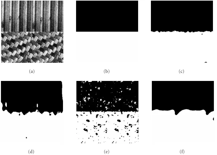
Figure9: (a) Texture image. (b) The true segmentation reference image. (c) Segmentation results by GCN method; classification error is 0.59%. (d) Segmentation results by AGFB; classification error is 2.57%. (e) Segmentation results by DCT; classification error is 2.91%. (f) Segmentation results by Laws filters; classification error is 3.42%.
Table2: Classification errors forFigure 8.
Method Classification error
GCN 0.59%
AGFB 2.57%
DCT 2.91%
Laws 3.42%
Gabor 3.56%
and the Gabor filters, respectively. The GCN improves the classification results by 80% and 91% in comparison with the DCT and Laws filters, respectively. These amounts are 12% and 58% for AGFB.
The image depicted in Figure 10a is a textured im-age consisting of Fabric.0000, Fabric.0017, Flowers.0002, Leaves.0006, and Leaves.0013 selected from MIT Vision and Modeling Database. Figure 10b is the true segmentation reference imag. Figure 10c shows the segmented result by GCN method andFigure 10dshows the segmented result by AGFB. The segmented results by Laws and DCT are depicted in Figures10eand10f, respectively.
The comparison of the classification errors using our proposed methods and the segmentation results using Ga-bor, DCT, and Laws filters for textured image of Figure 10 are shown inTable 3. The proposed GCN method improved the classification results by 45% and 79% in comparison with DCT and Laws filters, respectively. These amounts are 12% and 58% for AGFB.
According to the results obtained in this study which are shown inTable 3, and the previous research, the proposed approaches have better classification performances in
com-parison with the other three methods, that is, Gabor, DCT, and Laws filter bank. The filter parameters for different filter banks which are used for image segmentation are shown in Table 3. As depicted inTable 3, the number of filters for Ga-bor, DCT, and Laws are equal to the feature dimension and are 20, 8, and 25, respectively. In GCN, despite having 42 fil-ters in the filter bank, the feature dimension is reduced to 21 and in AGFB, the number of filters is adaptively selected.
6. DISCUSSION AND CONCLUSION
(a) (b)
(c) (d)
(e) (f)
Figure10: (a) Textured image. (b) The true segmentation reference image. (c) Segmentation results by GCN method; classification error is 8.37%. (d) Segmentation results by AGFB; classification error is 12.62%. (e) Segmentation results by Laws filters; classification error is 25.7%. (f) Segmentation results by DCT; classification error is 15.27%.
Table3: Number of filters and features forFigure 9.
Method Segmentation improvement (percent) No. of filters No. of features
GCN 8.37 42 21
AGFB 12.62 10 10
DCT 15.27 8 8
Laws 25.7 25 25
Gabor 27.5 20 20
The proposed segmentation algorithms are formulated as a combinational optimum approach to obtain a better filter bank, to reduce feature dimension, and to improve classification. The main advantages of the proposed methods include the following:
(1) the proposed approaches allow to use a larger filter bank consisting of a higher number of channels; (2) both methods permit the use of a larger number of
fil-ter banks while the process compensates for the weak-ness of a specific filter bank in some frequencies; (3) the feature quantization and classification component
of this algorithm is a generic approach with the ability to learn and process different kinds of input vectors (feature vectors);
(4) both methods are capable of segmenting complex tex-tured images.
proposed methods are reasonable and almost as complex as DCT and Laws filters. Among these five filter banks, AGFB is the fastest because of its small number of filters. As a tradeoff between the speed and classification error, both of our pro-posed methods offer more than a 50% improvement in clas-sification. GCN takes almost the same computation time as 20 Gabor filters. Although the GCN method reduces the fea-ture dimension using principal component analysis, imple-menting PCA by means of a competitive network speeds up the algorithm and is much faster than the conventional PCA. Designing the Gabor filter bank by accurate parameter selection and using a different learning method according to the specific segmentation problem may improve the accuracy of this algorithm to get better segmentation results based on the nature of the input images. Minimizing the number of filters for texture discrimination has crucial importance and is still an area of active research. Thus, improving the AGFB method would be part of the future work. The algorithm may also be extended to problems such as biomedical and satel-lite image segmentation. Our current goal is to improve the performance of this algorithm and, in future research, apply the proposed techniques to segmentation of satellite and syn-thetic aperture radar (SAR) texture images.
REFERENCES
[1] A. C. Bovik, M. Clark, and W. S. Geisler, “Multichannel tex-ture analysis using localized spatial filters,”IEEE Trans. Pattern Anal. Machine Intell., vol. 12, no. 1, pp. 55–73, 1990. [2] D. F. Dunn and W. E. Higgins, “Optimal Gabor filters for
tex-ture segmentation,”IEEE Trans. Image Processing, vol. 4, no. 7, pp. 947–964, 1995.
[3] A. K. Jain and F. Farrokhnia, “Unsupervised texture segmen-tation using Gabor filters,”Pattern Recognition, vol. 24, no. 12, pp. 1167–1186, 1991.
[4] T. Randen and J. H. Husoy, “Filtering for texture classifica-tion: a comparative study,”IEEE Trans. Pattern Anal. Machine Intell., vol. 21, no. 4, pp. 291–310, 1999.
[5] I. Ng, T. Tan, and J. Kittler, “On local linear transform and Gabor filter representation of texture,” in Proc. 11th IAPR International Conference on Pattern Recognition (ICPR ’92), pp. 627–631, the Hague, the Netherlands, August–September 1992.
[6] K. I. Laws, “Rapid texture identification,” inConference on Im-age Processing for Missile Guidance, vol. 238 ofProceedings of SPIE, pp. 367–380, San Diego, Calif, USA, July 1980. [7] D. A. Pollen and S. F. Ronner, “Visual cortical neurons as
lo-calized spatial frequency filters,”IEEE Trans. Syst., Man, Cy-bern., vol. 13, no. 5, pp. 907–916, 1983.
[8] J. G. Daugman, “Uncertainty relation for resolution in space, spatial frequency, and orientation optimized by two-dimensional visual cortical filters,”Journal of the Optical Soci-ety of America{A}, vol. 2, no. 7, pp. 1160–1169, 1985. [9] M. Unser and M. Eden, “Nonlinear operators for
improv-ing texture segmentation based on features extracted by spa-tial filtering,”IEEE Trans. Syst., Man, Cybern., vol. 20, no. 4, pp. 804–815, 1990.
[10] T. P. Weldon, W. E. Higgins, and D. F. Dunn, “Gabor filter de-sign for multiple texture segmentation,”Optical Engineering, vol. 35, no. 10, pp. 2852–2863, 1996.
[11] D. A. Clausi and M. Ed Jernigan, “Designing Gabor filters for optimal texture separability,”Pattern Recognition, vol. 33, no. 11, pp. 1835–1849, 2000.
[12] A. K. Jain and K. Karu, “Learning texture discrimination masks,” IEEE Trans. Pattern Anal. Machine Intell., vol. 18, no. 2, pp. 195–205, 1996.
[13] T. P. Weldon and W. E. Higgins, “Design of multiple Gabor fil-ters for texture segmentation,” inProc. IEEE Int. Conf. Acous-tics, Speech, Signal Processing (ICASSP ’96), vol. 4, pp. 2245– 2248, Atlanta, Ga, USA, May 1996.
[14] A. C. Bovik, “Analysis of multichannel narrow-band filters for image texture segmentation,”IEEE Trans. Signal Processing, vol. 39, no. 9, pp. 2025–2043, 1991.
[15] J. Strand and T. Taxt, “Local frequency features for texture classification,”Pattern Recognition, vol. 27, no. 10, pp. 1397– 1406, 1994.
[16] R. O. Duda and P. E. Hart,Pattern Classification and Scene Analysis, John Wiley & Sons, New York, NY, USA, 1973. [17] J. Beck, “Textural segmentation, second-order statistics, and
textural elements,”Biol. Cybernetics, vol. 48, no. 2, pp. 125– 130, 1983.
[18] T. Kohonen, Self-Organizing Maps, Springer-Verlag, Berlin, Germany, 1997.
[19] J. A. Freeman and D. M. Skapura,Neural Networks: Algo-rithms, Applications and Programming Techniques, Addison-Wesley, Reading, Mass, USA, 1992.
[20] P. Brodatz,Textures: a Photographic Album for Artists and De-signers, Dover Publications, New York, NY, USA, 1966.
Nezamoddin N. Kachouiereceived his B.S. degree in computer engineering from Isfa-han University of Technology (IUT) in 1989 and his M.S. degree in electrical and com-puter engineering from Ryerson University in 2003. Currently he is a Ph.D. candidate at the University of Waterloo. His research area is biomedical video segmentation and tracking. Currently he is modeling and de-signing an automatic-model-based
segmen-tation and tracking system with the applications of multicellular microscope cell images. He is interested in deformable models and Bayesian framework for biomedical applications of multiple-target tracking. His research interests include object tracking, spatio-temporal image analysis, image denoising, optimization, and clas-sification, and applications of fuzzy logic, neural networks, and ge-netic algorithms in image processing.
Javad Alirezaiereceived his B.S. degree in electrical and electronic engineering from Tehran University in 1988 and his M.A.Sc. and Ph.D. degrees in systems design engi-neering from the University of Waterloo in 1993 and 1996, respectiv+ely. From 1997 to 2000, he was a Postdoctoral Fellow, an As-sistant Professor, and an R&D Fellow in a private sector. He joined Ryerson University in 2001. He is currently an Assistant