R E S E A R C H
Open Access
Performance analysis for time-frequency MUSIC
algorithm in presence of both additive noise and
array calibration errors
Mohamed Khodja
1*, Adel Belouchrani
1and Karim Abed-Meraim
2Abstract
This article deals with the application of Spatial Time-Frequency Distribution (STFD) to the direction finding problem using the Multiple Signal Classification (MUSIC)algorithm. A comparative performance analysis is performed for the method under consideration with respect to that using data covariance matrix when the received array signals are subject to calibration errors in a non-stationary environment. An unified analytical expression of the Direction Of Arrival (DOA) error estimation is derived for both methods. Numerical results show the effect of the parameters intervening in the derived expression on the algorithm performance. It is particularly observed that for low Signal to Noise Ratio (SNR) and high Signal to sensor Perturbation Ratio (SPR) the STFD method gives better performance, while for high SNR and for the same SPR both methods give similar performance.
1 Introduction
Advances in antennas technology and signal processing have allowed the emergence of the generation of “the so-called” smart antennas. The latter are commonly used for the direction of arrival (DOA) estimation of far field sources from multiple antenna outputs. DOA esti-mation is currently one of the important issues in next generation wireless communications, namely the space division multiple access (SDMA).
The techniques used in DOA estimation depend on the nature of the signals under consideration. When the impinging signals are stationary, conventional methods such as the eigen-subspace decomposition of the covar-iance data matrix are usually used [1,2]. These methods lose of their performance for non-stationary signals. Other high resolution techniques like the ones based on the spatial time-frequency distributions (STFD) were introduced to cope with the non-stationary nature of the signals [3-6]. STFD based methods are based on the use of the quadratic time-frequency distributions of the received signals at the array antenna. High resolution DOA estimation consists of applying the eigen-subspace
decomposition of the STFD instead of the conventional covariance data matrix. In [7], performance comparison between the Time-Frequency MUSIC (TF-MUSIC) and the conventional MUSIC, in presence of additive noise, is provided. In [8], statistical performance analysis in presence of sensor errors without considering the pre-sence of observation noise are conducted for DOA esti-mation algorithms based on second-order statistics (SOS). In [9], first-order perturbation analysis of the conventional SOS MUSIC and root-MUSIC algorithms is presented.
In this article, our interest is focused on the perfor-mance analysis of the conventional MUSIC and the TF-MUSIC algorithms in the presence of both additive noise and sensor errors. These errors can incorporate the effect of imprecisely known sensor location, pertur-bations in the antenna amplitude and phase patterns that we consider as the calibration errors. A unified ana-lytical expression of the DOA error estimation is derived for both methods. An analysis of the effect of the sensor perturbations on the performance of the considered algorithms is also provided.
Notations
In this article, boldface symbols are used in lower-case letters for vectors (e.g.,a), and in upper-case letters for * Correspondence: [email protected]
1
Electrical Engineering Department, Ecole Nationale Polytechnique, Algiers, Algeria
Full list of author information is available at the end of the article
matrices (e.g., A). The principal symbols and notations used are listed below.
K number of signal sources
L number of sensors
M number of snapshots
θk kth direction of arrival
a(θk) kth steering vector
A(θ) array response matrix
I L×Lidentity matrix (.)* complex conjugate of (.)
(.)H complex conjugate transpose of (.)
Tr(.) trace of (.)
δi,k Kronecker delta function.
2 Data model
We consider a uniform linear array (ULA) ofLsensors receiving Kincident signals. The data vector at the out-put of the sensors at timetis given by,
y(t) =A(θ)s(t)+n(t) (1)
This model is commonly used in array signal proces-sing, wherey(t) = [y1(t) ...yL(t)]Tis the output array vec-tor, withyi(t),i= 1, ...,L, the output of theith sensor.A (θ) = [a(θ1) ... a(θK)] is the L ×K structured mixing matrix known as the array steering matrix, each vector
a(θj), j= 1, ..., K, is an array response to a signal sj(t) from direction θj.n(t) = [n1(t) ...nL(t)]T is an additive noise that we assume to be a zero mean white complex
stationary process with covariance matrix
Rnn=E[n(t)nH(t)] =σn2I, ands(t) = [s1(t) ...sK (t)]T is the source signal vector with covariance matrix Rss=E [s(t)sH (t)]. The source signals si(t), i = 1, ..., K, are assumed mutually uncorrelated and frequency modu-lated signals of the form
si(t) =Siejϕi(t) (2)
where Siandi(t) are the amplitude and phase of the
ith source signal. The amplitude Si is assumed to be a random variable with zero mean and variance σs2i, while the phasei(t) is time varying.
When the sensors are subject to perturbations due to errors in calibration or in sensor location, the signal response is corrupted by errors characterized by the vec-tors {ai}Ki=1 added to the steering vectors {a(θi)}Ki=1.
Theses errors are randomly changing from one observa-tion period to another. Furthermore, we assume that these errors are uncorrelated random variables with zero mean and equal variances σ2a. The disturbed array manifold matrix can then be written as,
˜
A(θ) =A(θ) +A (3)
This is a widely used disturbance model [8-12] that take into account different sensor errors including those related to calibration. According to Equations (1) and (3), the disturbed data model is,
˜
y(t)=[A(θ)+A]s(t)+n(t) (4)
and can be expressed under the form
˜
y(t) = y◦(t) +p(t) (5)
where y◦(t) is the perturbation free data matrix, and p (t) is the perturbation vector including the sensor errors and the additive noise assumed uncorrelated,
◦
y(t) =A(θ)s(t) (6)
p(t) =As(t) +n(t) (7)
3 Covariance matrix perturbation
The covariance matrix of (5) is given by,
R˜y˜y=E[y˜(t)y˜H(t)]
=E[(y◦(t) +p(t))(y◦H(t) +pH(t))]
(8)
Substituting p(t) with its expression (7) into (8), and sinceΔAis zero mean (E[ΔA] =E[ΔAH] = 0), it results that,
Ry˜y˜ =E[y◦(t)y◦
H
(t)] +E[As(t)sH(t)AH] +σn2I (9)
whereIis theL×Lidentity matrix, and,
E[y◦(t)y◦H(t)] =A(θ)E[s(t)sH(t)]AH(θ)
=A(θ)RssAH(θ)
(10)
where Rss=E[s(t)sH(t)] = diag[σs21, ...,σ
2
sK]. It is pro-ven in Appendix 1 that the second term in the Equation (9) is given by,
E[As(t)sH(t)AH] =σ2aTr(Rss)I (11)
where Tr(Rss)=
K
i=1 σ2
si. Substituting (10) and (11)
into (9), the covariance matrix of the perturbed data can then be written as,
Ry˜y˜ =A(θ)RssAH(θ) + [σ2aTr(Rss) +σn2]I (12)
4 STFD matrix perturbation
diversity provided by the multi-sensor platform. In this article, we consider the discrete form of the spatial pseudo Wigner-Ville distribution (PWVD) matrix using a rectangular window of odd lengthNthat we apply to the perturbed data y˜(t) vector,
Dy˜y˜(t,f) =
(N−1)/2
τ=−(N−1)/2
˜
y(t+τ)y˜H(t−τ)e−j4πfτ (13)
Substituting (5) into (13) we obtain,
Dy˜y˜(t,f) =Dy◦y◦(t,f) +Dy p◦ (t,f) +Dp◦y(t,f) +Dpp(t,f) (14)
D◦
y◦y(t,f) is the STFD data matrix in absence of the
sensor error and the additive noise, and Dpp is the per-turbation STFD matrix, while D◦
y p and Dpy◦ are the
cross STFDs matrices. Under the property of zero mean of noise n(t) and sensor error represented byΔA, the expectation of the cross-terms vanishes (i,e., E[D◦
yp] = 0
and E[Dpy◦] = 0), and it follows,
E[Dy˜y˜(t,f)] =E[D◦
y◦y(t,f)] +E[Dpp(t,f)] (15)
Considering the spatially and temporally white assumptions of the perturbed steering matrix and noise, and using Equations (6) and (7) the above equation becomes,
E[D˜y˜y(t,f)] =E[D◦
y˙y(t,f)] +E[ADss(t,f)A H] +E[D
nn(t,f)] (16)
Where
E[Dnn(t,f)] =σn2I (17)
and
D◦
yy◦(t,f) =A(θ)Dss(t,f)A(θ)
H
(18)
Dss(t,f) is aK×Ksource signal STFD matrix whose elements are given by,
dsisk(t,f) =SiSk
(N−1)/2
τ=−(N−1)/2
ej[ϕi(t+τ)−ϕk(t−τ)−4πfτ] (19)
where the diagonal elements dsisi(t,f) are the auto-TFDs of the source signals, while the off-diagonal ele-ments dsisk(t,f), (i=k), are the cross-TFDs. We con-sider only the t-f points along the actual instantaneous frequency (IF) of each signal. Furthermore, assuming a second-order approximation of the derivative of the phase, we have,
ϕi(t+τ)−ϕi(t−τ)−4πfi(t)τ = 0 (20)
where the IFfi(t) is given by,
fi(t) = 1 2π
dϕi(t)
dt (21)
Therefore, it results from (19) that,
E[dsisi(t,f)] =Nσ
2
si (22)
In order to exploit the STFD given by (13) under an eigen-decomposition form, we use an averaging method which consists of averaging the STFD matrix Dy˜y˜(t,f)
at (ti, fi) points over the selected sources and over a number ofToselected tf-points (To=M -N+ 1), where
Mis the number of snapshots.
¯
Dy˜y˜ =
1
KTo K
k=1 To
i=1
Dy˜y˜(ti,fk,i) (23)
whose expectation is given by,
E[D¯˜yy˜] =
1
KTo K
k=1 To
i=1
E[Dy˜y˜(ti,fk,i)] (24)
where fk,i is the IF of thekth signal at theith time sample. Considering the Equation (14) for the (ti, fk,i) points and substituting it into (23), we obtain, after a straightforward calculation carried out in Appendix 2, the following expression,
ˆ
Dy˜y˜=E[D¯y˜y˜] =
N
KA(θ)RssA
H(θ) +
N
Kσ
2
aTr(Rss) +σn2
I(25)
5 Perturbation analysis: unified formulation
Expressions of R˜y˜y and Dˆ˜yy˜ given by (12) and (25),
respectively, are a sum of three terms corresponding to the perturbation free signal, the sensor error, and the additive noise. These expressions can be written under a unified form as follows,
Py˜y˜ =Py◦◦y+σp2I (26)
where,
P◦
yy◦= ⎧ ⎨ ⎩
R◦
y◦y=A(θ)RssAH(θ), for covariance based method,
ˆ
D◦
yy◦= N KA(θ)RssA
H(θ), for STFD based method (27)
ˆ
D◦
y◦y is the STFD matrix corresponding to the sources
in absence of both noise and sensor errors, and,
σ2 p =
⎧ ⎨ ⎩
(σsos p )
2
=σ2
aTr(Rss) +σn2, for covariance based method,
(σptf) 2
=N Kσ
2
aTr(Rss) +σn2, for STFD based method
In Equation (28), the superscript “sos“stands for sec-ond-order statistics associated to the covariance matrix based method, and the superscript“tf“ stands for time-frequency associated to the STFD based method.
Remarks
•It is important to observe from Equation (25) that in absence of additive noise, the STFD based method do not make any improvement compared to the conventional MUSIC.
• On the other hand, in presence of additive noise, as it is always the case in a real-life situation, the sig-nal to noise ratio (SNR) is improved by a factorN/K for the STFD based method. This improvement would be still better for larger window length.
According to (26) and (27), P˜y˜y is a positive definite
matrix and can be expressed under an eigen-decomposi-tion form as follows,
P˜y˜y=
˜
Usos˜sos(U˜sos)H, for covariance based method, ˜
Utf˜tf(U˜tf)H, for STFD based method (29)
which can be expressed under the following unified form
Py˜y˜ =
L
i=1
λiu˜iu˜Hi =U˜˜U˜ H
(30)
where ˜ = diag[λi,i= 1, . . . , L] is the matrix of the
eigenvalues of Py˜y˜, and u˜i
L
i=1 are the corresponding
eigenvectors.
These definitions and notations being made, and for the sake of simplicity we consider in the sequel only the unified form P˜y˜y given by Equation (30) to deal with
both the covariance and the STFD based methods. The matrix U˜ can be arranged as U˜ = [U˜s U˜p],
where U˜s= [u˜1,. . . ,u˜K] forms the signal subspace, and
˜
Up= [u˜K+1,. . .,u˜L] forms the perturbed subspace
known as the orthogonal subspace. The Equation (30) can then be rewritten as follows,
Py˜y˜ =
˜
UsU˜p
˜ s 0
0 ˜p
˜
UHs
˜
UHp
=U˜s˜sU˜ H
s +U˜p˜pU˜ H p
(31)
where ˜s = diag[λi, i= 1, . . . , K] is the signal
eigenvalue matrix, and ˜p= diag[λi, i=K+ 1, . . . , L]
the perturbation eigenvalue matrix. Thus, consequently to (31), a perturbation Py˜y˜ leads to the perturbation of
both subspaces. The matrices U˜s and U˜p can then be
expressed as,
˜
Us=Us+Us and U˜p=Up+Up (32)
where ΔUsand ΔUp represent, respectively, the per-turbation of the signal subspace and the orthogonal subspace.
It is shown in Appendix 3 that the first-order expres-sions forΔUsandΔUpare given by,
Us=Up+UpHPyyUs −s1 (33)
Up=−Us −s1UHs PHyyUp (34) ΔPyy represents the perturbation resulting from the presence of sensor errors and the additive noise in the data signal,
Pyy=
Ryy, for covariance based method,
Dyy, for STFD based method (35)
where,
Ryy=
1
M
˜
y(t)y˜(t)H−y◦(t)y◦(t)H (36)
and,
Dyy=
1
KTo K
k=1 To
i=1
[Dy˜y˜(ti,fk,i)−Dy˙y◦(ti,fk,i)] (37)
6 DOA error estimation for the MUSIC and TF-MUSIC algorithms
In the MUSIC and TF-MUSIC algorithms, the DOA are found by locating the Klargest peaks over the angle of arrivalθof the following spatial spectrum function,
F(θ) =a(θ)HU˜pU˜ H
pa(θ) (38)
In a perturbed environment, the direction of arrivals {θk}Kk=1 are corrupted by the errors {θk}Kk=1. Thus, the kth estimated DOA corresponding to thekth signal can be written as,
˜
θk=θk+θk (39)
and the expression for the perturbation of DOA esti-mate, proved in Appendix 4, is given by,
θk=
Re [−a(θk)HUpUHpa(1)(θk)]
a(1)(θk)HU p2
a(1)(θk) =da(θ)
dθ θ=θk, k= 1, ...,K. SubstitutingΔUpby its expression given in (34), we obtain,
θk=
Re[a(θk)HUs −s1UHs PHyyUpUHpa(1)(θk)]
a(1)(θk)HU p2
(41)
which can be written under the following form [1],
θk=
Re [αkHPHyyβk]
γk
(42)
where the vectorsakandbkare given by,
αk=Us −s1UHs a(θk) (43)
βk=UpUHpa (1)
(θk) (44)
and the scalargkis given by,
γk= ||a(1)(θk)HUp||2 (45)
The variance of the kth DOA error estimate Δθk is then given by,
var (θk) = 1 γ2
k
var [Re (αkHPHyyβk)] (46)
Taking into account the notations given in the pre-vious section, the results (41) and (46) are valid for both the conventional and time-frequency MUSIC.
var [θk] =
var [θsos
k ], for conventional MUSIC algorithm
var [θktf], for TF-MUSIC algorithm (47)
where,
var [θksos] = 1 (γsos
k )
2var [Re ((α sos k )
HRH
yyβksos)] (48)
and
var [θktf] = 1 (γktf)2
var [Re ((αtfk)HDHyyβktf)] (49)
7 Performance evaluation
In this section, simulation results are given for the STFD and the SOS MUSIC methods. Two received chirp source signals are considered,s1(t) =S1exp[j((w12
-w11)(t2/2) +w11t)] ands2(t) =S2exp[j((w22- w21)(t2/2) +
w21t)] with powers σs21 = 1 and σs22 = 4, and with fre-quencies varying from w11 =π/6 to w12 =π and from
w21=πtow22=π/6, respectively. The signals are posi-tioned at anglesθ1 = -10° andθ2 = 10° and are received
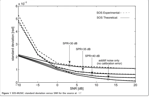
by a uniform linear array of eight sensors spaced by half-wavelength. The signal at the output of the array is disturbed by calibration errors in addition to the addi-tive noise. These perturbations are assumed uncorre-lated Gaussian variables with zero mean. In all simulations, we limit our discussion to small calibration errors and consider the signal to perturbation ratio (SPR) for the values 30, 35, and 40 dB. In the STFD based method, a PWVD with rectangular window length of 129 is applied to the sensor output data. The observa-tion period is 1024 snapshots and the results are aver-aged over 500 independent Monte Carlo trials. DOA estimates θ˜1 and θ˜2 are obtained for each Monte Carlo run by locating the peaks of the spectrum and compar-ing them toθ1andθ2, respectively. The variance of the differences θ1=θ˜1−θ1 and θ2=θ˜2−θ2, constitute
the simulation results. As for numerical results related to the variance terms in Equations (48) and (49), they are obtained by Monte Carlo method.
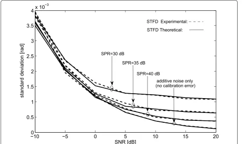
Figures 1, 2, 3, and 4 show the statistical performance of each method versus the SNR for different values of the SPR. The curves in these figures compare the empirical standard deviation with the theoretical expres-sions shown by (48) and (49). The results presented in Figures 1 and 3 are obtained using Δθ1, whereas the results presented in Figures 2 and 4 are obtained for Δθ2. As we can see from Figures 1 and 2, the simulation results for the SOS-based method agree closely with the results of the derived analytical expression for SNR≥ 0 dB. The same observation is made for the STFD-based method from Figures 3 and 4 but for a larger range of SNRs. We can also observe that for the SOS-based method the matching between empirical and theoretical results is lost for very low SNR values (i.e., SNR <0) due to the fact that the first order disturbance analysis is not pertinent in this context. However, for the STFD-based method, the matching between empirical and theoretical results still hold because the local SNR value at the auto-source time-frequency point is relatively large even at SNR = -10 dB. This robustness with respect to noise may be explained by the effect of spreading the noise power over the time-frequency plan and of localizing the source energy in the t-f domain. Moreover, as shown in the above referenced equations, this result is supported by the SNR improvement of a factor equal to the t-f window length N over the SNR associated to SOS based method.
−010 −5 0 5 10 15 20 1
2 3 4 5
6x 10
−3
SNR [dB]
stan
dar
d
dev
iat
ion
[ra
d]
additif noise only (no calibration error) SOS Theoretical: SOS Experimental:
SPR=40 dB SPR=35 dB SPR=30 dB
Figure 1SOS-MUSIC: standard deviation versus SNR for the source at-10°.
−
0
10
−
5
0
5
10
15
20
0.5
1
1.5
2
2.5
x 10
−3
SNR [dB]
stan
dar
d
dev
iat
ion
[ra
d]
additif noise only (no calibration error) SOS Theoretical:
SOS Experimental:
SPR=40 dB SPR=35 dB
SPR=30 dB
−010 −5 0 5 10 15 20 0.5
1 1.5 2 2.5 3 3.5
4x 10
−3
SNR [dB]
standard deviation [rad]
additive noise only (no calibration error) STFD Experimental:
SPR=40 dB SPR=35 dB SPR=30 dB
STFD Theoretical:
Figure 3STFD-MUSIC: standard deviation versus SNR for the source at-10°.
−010 −5 0 5 10 15 20
0.5 1 1.5 2
2.5x 10
−3
SNR [dB]
standard deviation [rad]
additive noise only (no calibration error) STFD Experimental:
SPR=40 dB SPR=35 dB
SPR=30 dB
STFD Theoretical:
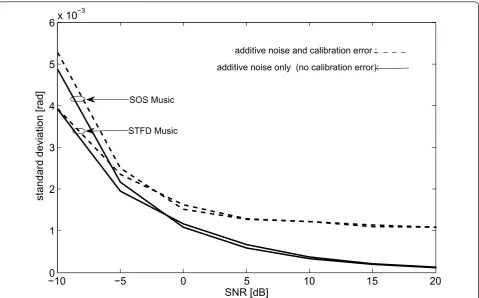
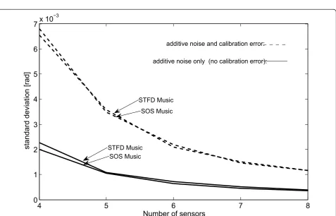
dB) the STFD-based method significantly outperforms the SOS-based one. This difference, as shown in Figures 6 and 7, is further affected by the number of sensors which is a parameter of resolution and thus of perfor-mance. It is clear from these figures that more the num-ber of sensors is large, better is the performance of the algorithms. Figure 6 shows the improvement carried out by the STFD-based method in presence of high additive noise (SNR = -10 dB). As expected from data model (4) and Equation (28), it is observed in this figure that the presence of small calibration errors (SPR = 30 dB) have no significant effect on both methods and all occurs as if there were only the presence of the additive noise. However, as shown in Figure 7, the presence of weak noise with the same calibration error value as in the previous figure, produce a significant performance degradation and the two methods become equivalent.
8 Conclusion
The STFD-based direction finding and covariance matrix-based methods have been considered and a uni-fied analytical expression of the DOA error estimation have been derived for both methods. It is shown that in presence of calibration errors and large additive noise the STFD-based method has better performance than
the SOS-based method, and that in presence of weak noise both methods are equivalent in their performance. However, even for small sensor perturbations, degrada-tion in performance remains significant because of the multiplicative character of the perturbation with the sig-nal. Through the results obtained in this article, it clearly appears that the TF-MUSIC algorithm plays an important role in the performance improvement, how-ever the implementation of this algorithm may be use-less if the sensors are already at the outset too badly calibrated.
Appendix 1: Proof of Equation (11)
Herein, we derive the expression of (11) given by,
E[As(t)sH(t)AH] (1:1)
Before calculate this expression, we start by defining the matrixΔAand the vectors(t) as,
A= ⎡ ⎢ ⎢ ⎢ ⎣
a1,1a1,2· · · a1,K a2,1a2,2· · · a2,K
..
. ... . .. ... aL,1aL,2· · · aL,K
⎤ ⎥ ⎥ ⎥
⎦ands(t) = ⎡ ⎢ ⎢ ⎢ ⎣
s1(t) s2(t)
.. .
sK(t) ⎤ ⎥ ⎥ ⎥ ⎦ (1:2)
−010 −5 0 5 10 15 20
1 2 3 4 5
6x 10
−3
SNR [dB]
standard deviation [rad]
additive noise only (no calibration error): additive noise and calibration error :
SOS Music
STFD Music
4 5 6 7 8 0
0.01 0.02 0.03 0.04 0.05 0.06 0.07
Number of sensors
stan
dar
d
dev
iat
ion
[ra
d]
additive noise only (no calibration error): additive noise and calibration error :
STFD Music SOS Music
Figure 6SOS and STFD-MUSIC: standard deviation versus the number of sensors for low SNR (= -10dB) and small calibration errors (SPR = 30 dB).
4 5 6 7 8
0 1 2 3 4 5 6
7x 10
−3
Number of sensors
standard deviation [rad]
additive noise only (no calibration error): additive noise and calibration error:
STFD Music SOS Music
STFD Music SOS Music
and omitting the argumenttofskfor brevity, we get,
E[As(t)sH(t)AH] =E
K
i=1 a1,isi
K
i=1 a2,isi. . .
K
i=1 aL,isi
T
×
⎡ ⎣K
j=1 a∗1,js∗j
K
j=1
a∗2,js∗j. . . K
j=1 a∗L,js∗j
⎤ ⎦ ⎫ ⎬ ⎭
(1:3)
Since the source signalssi, i= 1, ...,K, and the sensor errors Δai,j, j= 1, ..., L, are assumed independent and zero mean with variances σs2i and σ2a, respectively, the above expression is anL×Lmatrix whose elements are given by,
σp,q= K i=1 K j=1
E[ap,ia∗q,jsis∗j]
= K i=1 K j=1
E[ap,ia∗q,j]E[sis∗j]
=σ2a
⎛
⎝K
j=1 σ2
si
⎞ ⎠δp,q
(1:4)
Therefore, the matrix given by (1.1) is a diagonal matrix which can be expressed as,
E[As(t)sH(t)AH] =σ2
a K i=1 σ2 si
I=σ2
aTr(Rss)I (1:5)
Appendix 2: Proof of Equation (25)
Herein, we derive the expression of (25),
E[D¯˜y˜y] =
1 KTo K k=1 To i=1
E[Dy˜y˜(ti,fk,i)] (2:1)
Considering equation (16) for thekth source signal at the (ti,fk,i) points, and substituting it into (2.1) we have,
E[D¯y˜˜y] = 1
KTo K k=1 To i=1
E[akdsksk(ti,fk,i)a
H
k] +E[akdsksk(ti,fk,i)a
H k] +σn2I
(2:2)
Taking into account (22) we obtain,
E[D¯y˜y˜] =
1 KTo K k=1 T o i=1
Nσs2kaka
H k +Nσ
2
skE[aka
H k] +σ
2 nI % =N K K k=1 σ2
skaka
H k +σs2kσ
2 aI
+σ2
nI =N K K k=1 σ2
skaka
H k +N Kσ 2
aTr(Rss)I+σn2I
=N KA(θ)RssA
H(θ) +
N
Kσ
2
aTr(Rss) +σn2
I
(2:3)
where Rss=E[s(t)sH(t)] = diag[σs21, . . . , σ
2 sK] and
Tr(Rss) =K i=1σ
2 si
Appendix 3: Proof of Equations (33) and (34)
According to (31) we have,
P˜y˜y=U˜s˜sU˜
H
s +U˜p˜pU˜ H
p (3:1)
Multiplying both sides of Py˜y˜ by the matrices U˜Hp and ˜
Us and using the orthogonality property between these
matrices, it follows,
˜
UHpPy˜y˜U˜s= 0 (3:2)
that we can write as,
(Up+Up)H(P◦
yy◦+Pyy)(Us+Us) = 0 (3:3)
Expanding the above equation and neglecting the terms higher than the first-order perturbation, and, on another hand, considering relation (27) and the ortho-gonality property between the signal subspace and the orthogonal subspace, it follows,
UHpPyyUs+UpHPy◦y◦Us= 0 (3:4)
since the eigenvalue decomposition of the perturba-tion free matrix is given by P◦
y◦y=Us sU
H
s , and using
the unitary property of Us(i.e.,UHs Us=I), we get,
UHp =−UHpPyyUs[Us s]# (3:5)
where [.]# defines the pseudo-inverse operator, hence
[Us s]# is given by,
[Us s]#= [(Us s)H(Us s)]−1(Us s)H
= −s1UHs (3:6)
Substituting (3.6) in (3.5), we obtain,
Up=−Us −s1UHs PHyyUp (3:7)
Using the same steps applied to derive the above equation, we obtain the expression of the signal sub-space perturbationΔUsversus the perturbation matrix ΔPyy,
Appendix 4: Proof of Equation (40)
Herein, we derive the expression (40) of the estimate of the errorΔθk, k= 1, ...,K, due to the sensor error and the additive noise. For this purpose, we use the extre-mum search method which consists of finding the zeros of the derivative of the objective function derived from the estimated orthogonal subspace,
F(θ) =a(θ)HU˜pU˜ H
pa(θ) (4:1)
A well known method is to expand under Taylor ser-ies the first partial derivative of the above function with respect toθand to use a second-order approximation to extractΔθk,
∂F(θ˜k)
∂θ =
∞
n=0 1
n!
∂n+1F(θ
k)
∂θn+1 (θk)
n
=∂F(θk)
∂θ + ∂2F(θ
k)
∂θ2 θk+ . . . + 1
i!
∂i+1F(θ
k)
∂θi+1 θ
i k+ . . . ,
(4:2)
that we approximate by the two first terms,
∂F(θ˜k)
∂θ ≈
∂F(θk)
∂θ +
∂2F(θk)
∂θ2 θk (4:3)
Setting the above equation to zero leads to the follow-ing expression ofΔθk,
θk≈ − ∂F(θk)
∂θ ∂2F(θk)
∂θ2
, k= 1, ...,K (4:4)
where,
∂F(θk) ∂θk
=a(1)(θk)HU˜pU˜ H
pa(θk) +a(θk)HU˜pU˜ H
pa(1)(θk) (4:5)
and,
∂2F(θ
k)
∂θ2
k =a(2)(θ
k)HU˜pU˜ H
pa(θk) + 2a(1)(θk)HU˜pU˜ H
pa(1)(θk) +a(θk)HU˜pU˜ H
pa(2)(θk), (4:6)
the superscripts (1) and (2) correspond to the first and the second-order derivatives of a(θ) with respect to θ, respectively.
Substituting U˜p=Up+Up in the above equations,
and using the property of orthogonality between the subspaces spanned bya(θk) andUp(i.e., a(θk)H Up= 0), and neglecting the derivatives and the perturbation terms of second-order, we obtain,
∂F(θk) ∂θk
= 2Re [a(θk)HUpUHpa(1)(θk)] (4:7)
and
∂2F(θ k) ∂θ2
k
= 2a(1)(θ
k)HUpUHpa(1)(θk) + 2Re [a(1)(θk)HUpUHpa(1)(θk)] (4:8)
Assuming that ΔUp =εUp, where ε ≪ 1, the above equation can be written as,
∂2F(θk) ∂θ2
k
= 2(1 +ε)a(1)(θk)HUp2
≈2a(1)(θk)HUp2
(4:9)
Substituting (4.7) and (4.9) into (4.4), it results the expression of the perturbation in the kth estimated direction of arrival as follows,
θk=
Re [−a(θk)HUpUHpa(1)(θk)]
a(1)(θ
k)HUp2
(4:10)
Author details
1Electrical Engineering Department, Ecole Nationale Polytechnique, Algiers, Algeria2Télécom ParisTech, TSI, 75634, Paris Cedex 13, France
Competing interests
The authors declare that they have no competing interests.
Received: 17 October 2011 Accepted: 30 April 2012 Published: 30 April 2012
References
1. F Li, H Liu, RJ Vaccaro, Performance analysis for DOA estimation algorithms: unification, simplification, and observations. IEEE Trans. Aerosp. Electron. Syst.29(4), 1170–1183 (1993)
2. P Stoica, A Nehorai, MUSIC, Maximum Likelihood, and Cramer-Rao Bound. IEEE Trans. Acoustics Speech Signal Processing.37(5), 720–741 (1989) 3. A Belouchrani, M Amin, Time-frequency MUSIC. IEEE Signal Process. Lett.6,
109–110 (1999)
4. A Belouchrani, M Amin, A new approach for blind source separation using time-frequency distribution, inProceeding SPIE Conference on Advanced Algorithms and Architectures for Signal Processing, vol. 2846. Denver, Colorado, pp. 193–203 (Oct 1996)
5. B Belouchrani, M Amin, Blind source separation based on time-frequency signal representations. IEEE Trans. Signal Process.46(11), 2888–2898 (1998) 6. B Boashash,Time-Frequency Signal Analysis and Processing: A Comprehensive
Reference, (Elsevier Science Publ, San Diego, 2003)
7. Z Yimin, M Weifeng, M Amin, Subspace analysis of spatial time-frequency distribution matrices. IEEE Trans. Signal Process.49(4), 747–759 (2001) 8. F Li, RJ Vaccaro, Sensitivity analysis of DOA estimation algorithms to sensor
errors. IEEE Trans. Aerosp. Electron. Syst.28(3), 708–717 (1992) 9. AL Swindlehurst, T Kailath, A performance analysis of subspace-based
methods in the presence of model errors, Part I: the MUSIC algorithm. IEEE Trans. Signal Process.40(7), 1758–1774 (1992)
10. AL Swindlehurst, A maximum a posteriori approach to beamforming in the presence of calibration errors, inProc. 8th IEEE Workshop Stat. Signal Array Process, Corfu, Greece, pp. 82–85 (June 1996)
11. J Yang, AL Swindlehurst, The effect of array calibration errors on DF-based signal copy performance. IEEE Trans. Signal Process.43(11), 2724–2732 (1995)
12. C Vaidyanathan, KM Buckley, Performance analysis of the MVDR spatial spectrum estimator. IEEE Trans. Signal Process.43(6), 1427–1437 (1995)
doi:10.1186/1687-6180-2012-94