Determination of the Strong Coupling Constant by the ALPHA
Collaboration
TomaszKorzec1,for the ALPHA collaboration
1Department of Physics, Bergische Universität Wuppertal, Gaußstr. 20, 42119 Wuppertal, Germany
Abstract. A high precision determination of the strong coupling constant in the MS scheme at the Z-mass scale, using low energy quantities, namely pion/kaon decay con-stants and masses, as experimental input is presented. The computation employs two different massless finite volume renormalization schemes to non-perturbatively trace the scale dependence of the respective running couplings from a scale of about 200 MeV to 100 GeV. At the largest energies perturbation theory is reliable. At high energies the Schrödinger-Functional scheme is used, while the running at low and intermediate ener-gies is computed in a novel renormalization scheme based on an improved gradient flow. Large volumeNf=2+1 QCD simulations by CLS are used to set the overall scale. The
result is compared to world averages by FLAG and the PDG.
1 Introduction
Parameters of the standard model have to be determined experimentally before any predictions can be made. Improvements in the knowledge of these fundamental quantities translate into a higher predic-tive power of the model and are crucial for the successful operation of expensive collider experiments like the LHC. A parameter that is most important and so far not particularly precisely determined is the coupling in the strong sector of the standard model. The difficulties in its determination lie in the confining properties of QCD. The typical method to measure it is to “fit” the perturbative prediction of a high energy process to the corresponding measurement. In order for the truncated perturbative series to describe the process well, one is forced to concentrate on processes where the physical en-ergy scale of the process is high, i.e. µ1 GeV. Only then the QCD coupling is small enough and truncation errors are under control. The main uncertainties are systematic errors associated with the necessary processing of the raw data, before it can be compared to perturbation theory. To infer what fundamental process has taken place from the measured energies and momenta of photons, leptons and hadrons, one relies not only on a detailed mathematical model of the detector, but also on a good understanding of the hadronization process. The latter is too complicated to be computed within the standard model and various model assumptions enter which in the end may dominate the system-atic error. Furthermore many experiments rely on a set of measured structure functions, which can introduce subtle correlations in the results of different collaborations.
A summary of the methods and most precise experimental determinations is compiled regularly by the particle data group [1]. The different results are combined into a world average, its most recent
τ-deca
ys
la
ttic
e
struc
tur
e
func
tions
e
+
e–
jets & shapes
hadron collider electroweak precision fits Baikov
ABM BBG JR MMHT NNPDF Davier Pich Boito SM review HPQCD (Wilson loops)
HPQCD (c-c correlators)
Maltmann (Wilson loops)
Dissertori (3j)
JADE (3j)
DW (T)
Abbate (T)
Gehrm. (T)
CMS
(tt cross section)
GFitter Hoang
(C)
JADE(j&s)
OPAL(j&s)
ALEPH (jets&shapes)
PACS-CS (SF scheme)
ETM (ghost-gluon vertex)
BBGPSV (static potent.)
April 2016
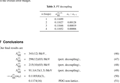
Figure 1.The left panel is PDG’s [1] summary ofαSdeterminations. The yellow bands correspond to the
pre-averages of different classes of determinations. The right panel, by FLAG [2], focuses on determinations that
used lattice QCD as a tool. The gray bands are the global averages of the two groups.
value beingαS(MZ)=0.1181(11). This is the MS-coupling of the five flavor theory renormalized at
µ=MZ,αS(µ)≡
¯
g(5)
MS(µ)
2
/(4π). In recent years lattice QCD has become increasingly important as a tool that allows to connect low and high energy regimes non-perturbatively. The couplingαS(MZ)
can then be determined from measured values of low energy hadronic quantities like pion masses and decay constants. Currently some of the world’s most precise determinations are based on lattice QCD and already dominate the world average. The latest status is summarized in Fig.1. Lattice deter-minations are also reviewed and averaged by the Flavour Lattice Averaging Group [2]. The current FLAG average includes results from [3–7]. Most of the uncertainties in these lattice determinations are systematic in nature and are rooted in the multi-scale nature of the problem. On the one hand the spatial extentLof the simulated box needs to be large enough to avoid finite volume effects in hadronic observables, i.e.Lm−1
π . On the other hand the lattice spacingamust be fine enough to be
able to compute a renormalized coupling at high energiesµ(where it is small). A coupling could for instance be defined through the static force at short distancesr=µ−1, which would requireaµ−1. Insisting on a high value ofµ, e.g. µ ≈100 GeV immediately leads to astronomically large lattice sizesL/a. With today’s machines and algorithms one is restricted to L/a 100 which requires a careful balance of the scalesa,µandLsuch that the unavoidable finite size-, cutoff- and perturbative truncation errors are all under control. For instance the most recent result [7] of Fig.1uses lattices with up toL/a=64 sites, renormalization scalesµ≈5 GeV with lattice spacingsa−1≈3.3 GeV and
coarser.
These systematic errors can be nearly eliminated by switching to finite volume renormalization schemes [8], whereµ≡L−1. The drawback is, that a whole sequence of simulations at various values
τ-deca ys la ttic e struc tur e func tions e + e–
jets & shapes
hadron collider electroweak precision fits Baikov ABM BBG JR MMHT NNPDF Davier Pich Boito SM review HPQCD (Wilson loops)
HPQCD (c-c correlators)
Maltmann (Wilson loops)
Dissertori (3j)
JADE (3j)
DW (T)
Abbate (T)
Gehrm. (T)
CMS
(tt cross section)
GFitter Hoang
(C)
JADE(j&s)
OPAL(j&s)
ALEPH (jets&shapes)
PACS-CS (SF scheme)
ETM (ghost-gluon vertex)
BBGPSV (static potent.)
April 2016
Figure 1.The left panel is PDG’s [1] summary ofαSdeterminations. The yellow bands correspond to the
pre-averages of different classes of determinations. The right panel, by FLAG [2], focuses on determinations that
used lattice QCD as a tool. The gray bands are the global averages of the two groups.
value beingαS(MZ)=0.1181(11). This is the MS-coupling of the five flavor theory renormalized at
µ=MZ,αS(µ)≡
¯
g(5)
MS(µ)
2
/(4π). In recent years lattice QCD has become increasingly important as a tool that allows to connect low and high energy regimes non-perturbatively. The couplingαS(MZ)
can then be determined from measured values of low energy hadronic quantities like pion masses and decay constants. Currently some of the world’s most precise determinations are based on lattice QCD and already dominate the world average. The latest status is summarized in Fig.1. Lattice deter-minations are also reviewed and averaged by the Flavour Lattice Averaging Group [2]. The current FLAG average includes results from [3–7]. Most of the uncertainties in these lattice determinations are systematic in nature and are rooted in the multi-scale nature of the problem. On the one hand the spatial extentLof the simulated box needs to be large enough to avoid finite volume effects in hadronic observables, i.e.Lm−1
π . On the other hand the lattice spacingamust be fine enough to be
able to compute a renormalized coupling at high energiesµ(where it is small). A coupling could for instance be defined through the static force at short distancesr=µ−1, which would requireaµ−1. Insisting on a high value ofµ, e.g. µ ≈ 100 GeV immediately leads to astronomically large lattice sizesL/a. With today’s machines and algorithms one is restricted toL/a 100 which requires a careful balance of the scalesa,µandLsuch that the unavoidable finite size-, cutoff- and perturbative truncation errors are all under control. For instance the most recent result [7] of Fig.1uses lattices with up toL/a=64 sites, renormalization scalesµ≈5 GeV with lattice spacingsa−1≈3.3 GeV and
coarser.
These systematic errors can be nearly eliminated by switching to finite volume renormalization schemes [8], whereµ≡L−1. The drawback is, that a whole sequence of simulations at various values
ofLbecomes necessary. In addition, the results based on finite size scaling were so far plagued by relatively large statistical errors or an insufficient number of dynamical flavors. The only calculation of this type that enters the FLAG average is the one by PACS-CS, [4]. It has a large, but mainly statistical error.
This article summarizes the effort of the ALPHA collaboration to determineαSusing
finite-size-scaling techniques. It is self-contained but, due to size restrictions, many details are omitted. The reader is encouraged to consult the original literature [9–13] for a deeper understanding of the calcu-lation.
The outline of this proceeding contribution is as follows: in Sec. 2 our notation is fixed and basic formulae collected. Sec.3 lays out our computational strategy and the different more or less independent parts of the calculation are treated in some detail in sections4-6. The article concludes with Sec.7where the final result is put together and discussed.
2 Renormalization Schemes and Scales
Almost any renormalized, dimensionless, short-distance quantityφcan be the starting point for the definition of a renormalization scheme. If it possesses a perturbative expansion in a bare couplingg0,
e.g.φ=
l φlg 2l
0, one can define a renormalized coupling in this scheme as ¯g2φ≡ φ−φ0
φ1 . The quantityφ,
the coefficientsφland therefore the renormalized coupling depend on a scaleµ. The scale dependence
of the coupling is expressed by the RG equation
µdg¯
dµ =β(¯g). (1)
Theβfunction depends on the scheme, but in massless schemes the first two coefficients in a pertur-bative expansion
β(¯g)=−¯g3b0+b1g¯2+b2g¯4+. . .
(2) are “universal”
b0= 161π2
11−2N3f
, b1=2561π4
102−383Nf
. (3)
The subsequent coefficients depend on the scheme. They are known to five loops (b2throughb4) in the MS-scheme [14–18] and to three loops (b2) in the SF-scheme [19]. The solution of the ODE Eq. (2)
requires an initial condition, or equivalently, the introduction of aΛ-parameter, e.g. at one loop1
¯
g2(µ)= 1
2b0ln (µ/Λ) or Λ =µe
−1/(2b0g¯2(µ)). (4)
The well known fully non-perturbative expression is
Λ =µb0g¯2(µ)−
b1
2b20 exp
−2b 1
0g¯2(µ)− ¯ g(µ)
0
1
β(x)+
1
b0x3 −
b1 b2 0x dx
. (5)
Λparameters are scheme dependent. Between two schemes with couplings ¯gand ¯gthat are related in perturbation theory by
¯
g2(µ)=g¯2(µ)+cg¯4(µ)+. . . , (6)
the exact relation betweenΛparameters is
Λ= Λec/(2b0). (7)
1Eq. (4) is more of pedagogical than practical value, since it cannot be used to determineΛ, no matter how highµis. It does
Instead of theβ-function, the step-scaling function σ(¯g2) can be invoked to express the scale
dependence of a renormalized coupling. It is defined as the value of the coupling at a renormalization scale that is smaller by a factor of two
σ(u)≡g¯2(µ/2)g¯2(µ)=u. (8)
Both are related by
−ln 2=
√ σ(u)
√u dx
β(x). (9)
The step-scaling function is more directly accessible through computer simulations and plays a central role in our calculation. Its perturbative expansion is
σ(u) = u+s0u2+s1u3+s2u4+. . . (10)
s0 = 2b0ln 2, s1 = (2b0ln 2)2+2b1ln 2, etc. (11)
3 Strategy
Lattice QCD is used as a non-perturbative tool that allows to determine theΛparameter of QCD from low energy experiments.
Our computational strategy can be summarized as follows. In large volume QCD simulations the value of a hadronic quantity, like the pion or kaon decay constant (or, in our case, a linear combination of both, denoted by fπK), is determined at the physical mass point in lattice units on lattices with
different lattice spacings. The experimental measurement of the same quantity2allows to map out a relationship between the bare couplingg0 of the chosen lattice action and the lattice spacing in fm.
At this point one can switch to massless small volume simulations with a known box sizeLhad. A
renormalized coupling ¯g(µ) in a finite volume scheme is defined, in which the renormalization scale is tied to the linear box sizeµ=L−1. Theβfunction of this coupling is determined non-perturbatively for a wide range of couplings, by simulations of lattices with decreasing box sizes. Once the β
function is known, it is used to determine the value of the renormalized coupling at a high energy scaleµ = µPT ≈ 70 GeV, provided that its value atµ ≡ L−1hadis known. At these high energies the
coupling is small and perturbation theory becomes reliable and is used to relate the coupling to theΛ parameter, i.e. a perturbative approximation ofβis used in Eq. (5). This can then be translated exactly
into theΛparameter of a more common scheme. All of this is carried out in massive (Nf =2+1, large volume) or massless (Nf =3, finite volume) QCD. To obtain theΛparameter in four, five or six
flavor QCD, perturbative decoupling [21–26] is invoked.
In practice the above procedure is extended by two steps. The first is to use two different finite volume schemes, each offering significant advantages in the energy region where they are utilized. The couplings of these two schemes are matched non-perturbatively at an intermediate scaleL−1
0 ≈5 GeV.
The other step is to use the flow scalet0[27] as an intermediate scale during the scale-setting, i.e. to
first determine the dimensionless combination oft0 and fπKand then the ratioLhad/√t0. In total the
calculation can be summarized by
Λ(3)
MS=
fPDG πK
fπK√t0
scale setting Sec.4
× √t
0 Lhad connection toL=∞
Sec.5.5
× L2hadL 0 scheme 1 Sec.5.3
× 2LL0 0 change of schemes
Sec.5.4
×Λ(3)
MSL0
scheme 2 Sec.5.2
, (12)
2In pure QCDfπis defined by a matrix element of the axial current between the vacuum and the pion state. Relating this to
Instead of theβ-function, the step-scaling function σ(¯g2) can be invoked to express the scale
dependence of a renormalized coupling. It is defined as the value of the coupling at a renormalization scale that is smaller by a factor of two
σ(u)≡g¯2(µ/2)g¯2(µ)=u. (8)
Both are related by
−ln 2=
√ σ(u)
√u dx
β(x). (9)
The step-scaling function is more directly accessible through computer simulations and plays a central role in our calculation. Its perturbative expansion is
σ(u) = u+s0u2+s1u3+s2u4+. . . (10)
s0 = 2b0ln 2, s1 = (2b0ln 2)2+2b1ln 2, etc. (11)
3 Strategy
Lattice QCD is used as a non-perturbative tool that allows to determine theΛparameter of QCD from low energy experiments.
Our computational strategy can be summarized as follows. In large volume QCD simulations the value of a hadronic quantity, like the pion or kaon decay constant (or, in our case, a linear combination of both, denoted by fπK), is determined at the physical mass point in lattice units on lattices with
different lattice spacings. The experimental measurement of the same quantity2allows to map out a relationship between the bare couplingg0 of the chosen lattice action and the lattice spacing in fm.
At this point one can switch to massless small volume simulations with a known box sizeLhad. A
renormalized coupling ¯g(µ) in a finite volume scheme is defined, in which the renormalization scale is tied to the linear box sizeµ=L−1. Theβfunction of this coupling is determined non-perturbatively for a wide range of couplings, by simulations of lattices with decreasing box sizes. Once the β
function is known, it is used to determine the value of the renormalized coupling at a high energy scaleµ =µPT ≈ 70 GeV, provided that its value atµ ≡ L−1hadis known. At these high energies the
coupling is small and perturbation theory becomes reliable and is used to relate the coupling to theΛ parameter, i.e. a perturbative approximation ofβis used in Eq. (5). This can then be translated exactly
into theΛparameter of a more common scheme. All of this is carried out in massive (Nf =2+1, large volume) or massless (Nf=3, finite volume) QCD. To obtain theΛparameter in four, five or six
flavor QCD, perturbative decoupling [21–26] is invoked.
In practice the above procedure is extended by two steps. The first is to use two different finite volume schemes, each offering significant advantages in the energy region where they are utilized. The couplings of these two schemes are matched non-perturbatively at an intermediate scaleL−1
0 ≈5 GeV.
The other step is to use the flow scalet0[27] as an intermediate scale during the scale-setting, i.e. to
first determine the dimensionless combination oft0and fπKand then the ratioLhad/√t0. In total the
calculation can be summarized by
Λ(3)
MS=
fPDG πK
fπK√t0
scale setting Sec.4
× √t
0 Lhad connection toL=∞
Sec.5.5
× L2hadL 0 scheme 1 Sec.5.3
× 2LL0 0 change of schemes
Sec.5.4
×Λ(3)
MSL0
scheme 2 Sec.5.2
, (12)
2In pure QCDfπis defined by a matrix element of the axial current between the vacuum and the pion state. Relating this to
the experimentally measured values is intricate [20] and to some extent convention dependent.
where each factor is largely independent from the others.
4 Scale Setting
The experimental inputs needed for the determination of the Λ−parameter enter the computation through the process of scale-setting. I.e. the relation between the bare couplingg0 and the lattice
spacing in fm depends on these inputs, for which we take
fπphysK ≡ 23fKphys+1 3f
phys
π = 147.6(5) MeV, (13)
mphysπ = 134.8(3) MeV, (14)
mphysK = 494.2(3) MeV. (15)
The meson masses, corrected for isospin breaking and electro-magnetic effects, are taken from FLAG [2], the decay constants from the PDG [28].
The large-volume simulations were carried out within the “Coordinated Lattice Simulations” consortium (CLS) [9]. The set of ensembles was generated using a tree-level Symanzik improved gauge action [29] and 2+1 flavors of non-perturbatively clover improved [30,31] Wilson fermions. Open boundary conditions in temporal directions made simulations at small lattice spacings, down to a≈0.039 fm possible, without facing problems due to topological critical slowing down [32,33]. All
simulations were carried out using theopenQCDsimulation suite3[34].
Finite lattice spacings and unphysical quark masses make a chiral-continuum extrapolation neces-sary before the scale can be set. It is convenient to use the flow scalet0[27] as an intermediate scale
and to measure
8t0m2π ≡ φ2 ∼mup, (16)
8t0
m2
K+
m2 π
2
≡ φ4 ∼mup+mdown+mstrange, (17)
√t
0fπK, (18)
t0/a2 (19)
on all ensembles. For a precise definition of these observables, bare parameters and choices of plateau regions, we refer the reader to [10]. The parameters of the CLS [9] ensembles were chosen such that
φ4is approximately constant and close to its physical value. Values ofφ2span a range corresponding
to 200 MeV mπ 420 MeV. The simulated bare couplings correspond to four different lattice
spacings between 0.04 fm and 0.09 fm. For the dependence of √t0fπK onφ2and the lattice spacing,
different assumptions can be made. A Taylor expansion around the flavor-symmetric point motivates the ansatz [35]
fTaylor(φ
2,a)=c0+c1(φ2−φsym2 )2+c2 a 2
tsym0 , (20)
while chiral perturbation theory [36,37] suggests
fχPT(φ
2,a)=(√t0fπK)sym
1−7(Lπ−Lsymπ )
6 −
4(LK−LsymK )
3 −
Lη−Lsymη
2 +c4 a
2
tsym0 , (21)
with logarithmsLx= m 2 x
(4πf)2 ln
m2 x
(4πf)2
. These and other functions can be used to read offthe value at
the physical point. The intermediate scale tphys0 in fm is given by tphys0 = f(φphys2 ,0)/fπphysK . The lattice spacings in fm then follow from thet0/a2measurements, extrapolated toφ2=φphys2 .
The value oft0physthat was used to plan the simulations and fix the chiral trajectory was slightly different than the final result of the procedure above. And even if not, the tuning of the ensembles only has a finite precision. Small corrections of the mis-tuning and small changes of the target values are necessary. They can be carried out, if the derivatives of all observables Eq. (16)-Eq. (19) with respect to the bare masses are known. These derivatives are measured as described in [10] and corrections
O(m
0)=O(m0)+(m0−m0)dmdO
0 +O
(m
0−m0)2
(22)
are made until a fixed point in the value oftphys0 is found. Fig.2shows two of the chiral-continuum extrapolations that were attempted after all ensembles were mass-shifted such thatφ4=φphys4 .
0.0 0.1 0.2 0.3 0.4 0.5 0.6 0.7 0.8 φ2
0.100 0.102 0.104 0.106 0.108 0.110 0.112 0.114 0.116
√ t
0
fπ
K
0.00 0.05 0.10 0.15 0.20 0.25 0.30 0.35 0.40 a2/t
0 0.100
0.102 0.104 0.106 0.108 0.110 0.112 0.114 0.116
Figure 2.The left panel shows chiral and continuum extrapolations of √t0fπK. Solid lines correspond to
extrap-olations according to Eq. (20) and dashed lines to Eq. (21). From bottom to top the lattice spacing decreases, the corresponding bare couplings 6/g20are 3.4 (red), 3.46 (green), 3.55 (blue) and 3.7 (black). The extrapolated continuum curve (magenta) is on top. In the right panel it is shown, how well the global fit describes the lattice spacing dependence at the flavor symmetric mass point, where data are available for all lattice spacings.
A further improvement of the procedure above is to replace√t0fπKby
t
0 fπK, wheret0is defined
on the unphysical mass-point wheremup=mdown=mstrangeandφ4=1.11. The advantages are that at
this mass-point simulations are comparatively cheap, no chiral extrapolations oft0/a2are necessary,
finite volume effects are smaller and, by definition, the mass-point remains unchanged, even if in the future, with higher statistics, the values ofφphys2 andφphys4 should change.
Based on the CLS ensembles the procedure sketched above leads to
8t
0 =0.413(5)(2) fm. (23)
with logarithmsLx = m 2 x
(4πf)2 ln
m2 x
(4πf)2
. These and other functions can be used to read offthe value at
the physical point. The intermediate scale tphys0 in fm is given by t0phys = f(φphys2 ,0)/fπphysK . The lattice spacings in fm then follow from thet0/a2measurements, extrapolated toφ2=φphys2 .
The value oft0physthat was used to plan the simulations and fix the chiral trajectory was slightly different than the final result of the procedure above. And even if not, the tuning of the ensembles only has a finite precision. Small corrections of the mis-tuning and small changes of the target values are necessary. They can be carried out, if the derivatives of all observables Eq. (16)-Eq. (19) with respect to the bare masses are known. These derivatives are measured as described in [10] and corrections
O(m
0)=O(m0)+(m0−m0)dmdO
0 +O
(m
0−m0)2
(22)
are made until a fixed point in the value oftphys0 is found. Fig.2shows two of the chiral-continuum extrapolations that were attempted after all ensembles were mass-shifted such thatφ4=φphys4 .
0.0 0.1 0.2 0.3 0.4 0.5 0.6 0.7 0.8 φ2
0.100 0.102 0.104 0.106 0.108 0.110 0.112 0.114 0.116
√ t
0
fπ
K
0.00 0.05 0.10 0.15 0.20 0.25 0.30 0.35 0.40 a2/t
0 0.100
0.102 0.104 0.106 0.108 0.110 0.112 0.114 0.116
Figure 2.The left panel shows chiral and continuum extrapolations of √t0fπK. Solid lines correspond to
extrap-olations according to Eq. (20) and dashed lines to Eq. (21). From bottom to top the lattice spacing decreases, the corresponding bare couplings 6/g20are 3.4 (red), 3.46 (green), 3.55 (blue) and 3.7 (black). The extrapolated continuum curve (magenta) is on top. In the right panel it is shown, how well the global fit describes the lattice spacing dependence at the flavor symmetric mass point, where data are available for all lattice spacings.
A further improvement of the procedure above is to replace √t0fπKby
t
0 fπK, wheret0is defined
on the unphysical mass-point wheremup =mdown=mstrangeandφ4=1.11. The advantages are that at
this mass-point simulations are comparatively cheap, no chiral extrapolations oft0/a2are necessary,
finite volume effects are smaller and, by definition, the mass-point remains unchanged, even if in the future, with higher statistics, the values ofφphys2 andφphys4 should change.
Based on the CLS ensembles the procedure sketched above leads to
8t
0 =0.413(5)(2) fm. (23)
The first error is statistical, the second accounts for uncertainties related to the chiral extrapolations. Different functional forms have been tried and subsets of data neglected/included in order to asses its size [10]. The resulting lattice spacings are summarized in Tab.1.
Table 1.Bare couplings and the corresponding lattice spacings of the CLS ensembles.
6/g20 t
0/a2 ain fm
3.40 2.862(6) 0.086 3.46 3.662(13) 0.076 3.55 5.166(18) 0.064 3.70 8.596(31) 0.050 3.85 14.036(57) 0.039
Table 2.Bare couplings such that ¯
g2GF(L−1
had)=11.31 for variousLhad/a.
6/g20 Lhad/a
3.3998 12.000(58) 3.5498 16.000(30) 3.6867 20.000(83) 3.8000 24.000(105) 3.9791 32.000(153)
5 Running
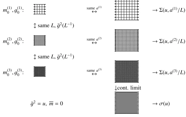
In finite volume renormalization schemes the renormalization scale is tied to the linear box size of the worldµ≡L−1. To determine theβor step-scaling function numerically, a sequence of simulations is
necessary. For instance, to computeσ(u) the necessary steps are sketched in Fig.3. First a lattice
reso-m(1)0 , g(1)0 : same↔a(1) →Σ(u,a(1)/L)
sameL, ¯g2(L−1)
m(2)0 , g(2)0 : same↔a(2) →Σ(u,a(2)/L)
sameL, ¯g2(L−1)
m(3)0 , g(3)0 : same↔a(3) →Σ(u,a(3)/L)
↓cont. limit
¯
g2 =u, m=0 →σ(u)
Figure 3.A sketch of the steps necessary to compute one continuum value of a step-scaling functionσ.
lutionL/ais chosen. Then the bare couplingg0and the bare massm0are tuned such that renormalized
masses are zero, and the renormalized coupling ¯g2 =u. With the same bare parameters another simu-lation with 2L/alattice points in each direction is carried out. Up to lattice artifacts, sameg0implies
same lattice spacing, so the box-size is doubled (or the renormalization scale halved). Measuring the renormalized coupling on the doubled lattice yields a lattice estimate of the step-scaling function Σ(u,a/L). This has to be repeated with the sameu, but finer lattice resolutions, so that a continuum limit can be takenσ(u)= lim
a/L→0Σ(u,a/L). Finally all of this has to be repeated at various values ofu,
Instead of separate continuum extrapolations for eachuand subsequent parametrization ofσ(u),
both can be combined into one step by performing a global fit. A possible ansatz is for instance
Σ(u,a/L)=u+u2
nσ
k=0 skuk+
a L
2nρ
k=1
ρkuk+i+1 (24)
with the lowestsk(up tos1ors2) taken from perturbation theory and the higher left as fit parameters.
Leading lattice artifacts are parametrized by the coefficientsρk and the value ofimay be zero, or
higher, depending on the order in perturbation theory to which the lattice artifacts were removed from the raw data. Different combinations of orders of polynomials (nσ,nρ) can be tried.
A somewhat different approach to fit the data is to choose a parametrization of theβ-function e.g.
β(g) = −g3b0+b1g2+b2g4+. . .
, or (25)
β(g) = − g
3
p0+p1g2+p2g4+. . . (26)
and insert it into Eq. (9). In particular the second choice is interesting, because it leads to a fit that is linear in the fit parameterspk[12]. Making again an ansatz for the leading lattice artifacts the fit
would minimize the violations of the equation
ln 2 = −p0 2
1
Σ(u,a/L)− 1 u
+ p1 2 ln
Σ(u
,a/L)
u
+
np
n=1 pn+1
2n
Σn(u,a/L)−un
+ a
L 2nρ
k=1
ρkuk+i+1, (27)
whereΣ(u,a/L) are the data.
The first choice leads to a non-linear fit, which is feasible if one can get away with very few parametersb3,b4, . . .and takeb0,b1,b2from perturbation theory.
5.1 QCD Schrödinger-Functional
Boundary conditions play a crucial role for finite volume schemes. Depending on the choice simu-lations with massless fermions become more or less expensive, or not possible at all. Schrödinger Functional (SF) boundaries are particularly interesting. They induce a solid spectral gap in the Dirac operator [38], allow to define useful boundary-to-bulk and boundary-to-boundary correlation func-tions [39,40] and can be used to define finite volume couplings with very good properties.
SF boundaries consist of Dirichlet boundaries in time for both fermion and gauge fields, and periodic (up to a phase) boundaries in spacial directions. Gauge fields satisfy
Uk(x)|x0=0=exp(a Ck), Uk(x)|x0=T =exp(a Ck), Uµ(x+Lkˆ)=Uµ(x). (28)
For the choice of boundary gauge fields we restrict ourselves to Abelian SU(3) matrices parametrized by the anglesηandν[41] ,
Ck= i
L
η−π 3
ην−η 2
−ην−η 2 +π3
, Ck= i L −
η−π
ην+η2 +π3
η
2 −ην+23π
(29) For matter fields conditions
1
2[1−γ0]ψ(x)|x0=0=0, 1
Instead of separate continuum extrapolations for eachuand subsequent parametrization ofσ(u),
both can be combined into one step by performing a global fit. A possible ansatz is for instance
Σ(u,a/L)=u+u2
nσ
k=0 skuk+
a L
2nρ
k=1
ρkuk+i+1 (24)
with the lowestsk(up tos1ors2) taken from perturbation theory and the higher left as fit parameters.
Leading lattice artifacts are parametrized by the coefficients ρk and the value ofi may be zero, or
higher, depending on the order in perturbation theory to which the lattice artifacts were removed from the raw data. Different combinations of orders of polynomials (nσ,nρ) can be tried.
A somewhat different approach to fit the data is to choose a parametrization of theβ-function e.g.
β(g) = −g3b0+b1g2+b2g4+. . .
, or (25)
β(g) = − g
3
p0+p1g2+p2g4+. . . (26)
and insert it into Eq. (9). In particular the second choice is interesting, because it leads to a fit that is linear in the fit parameterspk[12]. Making again an ansatz for the leading lattice artifacts the fit
would minimize the violations of the equation
ln 2 = −p0 2
1
Σ(u,a/L)− 1 u
+ p1 2 ln
Σ(u
,a/L)
u
+
np
n=1 pn+1
2n
Σn(u,a/L)−un
+ a
L 2nρ
k=1
ρkuk+i+1, (27)
whereΣ(u,a/L) are the data.
The first choice leads to a non-linear fit, which is feasible if one can get away with very few parametersb3,b4, . . .and takeb0,b1,b2from perturbation theory.
5.1 QCD Schrödinger-Functional
Boundary conditions play a crucial role for finite volume schemes. Depending on the choice simu-lations with massless fermions become more or less expensive, or not possible at all. Schrödinger Functional (SF) boundaries are particularly interesting. They induce a solid spectral gap in the Dirac operator [38], allow to define useful boundary-to-bulk and boundary-to-boundary correlation func-tions [39,40] and can be used to define finite volume couplings with very good properties.
SF boundaries consist of Dirichlet boundaries in time for both fermion and gauge fields, and periodic (up to a phase) boundaries in spacial directions. Gauge fields satisfy
Uk(x)|x0=0=exp(a Ck), Uk(x)|x0=T =exp(a Ck), Uµ(x+Lkˆ)=Uµ(x). (28)
For the choice of boundary gauge fields we restrict ourselves to Abelian SU(3) matrices parametrized by the anglesηandν[41] ,
Ck= i
L η−π 3 ην−η 2 −ην−η 2 +π3
, Ck= i L
−
η−π
ην+η2+π3
η
2−ην+23π
(29) For matter fields conditions
1
2[1−γ0]ψ(x)|x0=0=0, 1
2[1+γ0]ψ(x)|x0=T =0, ψ(x+Lkˆ)=eiθψ(x), (30) and similarly for ¯ψare imposed [42].
5.2 Schrödinger-Functional Coupling
The standard definition of a SF-coupling [41,43] is based on the sensitivity of the effective action
Γ =ln
D[U,ψ, ψ¯ ]e−S[U,ψ,ψ¯ ]
(31)
to the change of boundaries
¯
gν≡k
∂Γ
∂η
η=0
−1
. (32)
This is in fact a whole family of renormalized couplings, the most frequently used one being ¯gSF ≡
¯
gν=0. The normalizationkis chosen such that ¯g2SF=g20+O(g40), [43].
The advantages of coupling Eq. (32) are a good statistical precision, remarkably small lattice artifacts, relatively small computational costs and a good theoretical understanding [19,38]. Itsβ
function is known to three loops. In consequence it has been successfully used for the last quarter century to computeΛ−parameters ofNf =0 [43],Nf =2 [44],Nf =3 [4] andNf =4 [45] QCD and in various beyond-the-standard-model applications, mainly related to a composite Higgs, see e.g. [46] and references therein.
The main disadvantage is that the statistical precision deteriorates at low energies and close to the continuum limit. To leading order, the relative error of ¯g2SFis proportional to ¯g2SF, which makes this scheme particularly useful at higher energies, but problematic when ¯g2SFis large. Moreover the variance of ∂Γ
∂η is not a renormalized quantity. It diverges in the continuum limit [47], which further
increases the costs of the already expensive fine lattices. Here, the SF scheme is used at high energies
5 GeV only.
The step-scaling function of the SF coupling is computed as described in Sec.5 for couplings u∈ {1.1089,1.1845,1.2657,1.3627,1.4808,1.6173,1.7943,2.012}, on lattices withL/a∈ {4,6,8,12}
(and the corresponding doubled lattices). L/a = 4 lattices were excluded from the final analysis, L/a = 12 lattices are available only for a subset of the couplings. The largest coupling implicitly defines the scaleL0at which finite volume schemes are switched
¯
g2SF(L−1
0 )≡2.012. (33)
To be able to make most use of available perturbative results, the lattice action for this part of the project is Wilson’s plaquette action with clover-improved Wilson fermions. For this setup the coeffi-cient of the clover term is known non-perturbatively [48] and the boundary improvement coefficients ct[41] and ˜ct[49] are known to two [19] and one [50] loop respectively. An error due to the limited
knowledge ofctand ˜ctis propagated onto our data and perturbative lattice artifacts are subtracted as
detailed in [11], before trying various fitting procedures.
The left panel of Fig.4shows our data and two possible continuum extrapolations, namely Eq. (24) withnσ=3,i=2 andnρ=2 or 0.
With the non-perturbatively determinedβor step-scaling function at hand it is possible to
deter-mine the coupling at renormalization scalesL−1
0 → 2L−10 → 4L−10 . . .. At stepnEq. (5) can be used
to obtain an estimate of 2−nL
0Λ(3)with a perturbative truncation error, that decreases with growingn.
The situation is depicted in Fig.8. The final result of this part is (see [11] for further details)
L0Λ(3)SF=0.0303(8), or L0Λ(3)MS=0.0791(21). (34)
The well known relation [38] between the SF and the MS schemesΛ(3)SF = 0.38286(2)Λ(3)MS is used
5.3 Gradient Flow Coupling
A recently significantly improved [27, 51–57] understanding of the Yang-Mills gradient flow (GF) [58] has opened the way for the definition of novel scales liket0 [27] orw0 [59] and for the
introduction of new renormalization schemes [60–62].
Correlation functions of fieldsBµ, that are solutions of the gradient flow equation
∂tBµ(t,x) = DνGνµ(t,x), Bµ(0,x)=Aµ(x),
Dµ = ∂µ+[Bµ,·],
Gµν = ∂µBν−∂νBµ+[Bµ,Bν],
were found to be automatically renormalized at flow timest > 0. Simple gauge-invariant
combina-tions, like the action density, can be used in the definitions of couplings and scales, which can then be measured extremely precisely. Moreover their variances are renormalized quantities themselves, such that the continuum limit can be approached without the problem of a diverging noise to signal ratio.
Already in [27] the proposal was made to define a renormalized coupling based on the dimension-less combinationt2Ga
µνGaµν, where the renormalization scale is given by the flow timeµ =1/ √
8t. This original gradient flow renormalization scheme has been recently studied to 2 loops in perturba-tion theory [57]. Different finite volume renormalization schemes, where the flow time (and therefore renormalization scale) are tied to the box sizeµ = 1/L = c/√8t, were invented [60, 61, 63] and successfully applied [64–68]. The variant that is used in this work follows [61]. The running coupling is defined to be
¯
g2GF(µ)=N−1t
2
4
Ga
µν(t,x)Gaµν(t,x)δQ,0 δQ,0
√
8t=cL,x0=T/2
, (35)
whereL = T is the size of a massless Schrödinger functional without background field (C =C = 0),c = 0.3,N a computable normalization factor and the summation overµandνis restricted to the spacial components only. Q = 321π2
d4x
µνρσGaµν(t,x)Gaρσ(t,x) is the topological charge and
a projection onto the trivial sector is included in the definition Eq. (35). This projection reduces the variance and simplifies the error analysis in cases where topological sectors are sampled very slowly [32]. Moreover algorithms can be used, that deliberately stay in the trivial sector [12].
On the lattice a discretization has to be chosen for the action, for the flow equation and for the definition of the observableGa
µν(t,x)Gaµν(t,x). In order to be able to determine the largest simulated
box sizeLhadin fm, defined implicitly by
¯
g2GF(L−1had)≡11.31, (36)
the discretization of the action needs to be the same as the one used by CLS, for which the scale was set. That means, a tree level Symanzik improved gauge action (SLW) and massless clover improved
Wilson fermions. In a finite volume it becomes necessary to specify, how exactly the SF boundary conditions are realized and which values for the boundary improvement coefficientsctand ˜ctare used.
We opt for choice B of ref. [69] for which the coefficients are known to one loop [70,71].
For the discretization of the flow equation and the observable we follow [72] and use the Symazik O(a2) improved lattice flow equation, a.k.a “Zeuthen flow”
a2∂tV µ(t,x)
Vµ(t,x)†=−g20
1+ a
2
12∆µ
∂x,µSLW[V], Vµ(0,x)=Uµ(x). (37)
5.3 Gradient Flow Coupling
A recently significantly improved [27, 51–57] understanding of the Yang-Mills gradient flow (GF) [58] has opened the way for the definition of novel scales liket0 [27] orw0 [59] and for the
introduction of new renormalization schemes [60–62].
Correlation functions of fieldsBµ, that are solutions of the gradient flow equation
∂tBµ(t,x) = DνGνµ(t,x), Bµ(0,x)=Aµ(x),
Dµ = ∂µ+[Bµ,·],
Gµν = ∂µBν−∂νBµ+[Bµ,Bν],
were found to be automatically renormalized at flow timest >0. Simple gauge-invariant
combina-tions, like the action density, can be used in the definitions of couplings and scales, which can then be measured extremely precisely. Moreover their variances are renormalized quantities themselves, such that the continuum limit can be approached without the problem of a diverging noise to signal ratio.
Already in [27] the proposal was made to define a renormalized coupling based on the dimension-less combinationt2Ga
µνGaµν, where the renormalization scale is given by the flow timeµ =1/ √
8t. This original gradient flow renormalization scheme has been recently studied to 2 loops in perturba-tion theory [57]. Different finite volume renormalization schemes, where the flow time (and therefore renormalization scale) are tied to the box sizeµ = 1/L = c/√8t, were invented [60,61,63] and successfully applied [64–68]. The variant that is used in this work follows [61]. The running coupling is defined to be
¯
g2GF(µ)=N−1t
2
4
Ga
µν(t,x)Gaµν(t,x)δQ,0 δQ,0
√
8t=cL,x0=T/2
, (35)
whereL =T is the size of a massless Schrödinger functional without background field (C =C = 0),c = 0.3, N a computable normalization factor and the summation overµandνis restricted to the spacial components only. Q = 321π2
d4x
µνρσGaµν(t,x)Gaρσ(t,x) is the topological charge and
a projection onto the trivial sector is included in the definition Eq. (35). This projection reduces the variance and simplifies the error analysis in cases where topological sectors are sampled very slowly [32]. Moreover algorithms can be used, that deliberately stay in the trivial sector [12].
On the lattice a discretization has to be chosen for the action, for the flow equation and for the definition of the observableGa
µν(t,x)Gaµν(t,x). In order to be able to determine the largest simulated
box sizeLhadin fm, defined implicitly by
¯
g2GF(L−1had)≡11.31, (36)
the discretization of the action needs to be the same as the one used by CLS, for which the scale was set. That means, a tree level Symanzik improved gauge action (SLW) and massless clover improved
Wilson fermions. In a finite volume it becomes necessary to specify, how exactly the SF boundary conditions are realized and which values for the boundary improvement coefficientsctand ˜ctare used.
We opt for choice B of ref. [69] for which the coefficients are known to one loop [70,71].
For the discretization of the flow equation and the observable we follow [72] and use the Symazik O(a2) improved lattice flow equation, a.k.a “Zeuthen flow”
a2∂tV µ(t,x)
Vµ(t,x)†=−g20
1+ a
2
12∆µ
∂x,µSLW[V], Vµ(0,x)=Uµ(x). (37)
Here∂x,µSLWis the force derived from the improved action. For the observable we use the (at finitet) O(a2) improved choice that also entersSLW.
Despite systematically removing several sources ofO(a2) lattice artifacts, the remaining scaling
violations are quite significant, especially when compared to those encountered in the SF scheme. Consequently, finer lattices were necessary for a controlled continuum extrapolation. The data set for this part of the project consists of lattices withL/a∈ {8,12,16}(and doubled lattices) at couplingsu∈ {2.12,2.39,2.74,3.20,3.86,4.48,5.30,5.87,6.55}(approximately). The right panel of Fig.4shows our data and two possible continuum extrapolations.
0 0.005 0.01 0.015 0.02 0.025 1.10
1.12 1.14 1.16 1.18 1.20 1.22
(a/L)2
Σ( u ,a/ L ) /u
1.2 1.4 1.6 1.8 2 2.2
0 0.002 0.004 0.006 0.008 0.01 0.012 0.014 0.016
Σ( u ,a /L ) /u
(a/L)2
FitΣ
Fit1/Σ
Continuum (fitΣ) Continuum (fit1/Σ) Data
Figure 4.Exemplary continuum limits of the step-scaling functions in the SF (left) and the GF (right) schemes. Asterisks in the left plot mark perturbative predictions.
−4.5
−4
−3.5
−3
−2.5
−2
−1.5
−1
−0.5
0
0 0.2 0.4 0.6 0.8 1
β
(
g
)
α=g2/(4π)
Schrödinger Functional Gradient Flow 1-loop 2-loop 3-loop (MS) 4-loop (MS) 5-loop (MS)
0.08 0.1 0.12 0.14 0.16 0.18 0.2−0.3
−0.25
−0.2
−0.15
−0.1
−0.05
0
3-loop (SF)
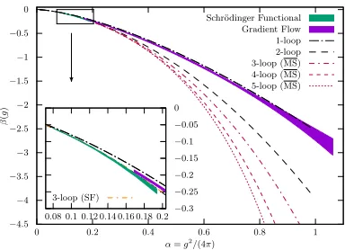
Figure 5. Non-perturbatively determinedβ-functions in the GF and SF schemes and a comparison to various perturbative orders.
Fig.5shows the non-perturbative continuumβfunctions in both schemes in the range of couplings
where they were determined. As expected, in the high energy regime the SFβ-function follows the
5.4 Non-perturbative Matching
Theβfunction of the GF scheme can be used to computeL0in fm, ifLhadin fm is known. To do this,
it is necessary to know the value of the coupling ¯g2GF(L−1
0 ). This is not entirely trivial, becauseL0is
defined implicitly in Eq. (33), i.e. using a different scheme with different boundary conditions and a different lattice action. Since ¯g2GFand ¯g2SFcannot be measured on the same ensembles a (small) set of
new simulations is necessary. The scheme switch is combined with one iteration of step-scaling. For everyL/a∈ {12,16,24,32}with ¯g2SF=2.012 a simulation with the same action, same bare parameters,
doubled linear lattice size and switched offboundary field is carried out. On these doubled lattices ¯
g2GF((2L0)−1) is measured. Finally its continuum limit is obtained, as shown in Fig.6. Its value,
independent of the lattice action, is
¯
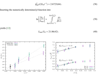
g2GF((2L0)−1)=2.6723(64). (38)
Inserting the numerically determinedβ-function into
ln 2L
0 Lhad
=
¯ gGF(L−had1)
¯ gGF((2L0)−1)
dx
β(x) (39)
yields [12]
Lhad/L0=21.86(42). (40)
2.66 2.67 2.68 2.69 2.7 2.71 2.72 2.73 2.74 2.75 2.76
−0.001 0 0.001 0.002 0.003 0.004 0.005 0.006 0.007
¯
g
2 GF
(2
L
0
)
(a/L)2
Zeuthen flow Wilson flow Continuum
Figure 6. Non-perturbative matching of SF and GF couplings. Continuum extrapolations are shown for the standard (improved) definition of the GF coupling and for one in which the unimproved Wilson flow and an unimproved definition of the observable were used. The smaller error bars stem from ¯g2GF, the complete er-ror bar contains also the contribution due to a finite pre-cision in the tuning to ¯g2SF=2.012.
6.2 6.3 6.4 6.5 6.6 6.7 6.8 6.9 7 7.1 7.2
0 0.05 0.1 0.15 0.2 0.25 0.3 0.35 0.4
g2
GF(Lhad,1) = 11.31
g2
GF(Lhad,2) = 10.20
Lhad
/
√ t
0
a2/t
0
SetA SetB
Figure 7. Determination of the continuum limit of the ratioLhad/t0 for two definitions ofLhad. In Set A the
5.4 Non-perturbative Matching
Theβfunction of the GF scheme can be used to computeL0in fm, ifLhadin fm is known. To do this,
it is necessary to know the value of the coupling ¯g2GF(L−1
0 ). This is not entirely trivial, becauseL0 is
defined implicitly in Eq. (33), i.e. using a different scheme with different boundary conditions and a different lattice action. Since ¯g2GFand ¯g2SFcannot be measured on the same ensembles a (small) set of
new simulations is necessary. The scheme switch is combined with one iteration of step-scaling. For everyL/a∈ {12,16,24,32}with ¯g2SF=2.012 a simulation with the same action, same bare parameters,
doubled linear lattice size and switched offboundary field is carried out. On these doubled lattices ¯
g2GF((2L0)−1) is measured. Finally its continuum limit is obtained, as shown in Fig. 6. Its value,
independent of the lattice action, is
¯
g2GF((2L0)−1)=2.6723(64). (38)
Inserting the numerically determinedβ-function into
ln 2L
0 Lhad
=
¯ gGF(L−had1)
¯ gGF((2L0)−1)
dx
β(x) (39)
yields [12]
Lhad/L0=21.86(42). (40)
2.66 2.67 2.68 2.69 2.7 2.71 2.72 2.73 2.74 2.75 2.76
−0.001 0 0.001 0.002 0.003 0.004 0.005 0.006 0.007
¯
g
2 GF
(2
L0
)
(a/L)2
Zeuthen flow Wilson flow Continuum
Figure 6. Non-perturbative matching of SF and GF couplings. Continuum extrapolations are shown for the standard (improved) definition of the GF coupling and for one in which the unimproved Wilson flow and an unimproved definition of the observable were used. The smaller error bars stem from ¯g2GF, the complete er-ror bar contains also the contribution due to a finite pre-cision in the tuning to ¯g2SF=2.012.
6.2 6.3 6.4 6.5 6.6 6.7 6.8 6.9 7 7.1 7.2
0 0.05 0.1 0.15 0.2 0.25 0.3 0.35 0.4
g2
GF(Lhad,1) = 11.31
g2
GF(Lhad,2) = 10.20
Lhad
/
√ t
0
a2/t
0
SetA SetB
Figure 7.Determination of the continuum limit of the ratioLhad/t0 for two definitions ofLhad. In Set A the
data in Tab.2are interpolated to the improved bare cou-plings corresponding to Tab.1. In Set B the other way around.
5.5 Connection to Infinite Volume
To combine everything into a final result according to Eq. (12), the last missing factor is √t0 Lhad in the
continuum limit. At finite lattice spacing the numerator is known in lattice units from Tab.1. The denominator is known in lattice units as well - the bare couplings that result in ¯g2GF = 11.31 were found in subsection5.3forLhad/a∈ {8,12,16}. These, and in addition values of the bare coupling for Lhad/a ∈ {20,24,32}are summarized in Tab.2. The tuning has a finite precision and the associated
error is propagated onto the listedLhad/avalues.
The action for large volume and GF simulations is, apart from mass terms, the same, but the bare couplings in Tab.1differ from those in Tab.2. In order for the lattice spacing to drop out in the ratio, the data in Tab.1need to be interpolated to the bare couplings of Tab.2or vice versa. Sameg0means
sameaup toO(a) artifacts. These can be reduced toO(a2) if the bare couplings in Tab.1are replaced
by [49,73]
˜
g20=g20
1+1
3tr[aMq]bg(g0)
. (41)
Mq is the subtracted quark mass matrix and bg an improvement coefficient, currently known only
perturbatively [38] to one loop.
The interpolations are short and relatively simple. A polynomial in 6/g˜20is used as an ansatz to fit
ln(a2/t0) or ln(a/Lhad). Details of the procedure can be found in the supplementary material of [13].
Once the interpolations are done, the continuum limit of the ratio can be taken as shown in Fig.7. In addition to the standard definition ofLhadused so far, a slightly different choice corresponding to
¯
g2GF(L−1
had,2)=10.2 (42)
is shown in the figure. The complete analysis was carried out with both choices, in order to assess systematic effects induced by the interpolations.
Eq. (12) can now be evaluated. The result is
Λ(3)
MS=341(12) MeV. (43)
6 Perturbative Decoupling
Eq. (43) is our main result. It is almost fully non-perturbative. Perturbation theory is only used at very small couplingsα(µ)≈0.1 orµ≈70 GeV, where it can be trusted and was tested (Fig.8).
For a comparison with experimental and other lattice determinations theΛ-parameter in theories with four, five or even six flavors is necessary. We obtain those values based on perturbative decou-pling.
QCD withNfmassless quarks and one massive quark, with renormalized mass ¯m, can be described
by an effectiveNf-flavor theory [74]. To leading order this effective theory is given byNf-flavor QCD.
Subleading terms give rise to power corrections starting atO(Λ2/m¯2,E2/m¯2). Up to such corrections,
dimensionfull low energy (E) quantities computed in the effective theory equal those in theNf +1 theory, if the coupling is matched
¯
g(Nf)(µ)=g¯(Nf+1)(µ)×ξ(¯g(Nf+1)(µ),m¯/µ). (44)
Through the matching ¯g(Nf)(µ) depends implicitly on ¯m. The matching functionξis known
the renormalization scale is chosen to coincide with the scalem∗, defined such, that the running mass
at scalem∗equalsm∗, i.e.m∗=m¯
MS(m∗). With this choice the coefficients in
ξ(¯g,1)=1+c2g¯4+c3g¯6+c4g¯8+O(¯g10) (45)
are pure numbers andc1is absent. Together with the perturbativeβfunction, this relation between
cou-plings implies a relation betweenΛ(Nf)
MS andΛ
(Nf+1)
MS . Using as inputsΛ
(3)
MSandm∗charm=1.280(25) GeV, m∗
bottom=4.180(30) GeV, [1] andm∗top=165.9(2.2) GeV [75] the four, five and six flavorΛparameters
can be computed.
Two questions arise. How large are the neglected power corrections? Can perturbation theory be trusted atµ=m∗charm?
The first question has been addressed non-perturbatively in a simplified setup, where the decou-pling was investigated for QCD with just two heavy quarks [76–78]. At the charm quark mass the power corrections in the investigated quantities were found to be tiny, typically around two permille. It is more difficult to give a definitive answer to the second question. It was addressed in [79] with encouraging results, i.e. that PT might be applicable for decoupling at the charm scale.
Here we can only test decoupling within perturbation theory itself. To do so, we translate our result forΛ(3)
MStoΛ
(5)
MSand then, inverting Eq. (5), toα (5)
MS(MZ), withMZ =91.1876 GeV, [1]. This is
done in perturbation theory withnloop accuracy for the decoupling relations andn+1 loop accuracy for theβfunction. The apparent convergence of the final result withnis monitored and turns out to be excellent. The sequence is tabulated in Tab.3. As a systematic error the difference between then=4 and then=2 result is taken, which, within perturbation theory, is conservative. It plays a minor role in the overall error budget.
Table 3.PT decoupling
n (loops) α(Nf=5)
MS αn−αn−1
1 0.11699
2 0.11827 0.00128
3 0.11846 0.00019
4 0.11852 0.00006
7 Conclusions
Our final results are
Λ(3)
MS = 341(12) MeV, (46)
Λ(4)
MS = 298(12)(03) MeV (pert. decoupling), (47)
Λ(5)
MS = 215(10)(03) MeV (pert. decoupling), (48)
Λ(6)
MS = 91.1(4.5)(1.3) MeV (pert. decoupling), (49)
→α(5)MS(mZ) = 0.1185(8)(3), (50)
0.1174(16) PDG non-lattice. (51)
We reach a precision inαSof slightly below 0.7% which is very good - twice as precise as the
the renormalization scale is chosen to coincide with the scalem∗, defined such, that the running mass
at scalem∗equalsm∗, i.e.m∗=m¯
MS(m∗). With this choice the coefficients in
ξ(¯g,1)=1+c2g¯4+c3g¯6+c4g¯8+O(¯g10) (45)
are pure numbers andc1is absent. Together with the perturbativeβfunction, this relation between
cou-plings implies a relation betweenΛ(Nf)
MS andΛ
(Nf+1)
MS . Using as inputsΛ
(3)
MSandm∗charm=1.280(25) GeV, m∗
bottom=4.180(30) GeV, [1] andm∗top=165.9(2.2) GeV [75] the four, five and six flavorΛparameters
can be computed.
Two questions arise. How large are the neglected power corrections? Can perturbation theory be trusted atµ=m∗charm?
The first question has been addressed non-perturbatively in a simplified setup, where the decou-pling was investigated for QCD with just two heavy quarks [76–78]. At the charm quark mass the power corrections in the investigated quantities were found to be tiny, typically around two permille. It is more difficult to give a definitive answer to the second question. It was addressed in [79] with encouraging results, i.e. that PT might be applicable for decoupling at the charm scale.
Here we can only test decoupling within perturbation theory itself. To do so, we translate our result forΛ(3)
MStoΛ
(5)
MSand then, inverting Eq. (5), toα (5)
MS(MZ), withMZ=91.1876 GeV, [1]. This is
done in perturbation theory withnloop accuracy for the decoupling relations andn+1 loop accuracy for theβfunction. The apparent convergence of the final result withnis monitored and turns out to be excellent. The sequence is tabulated in Tab.3. As a systematic error the difference between then=4 and then=2 result is taken, which, within perturbation theory, is conservative. It plays a minor role in the overall error budget.
Table 3.PT decoupling
n (loops) α(Nf=5)
MS αn−αn−1
1 0.11699
2 0.11827 0.00128
3 0.11846 0.00019
4 0.11852 0.00006
7 Conclusions
Our final results are
Λ(3)
MS = 341(12) MeV, (46)
Λ(4)
MS = 298(12)(03) MeV (pert. decoupling), (47)
Λ(5)
MS = 215(10)(03) MeV (pert. decoupling), (48)
Λ(6)
MS = 91.1(4.5)(1.3) MeV (pert. decoupling), (49)
→α(5)MS(mZ) = 0.1185(8)(3), (50)
0.1174(16) PDG non-lattice. (51)
We reach a precision inαSof slightly below 0.7% which is very good - twice as precise as the
non-lattice world average. The main sources of errors are the statistical errors of the step-scaling functions.
They contribute 22% (GF) and 50% (SF) to the total relative error squared ofαS. The introduction of
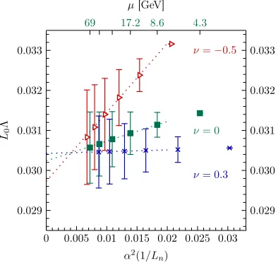
the second finite volume scheme, based on the gradient flow has paid off. The usually most problem-atic region of large couplings does not dominate the error as it did in the past. Observing the relatively large contribution to the error stemming from non-perturbative evolution of the SF coupling between 5 GeV and 70 GeV, the question arises whether one maybe could have used perturbation theory already at lower energies than we did. Fig.8shows theΛparameter in units ofL0, that one would obtain by
0 0.005 0.01 0.015 0.02 0.025 0.03 0.029
0.030 0.031 0.032 0.033
ν= 0
ν=−0.5
ν= 0.3
α2(1/Ln)
L0
Λ
69 17.2 8.6 4.3
0.029 0.030 0.031 0.032 0.033
µ[GeV]
Figure 8.Results forΛparameters in different SF schemes, depending on the energy from which on three-loop perturbation theory was used.
using the perturbative 3-loopβ-function starting from different energies. Purely perturbative behavior would show as a plateau in this plot. Although results starting fromα 0.14 are compatible with each other, we see a drift of the central value. This linear behavior ofL0Λas a function ofα2can be
explained by the presence of an effectiveb3 term in theβ-function. Relying on the 3-loop formula already atα ≈ 0.14 would reduce the statistical error significantly, but also introduce a systematic error of the order of 1σ.Such statements are highly scheme dependent. For instance Fig.8shows also
the situation for two slightly different SF-couplings – the truncation error can become much worse, or completely absent, depending on the chosen scheme. The family of SF schemes considered here is generally believed to be particularly well behaved perturbatively. In other schemes truncation er-ror could be much worse. An example is theαqq scheme. Although itsβ-function is known to four
loops, a significant deviation between perturbative and non-perturbative running can be observed at
αqq ≈0.24, [80].
For any future significant (e.g. factor 1/2 in the error) improvements of our programme several
challenging problems have to be overcome. The limited knowledge of boundary improvement coef-ficients will make pureO(a2) continuum extrapolations difficult. The subleading cutoffeffects in ¯g2
GF
will become significant and will have to be addressed, for instance by considering even finer lattices than the 164 → 324 ones used here. Electromagnetic and iso-spin effects in all quantities used for
![Figure 1. The left panel is PDG’s [1] summary of αS determinations. The yellow bands correspond to the pre-averages of different classes of determinations](https://thumb-us.123doks.com/thumbv2/123dok_us/8052420.1341738/2.482.51.409.80.258/figure-summary-determinations-correspond-averages-dierent-classes-determinations.webp)