Cryptanalytic Tradeoff Algorithms
Ga Won Lee and Jin Hong
Department of Mathematical Sciences Seoul National University, Seoul 151-747, Korea
{gwlee87,jinhong}@snu.ac.kr
June 22, 2014
Abstract
The performances of three major time memory tradeoff algorithms were com-pared in a recent paper. The algorithms considered there were the classical Hell-man tradeoff and the non-perfect table versions of the distinguished point method and the rainbow table method. This paper adds the perfect table versions of the distinguished point method and the rainbow table method to the list, so that all the major tradeoff algorithms may now be compared against each other.
Even though there are existing claims as to the superiority of one tradeoff al-gorithm over another alal-gorithm, the alal-gorithm performance comparisons provided by the current work and the recent preceding paper are of more practical value. Comparisons that take both the cost of pre-computation and the efficiency of the online phase into account, at parameters that achieve a common success rate, can now be carried out with ease. Comparisons can be based on the expected execu-tion complexities rather than the worst case complexities, and details such as the effects of false alarms and various storage optimization techniques need no longer be ignored.
A significant portion of this paper is allocated to accurately analyzing the exe-cution behavior of the perfect table distinguished point method. In particular, we obtain a closed-form formula for the average length of chains associated with a perfect distinguished point table.
Keywords: time memory tradeoff, distinguished point, rainbow table, perfect ta-ble, algorithm complexity
1
Introduction
A cryptanalytic time memory tradeoff algorithm is a method for inverting one-way functions with the help of pre-computed data. It is widely used today by hackers and also during criminal investigations to recover passwords from the knowledge of the password hash. In the pre-computation phase, massive amount of computations
specific to the one-way function of interest is performed and a compact digest of the obtained information is stored as tables. When the target image for inversion is given, further computations that utilize the pre-computed tables is performed to recover the pre-image with some probability, and this part is referred to as the online phase.
The execution behavior of any tradeoff algorithm can be manipulated through its many parameters. Existing analyses show that most tradeoff algorithms satisfy the tradeoff curve
T M2=cN2, (1)
for some small constant c, where T is the online execution time, M is the size of the memory space required to store the pre-computation tables, andNis the size of the space the one-way function is acting on. This means that if a tradeoff algorithm executes in timeT using tables of combined sizeMunder some set of its parameters, then given any otherT0 andM0 such that T M2=T0M02, there exists another set of parameters under which the algorithm will execute in timeT0using storageM0. Thus, each algorithm allows tradeoffs to be made between the online execution time and the storage requirement.
There are many time memory tradeoff algorithms available today, with most of them having roots in the classical algorithm by Hellman [7]. The most widely known algorithms are the distinguished point variant of the Hellman’s original algorithm [4,5] and the rainbow table method [12], which we shall refer to in this paper as the DP tradeoff and the rainbow tradeoff, respectively. Both of these algorithms have two subversions that work with the non-perfect tables and the perfect tables.
Comparison of tradeoff algorithm performances has been a controversial subject, with every newly announced algorithm claiming superiority over existing algorithms. The difficulty in accurately analyzing the execution behavior of these algorithms is clearly one reason for this confusion, but another source has been the absence of an acceptable method for numerically presenting the performances of tradeoff algorithms in a manner that closely reflects our intuition concerning their relative usefulness or practicality.
Let us take a moment to explain a reasonable method of tradeoff algorithm compar-ison that was recently suggested by [11]. Notice that the tradeoff curve (1) correspond-ing to any specific tradeoff algorithm presents the complete list of(T,M)-pair options that are made available by the algorithm. Thus the tradeoff curve expresses the required online resources or the online execution behavior of an algorithm completely, and one may accept thetradeoff coefficient c= T M2
N2 as a good measure of how efficiency an
algorithm is, with a smaller coefficient indicating a more efficient algorithm. Indeed, many previous claims as to the superiority of one algorithm over another have focused on this value.
In short, the online efficiency of each algorithm can be expressed succinctly through the tradeoff coefficient, but each algorithm allows further tradeoffs to be performed between the online efficiency, pre-computation effort, and success rate, while what we intuitively feel as the practicality or usefulness of an algorithm is directly connected to the overall behavior of the algorithm concerning these upper level tradeoffs. The difficulty of algorithm comparison lies in that, unlike the tradeoffs between time and storage that may commonly be expressed in the form (1) for most tradeoff algorithms, the equations that express the tradeoffs between the three aforementioned factors are very different among the major tradeoff algorithms. Hence, no single numeric value that can be computed for all algorithms in a common manner is likely to capture the performances of the algorithms concerning the upper level tradeoffs.
The solution suggested by [11] is to let the algorithm implementers make the final judgement and choice based on their requirements, available pre-computation and on-line resources, and personal taste, and to only present the information necessary for this decision in a coherent manner. Parameters for different algorithms are first restricted to those that achieve the same success rate. Then the tradeoffs between pre-computation cost and tradeoff coefficient are presented as curves for each algorithm. Each curve represents the complete list of options provided by one algorithm as to what degree of online efficiency can be obtained after a certain amount of pre-computation invest-ment, at the specified success rate. Implementers that place different relative values on the online efficiency and the pre-computation cost will choose to use different al-gorithms. In fact, comparisons of the algorithms themselves are no longer meaningful, and each implementer will choose an algorithm together with the online efficiency and pre-computation cost pair made available by that algorithm, based on his or her favored balance between the two factors, from among all the options made available by all the algorithms.
The work [11] first computes the success rates, pre-computation costs, and accu-rate tradeoff coefficients for the classical Hellman, non-perfect DP, and non-perfect rainbow tradeoffs. These complexities and properties are presented as functions of the algorithm parameters. Then, after fixing a small number of specific success rates of interest, parameters are restricted to those achieving these success rates, and the upper level tradeoffs between the pre-computation cost and tradeoff coefficient are presented as curves, separately for each algorithm. After carefully adjusting the units expressing the tradeoff coefficients for the three algorithms into one directly comparable unit, the three curves were superimposed into one graph. This comprehensive and coherent dis-play of information allows for someone considering the use of the tradeoff algorithms to decide on the most desirable balance between pre-computation investment and on-line efficiency from among the numerous options made available by the three tradeoff algorithms, at any required success rate.
preferred over the other four algorithms that have been mentioned. However, as we have discussed, the final judgement is not ours to make, and may be different under each specific situation.
Since this work is a direct extension of the work [11], we shall not repeat the con-tents of [11] that advocate the subject of our study. The readers are strongly urged to have at least a rough understanding of [11] before reading the current paper. In fact, it should be possible for the impatient reader with a full understanding of [11] to jump straight to Figure 3 and understand the core findings of this paper.
The rest of this paper is organized as follows. In the next section, we fix the ter-minology, clarify the exact versions of the algorithms we are analyzing, and review existing analyses of the perfect DP and perfect rainbow tradeoffs. Section 3 is devoted to fully analyzing the execution behavior of the perfect DP tradeoff, and is the most technical part of this paper. Analysis of the expected online time complexity that does not ignore false alarms is given and the tradeoff coefficient is computed. The issue of storage optimization is also discussed and tests that give strength to the correctness of our theoretical developments are presented. The perfect rainbow tradeoff is treated in Section 4. There are previous analyses we can utilize and obtaining the tradeoff coefficient for the perfect rainbow tradeoff is much easier than with the perfect DP tradeoff. The information we have prepared concerning the perfect DP and perfect rainbow tradeoffs is presented in Section 5 as graphs that allow direct comparisons between different algorithms and also between different parameter sets for the same al-gorithm. Finally, the paper is summarized in Section 6. The appendices contain further discussions that could be of interest. In particular, we explain in Appendix C that the existing analyses of the perfect DP tradeoff were not accurate enough for the purpose of algorithm comparisons.
2
Preliminaries
In this section, after setting the grounds of our discussion, we review some of the existing related works. Only the theoretical developments concerning the accurate time and storage analyses of the perfect DP and the perfect rainbow tradeoffs are explained. Some of the contents we do not present would include other tradeoff al-gorithms and implementation issues. There are also theories concerning asymptotic complexity bounds [2] on a general class of tradeoff algorithms and analyses of the full costs [17] of many cryptographic attack algorithms. We acknowledge that even the papers we introduce contain much more content than what is explained here.
The reader is assumed to be familiar with the basics of the tradeoff technique. In particular, the explicit tradeoff algorithms will not be explained. If the reader wishes for a quick overview of the tradeoff techniques that includes brief descriptions of the classical Hellman, distinguished point, and rainbow tradeoff algorithms, it will be con-venient to refer to [11], since the notation used here is compatible with that of [11]. The paper also clarifies many obscure technical details1that are not discussed elsewhere in
1Let us mention just one example. The objective of any tradeoff algorithm discussed in this work will be
to recover the randomly chosen exact input that was used to create the given inversion target, rather than to
the related literature, and which should be of interest to the mathematically oriented cryptographers.
2.1
Terminology, Notation, and Algorithm Clarification
Throughout this paper, the functionF:N →N will always act on a setN of sizeN
and thek-times iterated compositionF◦ · · · ◦F of function F is written as Fk. In practical applications, the functionF is the specific one-way function to be inverted, but it is treated as a random function during any theoretical analysis.
To reduce confusion, in this work, the wordefficiencyis always associated with an algorithm’s competitiveness in the use of the online resources, whereas the ability to balance the online efficiency, the pre-computation cost, and sometimes also the success rate, against each other, is referred to with the wordperformance.
The approximation(1−1
b)a≈e
−a
b, which is valid whena=O(b), is used fre-quently throughout this paper without any explanation. A more precise statement of this approximation may be found in [11, Appendix A]. Infinite sums are also frequently approximated by appropriate definite integrals throughout this paper. Both kinds of ap-proximations will be very accurate whenever we use them, as long as a reasonable set of parameters is used with the tradeoff algorithm, and will be written as equalities rather than as approximations.
Many parameters need to be fixed before any tradeoff algorithm can be put to use. Some of these are the chain lengtht, the number of rows or chainsmfor each pre-computation table, and the number of tables`. When working with the DP tradeoff, we assume a distinguishing property which is satisfied by a random point of the search spaceN with probability 1t, so that the expected length of a random DP chain ist. When dealing with perfect tables,mwill denote the number of distinct ending points or the number of rows after removal of merging chains, rather than the number of all chains that were initially generated while preparing the pre-computation table.
In the DP tradeoff case, the parameters are usually chosen so that mt2≈Nand `≈t. In the rainbow tradeoff case, it is more usual to havemt≈Nand a small number of tables`. We use notation ¯Dmsc=mt
2
N for the perfect DP tradeoff and ¯Rmsc=
mt
N for
the perfect rainbow tradeoff and refer to these values, which are assumed to be neither large nor very close to zero, as the matrix stopping constants. The corresponding value is written asDmscfor the non-perfect DP tradeoff.
We distinguish between a pre-computationtable, which consists of starting point and ending point pairs, and a pre-computationmatrix, which is the collection of all chains associated with a pre-computation table.
The coverage rate ¯Dcr of a perfect DP matrix is defined to be the expected
num-ber|DM¯ |of distinct nodes in a perfect DP matrix, divided bymt. More precisely, only the points that are used as inputs to the one-way function are counted, so that the ending point DPs are excluded in the count|DM¯ |and ¯DcrmtN is the success probability associated
with a single perfect DP table. The coverage rate ¯Rcr=| ¯
RM|
mt of a perfect rainbow matrix
is defined in exactly the same way.
Since there are many variations to the DP tradeoff, let us clarify the exact version of the DP tradeoff that will be analyzed in this work.
• The perfect table case is treated. If chain merges are discovered while computing a DP matrix, all chains except for the longest one among any set of merging chains are discarded [4, 5].
• Any implementation of the DP tradeoff will introduce an upper bound ˆton the length of pre-computation and online chains to deal with chains falling into loops [4, 5]. A lower bound ˇt can also be used [13, 16] to discard short pre-computation chains that contribute little to the search space coverage. In this work, no lower bound and a sufficiently large upper bound on chain lengths are assumed. This simplifies our theoretical developments by ensuring that the pos-sibility of an online chain not meeting the chain length bound conditions will be negligible, and also by allowing us to ignore the effects of discarding long or short pre-computation chains. A brief justification as to why treating just this case is sufficient is given in Appendix A.
• The work [4, 5] suggests that the chain lengths of each pre-computation chain and the maximum pre-computation chain length for each table be recorded in the DP table. However, the recording of individual chain lengths has a negative effect on the physical amount of required storage, and we can argue heuristically that the positive effect of the maximal chain length information is very limited. Neither suggestion is followed in this work.
• Sequential starting points, rather than random ones, are used [1, 3, 4]. Then, if
m0chains were generated per table before removal of merges, each starting point
can be recorded in logm0bits, which should be much smaller than the logNbits
required to record a random point.
• Knowledge of the distinguishing property makes certain parts of the ending point redundant. These parts are not recorded in the pre-computation table to save logt
bits of storage per ending point [3].
• The ending points are truncated to a certain length before being written to stor-age [2, 3]. Since some ending point information is lost, this will increase the frequency of false alarms. However, the side effects of truncation can be main-tained at a manageable level by controlling the degree of truncation. Details are discussed later in this work.
• The index file technique [3] is used in recording the pre-computation tables. This allows reduction of nearly logmfurther bits of storage per truncated ending point without any loss of ending point information.
stop the pre-computation chain regeneration at the exact position of chain merge, rather than at the common terminal DP.
• The work [8, 15] suggests that all the pre-computation tables be processed in parallel, rather than sequentially, during the online phase. For the case of non-perfect DP tradeoff, this idea was shown to have a small positive effect [10]. However, the parallel version of the perfect DP tradeoff will not be analyzed in this work. Treatment of parallelization is outside the scope of this work, but we expect our work to become an important stepping stone for anyone interested in analyzing the parallel version. Some comments on this issue are given in Appendix A.
There are also possible variations to the rainbow tradeoff, and the version treated in this work is clarified below. All techniques that we mention below are analogs of techniques we have already described for the DP tradeoff.
• The perfect table case is treated. Only one chain among any set of merging chains is retained [12]. All chains are of identical length and the method of choosing which chain to retain is irrelevant to our analysis and algorithm performance.
• Sequential starting points, rather than random ones, are used to reduce the stor-age requirements of the starting points.
• The ending points are truncated to an appropriate length, to be discussed later, before being written to storage.
• The index file technique is used to reduce logmfurther bits of storage per ending point.
• The small number of multiple rainbow tables are processed in parallel [12] dur-ing the online phase. This is not necessarily what is usually meant by the paral-lelization of an algorithm, in which case even the processing of each table would be shared by multiple processors. If the online phase must run on a single pro-cessor, the multiple tables can be processed in a round-robin fashion to simulate the parallel table processing.
Applications of the perfect table technique to the DP and rainbow tradeoffs are expected to increase both the online efficiency and the pre-computation cost. Hence, it is not clear if the benefit of using perfect tables outweighs its drawback. Providing information that can be used to settle this question is one of the objectives of this paper. Truncation of ending points must also be used carefully, since the storage reduction is associated with an increase in online time. However, all other techniques we are employing are only advantageous, when used appropriately in typical environments.
2.2
Existing Analyses of the Perfect DP Tradeoff
of the DP matrix into account was given by [4, 5]. There, credit is given to the unpub-lished work [13] for also having studied the DP tradeoff independently.
Many interesting variables were introduced by [4, 5] while analyzing the perfect DP tradeoff. The first of these is the expected number of chainsα after removal of merging chains. The average of DP chain lengthsβ0and ¯β, before and after removal
of merging chains, respectively, were also introduced. ( [4, 5] writes ¯β as β.) Note that the variableα is equal to the parametermused in this paper, but the work [4, 5] treated the number of pre-computation chains to be computed before collision removal as a given preset parameter and treatedα as a function of the initial chain count. The
success probability and online time estimates for the perfect DP tradeoff were given as equations involvingα and ¯β. They also stated certain relations satisfied byα,β0,
¯
β, and some other variables. However, they were unable to derive formulas for
com-putingαand ¯β from the externally provided parameters. Furthermore, as was pointed
out by [16], some of their arguments treated the merges of pre-computation chains inadequately and were problematic.
The subsequent work [16] gave a more advanced analysis of the perfect DP tradeoff. They started by computingβ0 for the case when the chain length bounds ˇt and ˆt are
both enforced. ( [16] writesβ0 as β.) Then the number of distinct nodes expected
in a perfect DP matrix was expressed using the variableβ0. Because ˇt and ˆt were
taken into consideration while computing the node count, the number of DP chains of any specified length range appearing in a perfect DP matrix could be extracted from the node counts by focusing on sub-matrices of the total DP matrix. The obtained information on the chain length distribution was then used in an ad hoc manner to compute ¯β. ( [16] writes ¯β asβmod.) Finally, the distinct ending point countα was
easily expressed as a function of the perfect matrix node count and ¯β.
Note thatα and the node count for a perfect DP matrix are directly connected to
the storage complexity and the success rate of the tradeoff algorithm, respectively. The paper also provides a simple argument concerning the pre-computation cost and an upper bound on the time complexity of the online phase.
The analysis of the perfect DP tradeoff given by [16] may seem rather complete, except that the effects of false alarms were disregarded during the time complexity analysis. Since we are also claiming to have done the same analysis, a comparison of results is given in Appendix C. Our observation is that the results of [16] are only valid as first approximations, and that these are too rough for the purpose of this paper.
The later work [1] also discussed the perfect DP tradeoff, but they only considered the special case when the DP matrix consists of the maximum number of non-merging DP chains that may be collected for a specified DP probability. However, during their analysis, they oddly assumed that the starting points for these chains are DPs. In any case, their result concerning the success probability requires knowledge of the average chain length associated with the maximal perfect DP matrix, but they were unable to provide this value except through experiments. Furthermore, since increasing the number of non-merging rows reduces the average chain length and possibly even the search space coverage, it is unclear if maximal perfect DP tables can be associated with being optimal in any sense.
( [14] writesβ0asβ.) The formulas of [14] and [16] forβ0will exhibit noticeable
dif-ferences only when ˆtis close toN, which is unrealistically large. After reobtainingβ0,
they derived a formula forαthat depends onβ0, but the argument was very terse and
their logics were not clear. Finally, the two variablesαandβ0were combined to give
the success probability of the tradeoff algorithm, but they seem to have confused the concepts ofβ0and ¯β at this point.
2.3
Existing Analyses of the Perfect Rainbow Tradeoff
The introduction of the rainbow tradeoff [12] was accompanied with a rudimentary analysis, which included the worst case online time complexity. The worst case refers to when the online phase algorithm processes all the pre-computation tables without returning the correct answer. However, the effects of false alarms were not accounted for in this worst case complexity claim. They compared the worst case complexity against the similarly rough worst case complexity of the DP tradeoff and claimed that the rainbow tradeoff was more efficient by a factor of two. This was then combined with heuristic arguments, mainly concerning false alarms, for a claim in much higher advantage. Most of their arguments referred to the non-perfect rainbow tradeoff and the perfect table version made an appearance only at the end of the paper, but the complexity analyses provided were rough enough to be applicable to both versions.
A more serious analysis of the perfect rainbow tradeoff appeared in [1]. It treated the expected online time complexity, rather than the worst case complexity, and took the effects of false alarms into account. Their stated complexity results hold true only in the case of maximal perfect tables, but a large part of these results and their proofs can be adjusted to hold true for the general perfect rainbow tables.
The expected online time complexity of the perfect rainbow tradeoff that does not ignore false alarms was also given by [9]. There the complexity results for the general perfect rainbow tables were stated as closed-form formulas. These are easier to use and manipulate than the formulas of [1], which were given as certain double summations that further involved iterative computations if the general perfect rainbow tables were to be considered. However, the results of [1] and [9] should agree accurately when numerically evaluated on any specific set of reasonable parameters.2 Our theoretical developments concerning the perfect rainbow tradeoff will rely heavily on these results. Concerning the success rate of the rainbow tradeoff, note that this is trivial to write down for the perfect table version [12]. A formula for the success rate of even the non-perfect rainbow tradeoff already appeared in [12]. However, iterative computations were required to evaluate the formula on any specific parameter set. A simple closed-form closed-formula that can replace this iterative part, for the special case ofNstarting points, was presented in [1], while studying the success rate of the maximal perfect rainbow tradeoff. The closed-form formula was slightly modified in [9] to work for any non-perfect rainbow table and was used to study the online complexities of the rainbow tradeoff. The success rate of the non-perfect rainbow tradeoff is not used directly in this work, but plays a crucial role in studying the behavior of false alarms in the perfect
2The analyses of [1] and [9] extend further to the application of checkpoints [1] on the perfect rainbow
rainbow tradeoff, and the current work relies on previous results [1,9] that have worked out these details.
Let us mention one more issue that is not necessarily specific to the perfect rainbow tradeoff, but is closely related to this work. The work [2] claimed that each entry in the pre-computation table for the DP tradeoff can be represented by half the number of bits required for the rainbow tradeoff, but their explanation was rather brief. They followed this claim with a short argument stating that, if the effects of false alarms were to be ignored, one must conclude that the DP tradeoff is twice as efficient as the rainbow tradeoff. An attempt to refute this was made by [1], which maintained that the claim of [2] concerning the required storage bits per table entry was incorrect. With neither [2] nor [1] providing any detail, the work [11] clarified that, in the case of non-perfect tradeoffs, the storage requirement comparison of [2] was correct, but that the rainbow tradeoff may still be seen as being advantageous over the DP tradeoff in typical environments. However, the case of the perfect tradeoffs was left untreated.
3
Perfect DP Tradeoff
In this section, we deal with the perfect DP tradeoff that uses a sufficiently large upper bound and no lower bound on the chain length. Before starting our main analysis, let us check how often one can expect to see over-length chains when using a sufficiently large chain length bound.
The probability for a chain generated from a given starting point to fall into an infinite loop without reaching a DP within its first ˆtiterations is
1
N+
1−1 t −
1
N
2
N+
1−1 t −
1
N
1−1 t −
2
N
3
N+· · · ·
· · · ·+1−1 t −
1
N
1−1 t −
2
N
· · ·1−1 t −
ˆ
t−2
N
tˆ−1
N ,
(2)
and the probability for a chain not to reach a DP within its first ˆt iterations, without falling into a loop, is
1−1 t −
1
N
1−1 t −
2
N
· · ·1−1 t −
ˆ
t−2
N
1−1 t −
ˆ
t−1
N
. (3)
The sum of these two terms is the probability for a chain not to reach a DP within its first ˆtiterations, and may be approximated by
1
N+
1−1 t
2
N+· · ·+
1−1 t
ˆt−2tˆ−1
N +
1−1 t
ˆt−1
, (4)
under the conditionttˆN. If we further assume that ˆtt is not too large, we may approximate the above once more with
t2 N
Z tˆ
t
0
e−uu du+e−ttˆ=t 2
N
n
1−1+tˆ
t
e−ttˆ o
This probability approaches tN2 =O m1very quickly, as ttˆ is increased. For ex-ample, even at the moderately large chain length bound of ˆt=15t, the probability for a randomly generated chain to be discarded due to its length is tN20.999995+3.05902
107 ,
which is small enough for our purposes. However, because of the first term, which cor-responds to looping chains, the number of long chains expected during the generation of a full DP matrix cannot be made arbitrarily close to zero by increasing the chain length bound.
3.1
Online Efficiency
This is the most complicated part of this paper. We will present formulas describing the success probability, pre-computation cost, and tradeoff coefficient of the perfect DP tradeoff.3 The discussion will require previous results concerning the non-perfect DP tradeoff.
Let us visualize a non-perfect DP matrix as having been aligned at the ending points and usem←k to denote the number of distinct points expected in its column that isk
iterations away from the ending points. In particular,m←0denotes the number of
non-merging rows in the DP matrix.
Lemma 1. We havem←0≈
←
m1. In other words, in a non-perfect DP matrix, the number
of distinct ending points may be approximated by the number of distinct points that are a single iteration away from these ending point DPs.
Proof. Given a set ofm←1points, which are known to be a singleF-iteration away from
the DPs, the size of itsF-image is expected to be ←
m0= (N/t) n
1−1− 1 N/t
m←1o
= (N/t)n1−1+
← m1t
N −
←
m1
2
t N
2 +· · ·o
=m←1+O
(m←1)2t
N
=m←1
n
1+O1 t
o
.
Thus, we may approximatem←0with
←
m1, unlesstis very small.
More generally, it is possible to showm←i+1≈
←
mi, but it would be unwise to
itera-tively combine these approximations too many times to concludem←j≈
←
mi, for every j
andi. In fact, it is easy to argue as in [10] that ←
mk=|DM|
1−1 t
k−11
t, (6)
fork≥1, so thatm←j = 1−1tj
−i←
mi. Here, the|DM|denotes the number of distinct
points expected in a non-perfect DP matrix. To be more precise, the|DM|used here counts the points that were used as inputs to the iterating function during the non-perfect DP table creation, so that the starting points are included and the ending points are excluded.
3We thank Wenhao Wang of IIE CAS for bringing an error that was contained in a previous version of
In passing, we caution the reader that one must be aware of the possibility of erring when extending (6) to thek=0 case and writing
← m0=|DM|
1−1 t
−11
t ≈ |DM|
1
t
1+1
t
, (problematic!) (7)
since one can infer from the proof of Lemma 1 that the correct value is closer to
← m0≈
← m1
n
1−( ← m1−1)t
2N
o
≈ |DM|1 t
1−D¯msc 2t
. (8)
These two expressions form←0are certainly close to each other and also to
←
m1, so that the
use of (7) could be acceptable under many circumstances, but it would be inappropriate to claim (7) by itself.
The core information missing from (6) is also already available. It is known [11] that a single non-perfect DP matrix created withm0starting points is expected to
con-tain
|DM|= 2m0t 1+√1+2Dmsc
(9)
distinct points, whereDmsc=m0t
2
N is the matrix stopping constant for the non-perfect
DP matrix. The information we have gathered so far can be used to related the number of starting points to the number of distinct ending points.
Lemma 2. A non-perfect DP matrix created with m0 starting points is expected to
contain 2m0
1+√1+2Dmsc non-merging chains, whereDmsc=
m0t2
N . Conversely, to create a perfect DP matrix containing m non-merging chains, one must expect to generate m0= 1+D¯msc2
m chains.
Proof. Lemma 1 and (6) together imply that |DM|t is the number of non-merging chains. Hence, the first claim follows from (9).
As for the second claim, it suffices to solve form0in
m=|DM|
t =
2m0
1+p1+2m0t2/N
.
After rewriting this in the form
1+ r
1+2 ¯Dmsc
m0
m =2 m0
m,
one can solve form0
m, so as to expressm0as a function of ¯Dmscmultiplied bym.
Note that the first sentence of this lemma gives a simple formula for the number of non-merging chainsα, discussed in Section 2.2, which many previous works had
attempted to find.
For the remainder of this section,
m0=
1+D¯msc 2
will always denote the number of starting points that are required to create a perfect DP table containingmnon-merging chains. This equation is equivalent to
Dmsc=
1+D¯msc 2
¯
Dmsc, (11)
and again to
¯
Dmsc=
p
1+2Dmsc−1, (12)
which can be used to convert any formula given in terms of ¯Dmscinto one given in terms
ofDmsc.
Another interesting formula that follows from the notational convention (10) is
|DM|=mt, (13)
which is evident from the first equation in the proof to Lemma 2. That is, the non-perfect DP matrix created fromm0 starting points, as given by (10), is expected to
covermtdistinct points.
The pre-computation phase of a perfect DP tradeoff requiresm0t`iterations of the
one-way function. We define thepre-computation coefficientfor the perfect DP trade-off to be ¯Dpc=mN0t`, so that the cost of pre-computation is ¯DpcN. The following
state-ment is a direct consequence of Lemma 2.
Proposition 3. The pre-computation coefficient of the perfect DP tradeoff is
¯
Dpc=
1+D¯msc 2
mt`
N .
By the definition of the coverage rate, the success probability of the perfect DP tradeoff may be stated as
¯
Dps=1−
1−mtD¯cr N
`
=1−exp−mt`
N D¯cr
, (14)
and we can combine this with Proposition 3 to claim the following.
Proposition 4. The success probability of the perfect DP tradeoff is
¯
Dps=1−exp
−2 ¯DpcD¯cr 2+D¯msc
.
We have succeeded in obtaining expressions for ¯Dpcand ¯Dpsthat do not involvem0.
Our next short term objective is to obtain such an expression for ¯Dcr. Some technical
lemmas need to be prepared first.
Given a functionF:N →N and a nonnegative integerk, we defineDk(F)orDk
to be the set of elements ofN that arek-manyF-iterations away from their closest DPs. In particular,D0is the set of DPs. It is clear that{Dk(F)}∞k=0is a partition ofN,
and that we can expect the sizes of these subsets to be
|Dk|=N
1−1 t
k1
t, (15)
Lemma 5. Let F:N →N be chosen uniformly at random from the set of all functions acting onN and let us fix a set D⊂Dk(F)for some k≥1. Then the expect sizes of its
iterated images under F will satisfy |Fi(D)| N(1−1
t)k
−i1
t
= 1−exp − |F
i−1(D)|
N(1−1
t)k
−i1
t
!
,
for each i=1, . . . ,k.
Proof. For a random functionF:A →Bdefined on finite sets and a subsetC of the domainA, the image size is expected to be
|F(C)|=|B|n1−1− 1 |B|
|C|o
=|B|n1−exp−|C|
|B|
o
.
The claim is now a direct consequence of the set sizes given by (15). A more detailed proof is provided in Appendix B, for those interested in the subtleties hidden behind this short argument.
It is possible to work out the iterations expressed by this lemma and write down each iterated image size as a closed-form formula.
Lemma 6. Let F:N →N be a random function and let D⊂Dk(F), for some k≥0.
When|D|=O(m), the size of the i-th iterated image under F is expected to be |Fi(D)|= 2|D|
2+D¯msc
|D|
m e
k
t(1−e−ti) ,
for each0≤i≤k.
Proof. Let us temporarily introduce the notation fi=
|Fi(D)|
N(1−1
t)k−i
1
t
, and rewrite Lemma 5 as
fi=1−exp
n
−1−1 t
fi−1 o
=1−1
t
fi−1−
1 2
1−1 t
2
fi2−1+· · ·. The condition|D|=O(m)implies fi=O 1t
so that we can state
fi−fi−1=−
1
t fi−1−
1 2f
2
i−1+O
f2
i−1
t
.
Noting that f
2
i−1
t is of strictly smaller order than fi−1
t + fi2−1
2 , one solves the
correspond-ing differential equation
f0(x) =−1 t f(x)−
1 2 f(x)
2
with the initial condition f(0) =f0=
|D|t
Ne−kt
, to obtain
fi=
2|D|t
2Nei−tk+ (e i
t−1)|D|t2 ,
The previous two lemmas were prepared to support the next lemma, which gives the probability for a single chain to merge into a set of chains. This information will be used to study the inner workings of how a perfect DP table is formed from a non-perfect DP table.
Lemma 7. Let F:N →N be a random function and let D⊂Dk(F), for some k. When|D|=O(m), the probability for a random point x∈Dk(F)to satisfy Fk(x)6∈
Fk(D)is
n
1+D¯msc 2
|D| m e
k
t −1
o−2
.
Proof. The probability in question is given by
k
∏
i=0
1−|F
i(D)|
|Dk−i|
=
k
∏
i=0
1− |F
i(D)|
N(1−1
t)k
−i1
t
=1− |D|t
Ne−kt
k
∏
i=1
1− |F
i(D)|
N(1−1
t)k
−i1
t
.
By applying Lemma 5 to the product ofkterms, we can write
k
∏
i=1
1− |F
i(D)|
N(1−1
t)k
−i1
t
=
k
∏
i=1
exp− |F
i−1(D)|
N(1−1
t)k
−i1
t
=exp −1−1
t
k−1
∑
i=0
|Fi(D)|
N(1−1
t)k−i
1
t
!
.
Since we are given the condition |D|=O(m), we can apply Lemma 6, or the last equation in its proof, and compute the sum inside the exponential function as
k−1
∑
i=0
|Fi(D)| N 1−1
t
k−i1
t
=
k−1
∑
i=0
2|D|t
2Nei−tk+ (eti−1)|D|t2 =
Z k/t
0
2|D|t
2N
t e
−k
teu+ (eu−1)|D|t
du=2 lnn1+|D|t 2
2N e
k
t −1
o
.
By substituting the sum back into the exponential function, we get
k
∏
i=0
1−|F
i(D)|
|Dk−i|
=1− |D|t
Ne−kt n
1+D¯msc 2
|D| m e
k
t −1
o−2(1−1t)
.
The(1−1
t)term in the exponent is insignificant and the condition|D|=O(m)allows
us to ignore the first product term. Hence, we arrive at the claimed formula.
With the help of the technical lemmas that have been prepared, we can finally present something of more direct practical value.
Proposition 8. The coverage rate of a perfect DP matrix is
¯
Dcr=
2 ¯
Dmsc
ln1+D¯msc 2
Proof. Consider a pre-computed non-perfect DP matrix and the process of removing chains to obtain a perfect DP matrix. A chain survives through the collision removal process if and only if it does not collide with another chain that is longer than (or equal to) its length. Hence, according to Lemma 7, the probability for a chain of lengthkin a non-perfect DP table to remain in the perfect table is
n
1+D¯msc 2
← mk
m e
k
t −1
o−2
.
This figure is a slight underestimate since the collisions among chains of the same length were reflected too many times, but such collisions are rare and will not cause noticeable inaccuracy.
Since the number of, possibly merging, chains of lengthkism0 1−1t
k−1 1
t and
the perfect table contains no overlapping of points, the number of distinct points in the perfect DP table is
∞
∑
k=1
k·m0
1−1 t
k−11
t ·
n
1+D¯msc 2
← mk
m e
k
t −1
o−2
.
This formula does not count the ending points and only includes the points that were used as inputs to the iterating function during the DP table computation.
The coverage rate of the perfect DP matrix is given by
¯
Dcr=
1
mtm0
1−1 t
−1 ∞
∑
k=1
k t ·e
−k t ·
n
1+D¯msc 2 e
−k t
1−1 t
−1
ekt −1
o−2
,
where we have used (6) and (13) to remove them←kterm. After ignoring the insignificant
(1−1
t)
−1terms, the coverage rate can be computed as
¯
Dcr=
m0
m
Z ∞
0
u e−un1+D¯msc 2 1−e
−uo−2
du=m0
m
ln 1+D¯msc
2
¯
Dmsc
2 1+
¯
Dmsc
2
.
It now suffices to recall Lemma 2 to arrive at the claimed formula.
Let us briefly digress and recall the average chain length ¯βof a perfect DP matrix,
introduced in Section 2.2. By definition, it is the number of points in a perfect DP matrix divided by the number of its ending points, and we can easily write it as
¯
β=|
¯ DM|
m = mtD¯cr
m =t
2 ¯
Dmsc
ln1+D¯msc 2
. (16)
Should it be required, we can use (12) to rewrite this in terms of the parametersm0
andtas
¯
β =t1+ √
1+2Dmsc
Dmsc
ln1+ √
1+2Dmsc
2
, (17)
whereDmsc= m0t
2
N . It is easy to check that this ¯β value is always smaller than the
keeping the longest of any set of merging chains, the longer chains are more likely to merge into one another and be discarded.
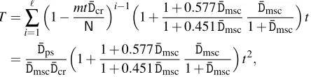
Unlike other results of this work, our next claim is mostly based on an experimental evidence, rather than on purely theoretical arguments. Recall that the processing of a perfect DP table can bring about at most one alarm, which requires the partial regen-eration of a single pre-computation chain. We will later show in Section 3.3 that, for a wide range of parametersmandt, which covers all parameter combinations of interest, the value computed through the formula
t×1+0.577 ¯Dmsc 1+0.451 ¯Dmsc
(18)
agrees accurately with the experimentally obtained average number of one-way func-tion iterafunc-tions required for this partial chain regenerafunc-tion.
Let us clarify that we are not claiming formula (18) to becorrectin any theoretical sense. In fact, we know that the very different formula
t1+0.340468n1−1.32798 ¯
Dmsc
ln1+ D¯msc 1.32798
o
(19)
works equally well for parameters of interest. Our only claim here is that formula (18) predicts the average cost of resolving each alarm with accuracy that is more than suffi-cient for most practical purposes.
Proposition 9. The processing of a single perfect DP table is expected to require t×1+0.577 ¯Dmsc
1+0.451 ¯Dmsc
¯
Dmsc
1+D¯msc
.
invocations of the one-way function in relation to the resolving of a possible alarm. Proof. As the work factor (18) is already available, it only remains to find the proba-bility of encountering an alarm.
An online chain will merge into a perfect pre-computation matrix ¯DMif and only if it merges into the corresponding non-perfect pre-computation matrixDM. Since (13) states the number of elements contained inDMasmt, the probability of merge can be stated as
∞
∑
i=0
1−1 t −
mt N
imt
N =
¯
Dmsc
1+D¯msc
.
The claimed expected cost of dealing with a possible alarm is the product of this prob-ability and the work factor (18).
Having obtained the cost of dealing with alarms, the online complexities of the perfect DP tradeoff can be expressed as a single tradeoff curve.
Theorem 10. The time memory tradeoff curve for the perfect DP tradeoff is T M2= ¯
DtcN2, where the tradeoff coefficient is given by
¯
Dtc=
1+1+0.577 ¯Dmsc 1+0.451 ¯Dmsc
¯
Dmsc
1+D¯msc
D¯psln(1−D¯ps) 2
¯ DmscD¯cr3
Proof. The probability for the i-th DP table to be processed during the online phase executed for a single inversion target is 1−mtD¯cr
N
i−1
. The online processing of each table is expected to requirest iterations of the one-way function for the online chain creation and the expected number of iterations required to deal with the alarms that could occur is given by Proposition 9. Hence, the number of one-way function itera-tions expected during the online phase is
T = `
∑
i=1
1−mtD¯cr N
i−1
1+1+0.577 ¯Dmsc 1+0.451 ¯Dmsc
¯
Dmsc
1+D¯msc
t
= D¯ps
¯ DmscD¯cr
1+1+0.577 ¯Dmsc 1+0.451 ¯Dmsc
¯
Dmsc
1+D¯msc
t2,
where the second equality relies on (14) or Proposition 4. The tradeoff curve is obtained by combining this time complexityT with the storage complexityM=m`as follows:
T M2= D¯ps ¯ DmscD¯cr
1+1+0.577 ¯Dmsc 1+0.451 ¯Dmsc
¯
Dmsc
1+D¯msc
(mt`)2
= D¯ps
¯ DmscD¯cr
1+1+0.577 ¯Dmsc 1+0.451 ¯Dmsc
¯
Dmsc
1+D¯msc
nln(1−D¯ps)
¯ Dcr
o2
N2.
Once again, Proposition 4 is required to obtain the second equality.
3.2
Storage Optimization
An analysis of the perfect DP tradeoff would not be complete without a discussion of the storage optimization techniques. Dealing with the storage size of the starting points is quite straightforward. One requires logm0 bits of space for every starting
point, and (10) implies that this will be one or two bits more than logmfor parameters of interest. Hence, one may safely claim that the number of bits required to store a single starting point for a perfect DP tradeoff is very close to that required for the non-perfect DP tradeoff, when comparable parameters are used by the two algorithms. To deal with the ending point storage, one needs to discuss the effects of truncating ending points before storage. Consider an ending point truncation method for which two random DPs, truncated in the specified manner, will have probability1r of matching with each other. We shall express such a situation as having a1r probability of truncated match. One specific way to do this would be to retain just logrbits of the ending point that are unrelated to the DP definition. Note that we are considering truncations of DPs only and not of the general points ofN .
The effects of ending point truncation on the perfect DP tradeoff is slightly different from that on the non-perfect DP tradeoff, which was treated in [11]. The truncation may cause two non-merging pre-computation chains to become indistinguishable at the ending points and cause more chains to be discarded. However, the following lemma shows that these further collisions can mostly be avoided by recording slightly more than logmbits.
r1−exp(−m
r) distinct truncated points. Conversely, when r>m, one must expect
to truncate rln r−rmDPs in order to collect m distinct truncated points.
This lemma is a trivial consequence of treating the truncation process as the random selection of points from a pool ofr-many points.
Let us consider a specific example. Whenr=25mis used for truncation, it suffices
to truncate 32mln 3231
=1.01596mDPs in order to obtainmdistinct truncated ending points. Combining this information with Proposition 3, one can state that, by recording just 5+logmbits of each ending point, one can control the extra pre-computation necessitated by the ending point truncation to within approximately 2%. Note that this is not 1.596% and only claimed approximately, because the variable mappears not only in the mtN` term of Proposition 3, but also inside the D¯msc
2 term. In any case, the
effects of ending point truncation on the collision of ending points can be maintained at an ignorable level by retaining a little more than logmbits of information through the truncation process. Note that by ignoring the ending point collisions induced by truncations, we are also ignoring their effects on the pre-computation time and also on the coverage rate, or, equivalently, the success probability.
We now need to discuss the effects of truncation on the online time. The terminating DP of the online chain must be searched for among the truncated ending points, so we have the possibility of falsely announcing a match and then regenerating the pre-computation chain to resolve this alarm.
Lemma 12. Assume the use of an ending point truncation method with a 1r probabil-ity of truncated match. Further assume that r has been chosen to be large enough so that the occurrences of indistinguishable ending points caused by truncations are suf-ficiently limited to be ignored. Then the number of extra one-way function invocations induced by truncation-related alarms is expected to be
tm r
2 ¯
Dmsc(1+D¯msc)
ln1+D¯msc 2
,
for each fully processed perfect DP table.
Proof. Let us compute the probability for an online chain to become a DP chain of lengthiand not merge into the perfect DP matrix, but have a truncated ending point that coincides with a truncated ending point in the perfect DP table. For this event to occur, the online chain must be created in the following manner: (1) Random choices for the firsti nodes of the online chain, starting from the correct pre-image of the inversion target, must be made among the DPs that do not belonging to the non-perfect DP matrix, which is seen before the removal of merging chains; (2) The final point is chosen among DPs that is different from themending points; (3) Furthermore, the final point must be chosen so that its truncation matches one of themtruncated ending points. The process (2) and (3) are not quite independent, but since the number of DPs is much greater than the number of points we know the final point not to be, i.e.,Nt m, the dependence can be ignored. Thus, the probability we seek is
1−1 t −
|DM| N
i1
t − m N
m
r ≈
1−1 t −
|DM| N
i1
t m
r =
1−1+D¯msc t
i1
t m
where we have used mN =O(mt1) =o(1t)for the approximation and (13) for the final equality. Thus, the probability for the online processing of a perfect DP table to cause a truncation-related alarm, i.e., an alarm that does not involve the online chain merging into the pre-computation matrix, is given by
∞
∑
i=1
1−1+D¯msc t
i1
t m
r =
1−1+D¯msc
t
1+D¯msc
t
1
t m
r ≈
1 1+D¯msc
m r.
Notice that the length of a pre-computation chain is independent of how likely it is to be involved in a truncation-related alarm. Hence, the number of iterations required to regenerated the pre-computation chain involved with such a pseudo-collision is ex-pected to be the average chain length of the perfect DP matrix, which is given by (16). The cost of resolving alarms that are induced by truncation is
1 1+D¯msc
m rt
2 ¯
Dmsc
ln1+D¯msc 2
,
for the full processing of a single perfect DP table.
The normal one-way function iterations required to generate the online chain and deal with a possible alarm while processing a single perfect DP table was stated during the proof of Theorem 10 to be
1+1+0.577 ¯Dmsc 1+0.451 ¯Dmsc
¯
Dmsc
1+D¯msc
t. (20)
If we assume that sufficient information is left after the ending point truncation so that the number of indistinguishable ending points are kept ignorably small, then, at the typ-ical parameter of ¯Dmsc=1, the expected numbers of normal iterations and
truncation-related iterations become (1+11..57745112)t=1.54342t and ln(32)mrt =0.405465mrt, re-spectively. For example, at logr=5+logm, the ending point truncation increases the number of one-way function iterations by a mere 0.405465
1 32t
1.54342t ≈0.82%. The following
can be stated for the general situation.
Proposition 13. Suppose that the online phase of a perfect DP tradeoff implementa-tion that stores each ending point in full requires T iteraimplementa-tions of the one-way funcimplementa-tion to complete. Consider the use of an ending point truncation method with a1r probability of truncated match, wherelogr=ε+logm. Ifεis large enough for the occurrences of indistinguishable ending points caused by truncations to be ignored, then the imple-mentation with the ending point truncation requires
2 ln 1+D¯msc
2
¯
Dmsc(1+D¯msc) 1+11++00..577 ¯451 ¯DDmscmsc 1+D¯mscD¯msc
T
2ε
additional iterations of the one-way function to complete.
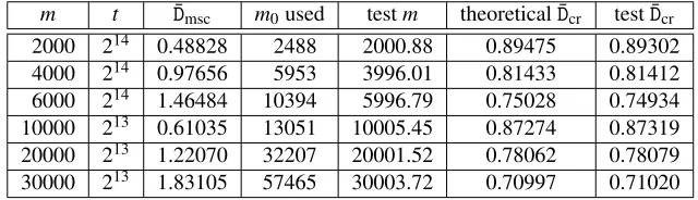
Table 1: The number of DP chains before and after removal of chain merges and the coverage rate of the perfect DP matrix. (N=240; ˆt=15t).
m t D¯msc m0used testm theoretical ¯Dcr test ¯Dcr
2000 214 0.48828 2488 2000.88 0.89475 0.89302
4000 214 0.97656 5953 3996.01 0.81433 0.81412
6000 214 1.46484 10394 5996.79 0.75028 0.74934
10000 213 0.61035 13051 10005.45 0.87274 0.87319
20000 213 1.22070 32207 20001.52 0.78062 0.78079
30000 213 1.83105 57465 30003.72 0.70997 0.71020
DPs can be truncated so that a little more than logmbits of information is retained with very little negative effect on the success probability, pre-computation cost, and online time. The index file technique can be used to remove almost logmfurther bits per ending point without any loss of information. In conclusion, storage of each starting point and ending point pair requires a little more than logmbits. This was also the conclusion obtained for the non-perfect DP tradeoff in [11].
3.3
Experimental Results
We have verified the correctness of major parts of our complexity analysis with experi-ments. For the first two sets of our experiments, the one-way function was instantiated with the key to ciphertext mapping, under a randomly fixed plaintext, of the block-cipher AES-128. Freshly generated random plaintexts were used to create different one-way functions that were required for repetitions of the same test. Bit-masking of ciphertexts to 40 bits and its zero-extension to 128-bit keys were used to restrict the search space to a manageable size ofN=240.
The first experiment was designed to verify Lemma 2 and Proposition 8 simulta-neously. Recall that Lemma 2 related the number of starting points to the number of non-merging chains in a DP matrix and that Proposition 8 presented the coverage rate of the perfect DP matrix.
After fixing suitable parametersmandt, we first computed them0value, as
spec-ified by (10). We generated chains fromm0distinct starting points and recorded their
terminating DPs, together with their respective chain lengths. A small number of chains that extended beyond the moderately large chain length bound of ˆt=15t were dis-carded during this process. After dealing with chain merges by retaining only the information corresponding to the longest chain among any set of merging chains, the number of remaining DPs were counted. Next, the lengths of the surviving chains were added together and taken as the number of distinct entries in the perfect DP matrix. The obtained count of matrix entries, divided bymt, is our test ¯Dcrvalue. The whole process
was repeated 200 times for each choice of parameter set and the obtained values were averaged.
The test results are summarized in Table 1, together with the integerm0values we
starting points is very close to the targetedmvalue, in spite of the small number of test repetitions. It can also be seen that our theory was able to predict the coverage rates accurately.
Even though this test gives some confidence as to the correctness of our theory, let us present another test that makes sure that our accurate predictions of the coverage rate did not result from some lucky averaging effect that conveniently hid logical errors in our lower level arguments.
Recall that the proof of Proposition 8 relied heavily on our ability to write the probability for a random chain of lengthknot to merge into any of the chains in a non-perfect DP matrix that are longer thank. More specifically, this probability was taken to be
n
1+D¯msc 2 1−e
−k
t
o−2
(21)
and was interpreted as the probability for a chain in a non-perfect DP matrix to survive through the process of removing chain merges.
To test this core logic, we first generated multiple non-perfect DP matrices, discard-ing the small number of chains reachdiscard-ing the length bound of ˆt=15t. Then, for each 1≤k<tˆ, we counted and recorded the total number of chains of lengthkfound among these matrices. Next, we removed merges from each of the DP matrices to create multi-ple perfect DP matrices and, once again, recorded the number of chains of each length. We took the ratio of the two chain counts, for each lengthk, as our test value of the probability for chains of lengthkto survive through the chain merge removal process. Note that this ratio of counts cannot be computed separately for each DP matrix and then later averaged over multiple DP matrices, since the number of chains of any given length is likely to be very small and often zero for any single DP matrix.
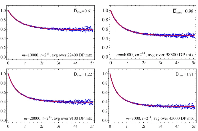
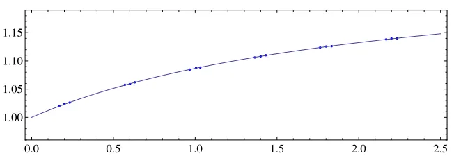
The test results are provided by Figure 1. The probability (y-axis) for chain survival through the chain merge removal process is given for each chain length (x-axis). The lines correspond to our theory, as given by (21), and the dots represent the count ratios obtained through tests. Even though our chain length bound was ˆt =15t, we have displayed the data only for chain lengths less than approximately 5t. Furthermore, in each box, we only plotted approximately 500 dots that are equally spaced in terms of chain length values, since densely packing all 5t dots into each box made the graphs harder to comprehend.
The experimental data agrees well with our theory in all the boxes. Notice that the test results are less reliable at the large chain lengths. This is because longer DP chains appear less frequently and these large chain length data were obtained from a smaller number of chains. A much larger number of DP matrices would need to be generated to obtain meaningful test values at lengths much larger than 5t.
••••••••••••••••••••••• ••••••••••••••••••
••••••••••••••••••••••••••••••••••••••••••••••••••••••••• ••••••••••••••••••••••••••••••••••••••••••••••••••••••••••••
•••••••••••••••••••••••••••••••••••••••••••••••••••••••••••••••••••••••••••••••••••••••••••••••••••••••••••••••••••••••••••••••••••••••••••••••••••••••••••••••••••••••••••••••••••••••••••••••••••••••••••••••••••••••••••••••••••••••••••••••••••••••••••••••••••••••••••••••••••••••••••••• • •••••••••••••
• • ••••• • ••••••••
•••••• ••••••
••••• •• ••••••••••••
Dmsc=0.61
m=10000,t=213, avg over 22400 DP mtx
0 t 2t 3t 4t 5t
0.0 0.2 0.4 0.6 0.8
1.0 •••••••
•••••••••••••••••••• ••••••••••••••
•••••••••••••••••••••••••••••••••••••••••••••••
••••••••••••••••••••••••••••••••••••••••••••••••••••••••••••••••••••••••••••••••••••••••••••••••••••••••••••••••••••••••••••••••••••••••••••••••••••••••••••••••••••••••••••••••••••••••
•••••••••••••••••••••••••••••••••••••••••••••••••••••••••••••••••••••••••••••••••••••••••••••••••••••••••••••••••••••••••••••••••••••••••••••••••••••••••••••• •••••••••••••••••••••••••••••••••••
• •••••••••••••••••••••••••••••••••••• Dmsc=0.98
m=4000,t=214, avg over 98300 DP mtx
0 t 2t 3t 4t 5t
0.0 0.2 0.4 0.6 0.8 1.0
••••••••••• ••••••
••••••••• ••••••••••••••••••••••••
••••••••••••••••••• •••••••••••••••••••••••••••••••••••••••••••••••••••••••••••••••••••••••
••••••••••••••••••••••••••••••••••••••••••••••••••••••••••••••••••••••••••••••••••••••••••••••••••••••••••••••••••••••••••••••••••••••••••••••••••••••••••••••• ••••••••••••••••••••••••••••••••••••••••••••••••••••••••••••••••••••••••••••••••••••••••••••••••••••••
• ••••••••••••••••••••••••••••••••••••••••••••••••••••••••
• ••••••••••••••••••
•• ••• • • •• •• • •• • •• •••••••••
••
Dmsc=1.22
m=20000,t=213, avg over 9100 DP mtx
0 t 2t 3t 4t 5t
0.0 0.2 0.4 0.6 0.8
1.0 •••
••••••• ••••••••••
••••••••••••••••• ••••••••••
••••••••••••••••••••••••••••••••••• •••••••••••••••••••••••••••••••••••••••••••••••••••••••••••••••••••••••••••••••••••••••••••••••••••••••••••••
••••••••••••••••••••••••••••••••••••••••••••••••••••••••••••••••••••••••••••••••••••••••••• ••••••••••••••••••••••••••••••••••••••••••••••••••••••••••••••••••••••••••••••••••••••••••••••••••••••••••••
••••••••••••••••••••••••••••••••• • ••••••••••••••••••••••
••••••••••••••••• • ••••••••••••••••••••
• ••••• • • ••••••••••
Dmsc=1.71
m=7000,t=214, avg over 45000 DP mtx
0 t 2t 3t 4t 5t
0.0 0.2 0.4 0.6 0.8 1.0
Figure 1: The probability (y-axis) for DP chains of each length (x-axis) to survive through the treatment of merging chains in a DP matrix. (test: dots; theory: line;
N=240; ˆt=15t).
significant 48 bits of the 128-bit MD5 output was taken as the output of our one-way function.
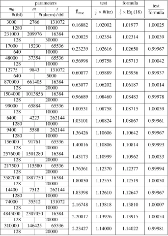
For each choice ofm0andt, we created multiple perfect DP tables fromm0starting
points. For each pre-computation table, we generated as many online chains as was required to observe a sufficiently large number of alarms. For each merge, the associ-ated pre-computation chain was generassoci-ated, up to the point of merge, and the length of this chain segment was recorded. That is, the online chain record method, previously explained in Section 2.1, was used to terminate the chain regeneration at the point of chain merge, rather than at the ending point DP.
Table 2: The number one-way function iterations required to resolve each alarm for various parameters. (N=248; ˆt=15t).
parameters test formula
test formula
m0 m t ¯
Dmsc 1t×#(itr) 1t×Eq.(18)
#(tbl) #(alarm) / tbl
3000 2766 131072
0.16882 1.02002 1.01977 1.00025
1280 10000
231000 209976 16384
0.20025 1.02354 1.02314 1.00039
128 30000
17000 15230 65536
0.23239 1.02616 1.02650 0.99967
640 10000
48000 37354 65536
0.56998 1.05758 1.05713 1.00042
128 10000
12775 9843 131072
0.60077 1.05889 1.05956 0.99937
640 5000
870000 661405 16384
0.63077 1.06202 1.06187 1.00014
128 20000
1504000 1013856 16384
0.96689 1.08460 1.08483 0.99978
128 20000
99000 65884 65536
1.00531 1.08758 1.08715 1.00039
128 10000
6400 4223 262144
1.03101 1.08824 1.08867 0.99961
1280 10000
9400 5588 262144
1.36426 1.10606 1.10642 0.99967
1280 10000
156000 91761 65536
1.40016 1.10806 1.10814 0.99993
128 20000
2576000 1501280 16384
1.43173 1.10999 1.10962 1.00033
128 20000
217500 115580 65536
1.76361 1.12370 1.12377 0.99994
128 20000
3587000 1887750 16384
1.80030 1.12553 1.12519 1.00030
128 20000
14400 7512 262144
1.83398 1.12610 1.12647 0.99967
1280 10000
74000 35512 131072
2.16748 1.13818 1.13810 1.00007
128 10000
4845000 2307050 16384
2.20017 1.13976 1.13915 1.00054
128 20000
310000 146425 65536
2.23427 1.14000 1.14022 0.99981


![Figure 5: The value tN| ¯DM| = ¯DmscD¯cr as predicted by [16] (solid) and the current work(dashed)](https://thumb-us.123doks.com/thumbv2/123dok_us/7885930.1308460/39.612.223.389.122.232/figure-value-dmscd-predicted-solid-current-work-dashed.webp)
