ABSTRACT
MCMAHON, MALLORY ELISE. Unsupervised Learning Models for Dual-Domain Data with Proximal Geographic Clustering. (Under the direction of Mansoor Haider.)
A dual-domain data set is comprised of two distinct sets of features, with one set consisting of
geographic or spatial data and the other consisting of attribute data. This type of data is ubiquitous
across a wide spectrum of disciplines, yet identifying meaningful clusters within dual-domain data
sets is often non-trivial. Conventional clustering methods often rely exclusively on similarity in the
geographic domain when interpreting clusters, even though the algorithm was likely trained on
the entire data set. While this approach may be effective for identifying well-delineated geographic
groupings, it does not account for instances where data observations that are similar in the attribute
domain are geographically dispersed. Some recent works have proposed multi-pass approaches
that determine similarity in each domain individually, then iteratively merge and tune the clusters
to resolve inter-domain discrepancies. In this work, we developed a tailored unsupervised learning
methodology based on the Self-Organizing Map (SOM) algorithm that is specifically designed to
address the challenges of dual-domain clustering in an automated way. Our framework incorporates
domain-specific biasing parameters into the SOM training that are subsequently optimized via an
objective function.
The tailored learning methodology in this work, referred to as the Tailored SOM, incorporated
the use of a 2-dimensional, 3×3 rectangular SOM structure that was trained on dual-domain data via
a reformulated Euclidean distance measure. This reformulation considers and measures similarity
using domain-specific biasing parameters, which allow for feature weighting and better evaluation
of inter-domain data relationships. To optimize the values of these parameters, we constructed an
objective function defined with quantities derived from the clustering projection in the geographic
domain as well as statistical measures of the attribute clusters. The choice of these quantities was
motivated directly by the overall goals of dual-domain clustering and designed to be sufficiently
versatile across applications. We prescribed an admissible space for the biasing parameters and
proposed two global methods for its traversal: a systematic grid search and the stochastic technique
To test the performance and robustness of the tailored learning methodology, we generated
several cases of synthetic dual-domain data with varying structure and complexity. To ensure
consistent and methodical algorithm assessment, we designed three metrics: theStable Score, the Inlier Score, and the notion ofGeographic Feasibility. We evaluated these metrics, along with the tailored objective function, to assess and compare the results obtained by the Tailored SOM and
two standard clustering algorithms, the Standard SOM and thek-Means algorithm. The evaluation of these metrics demonstrated that the results produced by the Tailored SOM were, by and large,
the most geographically desirable and feasible. Additionally, this analysis provided us with insight
into the relative tendencies, strengths, and limitations of the Tailored SOM, the Standard SOM and
thek-Means algorithm when applied to dual-domain data sets. Finally, we tested the capability of the Tailored SOM on a dual-domain data set consisting of geographically-ordered colorectal cancer
incidence rates in the state of California. With this data set, we further investigated the applicability
of a versatile objective function, the advantage of a tailored objective function, and the robustness
of the Tailored SOM and its associated learning methodology in the context of higher-dimensional
data. Our results demonstrated the unique capability of the Tailored SOM to identify both a
well-delineated geographic clustering and significant groupings of high and low cancer incidence. These
findings are significant in that they could provide the public health and epidemiology community
with a more holistic understanding of the relationships between geographic location, demographic
© Copyright 2020 by Mallory Elise McMahon
Unsupervised Learning Models for Dual-Domain Data with Proximal Geographic Clustering
by
Mallory Elise McMahon
A dissertation submitted to the Graduate Faculty of North Carolina State University
in partial fulfillment of the requirements for the Degree of
Doctor of Philosophy
Applied Mathematics
Raleigh, North Carolina
2020
DEDICATION
BIOGRAPHY
Mallory was born and raised in Southampton, New York. As an undergraduate, she studied
Mathe-matics at High Point University in High Point, North Carolina and Spanish at the Spanish American
Institute of International Education in Sevilla, Spain. In 2014, she graduatedsumma cum laudewith All-University Honors and had hopes of soon pursuing a Ph.D. In 2015, she moved to Raleigh, North
Carolina and began her graduate studies in Applied Mathematics at North Carolina State University.
Aside from math, Mallory loves traveling, cooking, quoting The Office, and spending sunny Saturday
ACKNOWLEDGEMENTS
I would like to sincerely thank my advisor, Dr. Mansoor Haider, for his guidance, support, and
friendship throughout my graduate studies. His mentorship, enthusiasm, and encouragement were
integral to the successful completion of this work. I would also like to thank the members of my
committee, Dr. Kevin Flores, Dr. Arvind Saibaba, and Dr. Ralph Smith for their feedback and support.
Additionally, I would like to acknowledge that this work was supported in part by a Statistical and
Applied Mathematical Sciences Institute (SAMSI) Graduate Fellowship, and the National Science
Foundation (NSF) Award DMS-1639521.
I would like to lovingly thank my family for their unwavering encouragement, support, and
dependability. For instilling in me the confidence to dream big, and the work ethic and drive to
transform my goals into reality. I could never have done this without you.
I am forever indebted to my truly incredible friends (and fellowModelers Anon), Michael Lavigne, Tricity Andrew, Jared Cook, and Sangeeta Warrier for being by my side every step of the way
these last five years. For sharing your brilliance, for finding laughter and fun among all the failures,
for teaching me everything I know about MATLAB, and for always, always believing in me.
Finally, I owe an enormous thank-you to my partner, Rob, for his unyielding love and patience,
and his unmatched ability to make me smile. For always taking an interest in my work, seeing me
TABLE OF CONTENTS
LIST OF TABLES . . . vii
LIST OF FIGURES. . . xii
Chapter 1 Introduction. . . 1
1.1 Motivation . . . 1
1.2 Definition of a Successful Clustering . . . 2
1.3 A Review of Literature on Dual-Domain Clustering Methods . . . 3
1.4 Tailored Clustering using Self-Organizing Maps . . . 5
Chapter 2 Unsupervised Learning Algorithms. . . 7
2.1 Unsupervised Learning . . . 7
2.2 Self-Organizing Map . . . 9
2.2.1 SOM Parameters . . . 12
2.3 k-Means . . . 13
2.3.1 Determining the Optimalk . . . 17
2.4 Tailored Unsupervised Learning . . . 23
Chapter 3 Tailored Clustering of Dual-Domain Data using Self-Organizing Maps . . . 25
3.1 A Tailored Self-Organizing Map . . . 25
3.2 Designing an Objective Function . . . 28
3.3 Optimizing the Objective Function . . . 33
Chapter 4 Evaluating the Tailored Self-Organizing Map with Synthetic Data . . . 39
4.1 Approach . . . 39
4.2 Generation of Dual-Domain Synthetic Data . . . 40
4.3 Synthetic Data: Case 1 . . . 45
4.3.1 Tailored versus Standard Clustering Results: Case 1 . . . 47
4.3.2 Algorithm Assessment: Case 1 . . . 55
4.4 Synthetic Data: Case 2 . . . 67
4.4.1 Tailored versus Standard Clustering Results: Case 2 . . . 69
4.4.2 Algorithm Assessment: Case 2 . . . 73
4.5 Synthetic Data: Case 3 . . . 81
4.5.1 Tailored versus Standard Clustering Results: Case 3 . . . 83
4.5.2 Algorithm Assessment: Case 3 . . . 88
4.5.3 Optimization via Simulated Annealing . . . 93
4.6 Discussion . . . 98
Chapter 6 Conclusions . . . .124
6.1 Conclusions and Summary of Contributions . . . 124
6.2 Future Work . . . 127
LIST OF TABLES
Table 3.1 Clustering-based quantities used in construction of objective function. . . 29
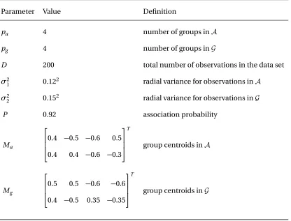
Table 4.1 Parameters used to generate synthetic dual-domain data. . . 44 Table 4.2 Parameter values used to manufacture the first case of synthetic data. . . 46 Table 4.3 Parameters and design choices prescribed for training the Tailored SOM on
Case 1 synthetic data. . . 48 Table 4.4 Stable Score and Inlier Score Algorithm . . . 57 Table 4.5 Values of the geographic objective functionJg (equation (3.1)) for the
cluster-ings determined by the Tailored SOM, the Standard SOM, and thek-Means algorithm (k =6) on the example Case 1 data set depicted in Figure 4.4. . . 58 Table 4.6 Stable Scores (SS) and Inlier Scores (IS) for the clustering of the example Case
1 data set depicted in Figure 4.4 obtained by the Tailored SOM (Figure 4.6 (c)), the Standard SOM (Figure 4.6 (d)), andk-Means fork =6 (Figure 4.9 (d)). Each of the “Cluster" columns contains the scores for the best-matching cluster to one of the 4 stable groups determined for this example data. The “Mean" column contains the mean Stable Score and mean Inlier Score across all four stable groups for each algorithm. The “Median" column contains the median Stable Score and median Inlier Score across all four stable groups for each algorithm. . . 59 Table 4.7 The percentage of Case 1 realizations for which a geographically feasible
clustering was achieved by the Tailored SOM, the Standard SOM, and the k-Means algorithm. . . 60 Table 4.8 The results of performing Dunn’s multiple comparison test (as a follow-up to
the Kruskal-Wallis test) to test for statistically significant differences among the distributions ofJg values obtained by the Tailored SOM, the Standard SOM, and thek algorithm. . . 61 Table 4.9 Mean Stable Score, Mean Inlier Score, and Geographic Feasibility results for
the Tailored SOM (TSOM), Standard SOM (SSOM), andk-Means Algorithm for 20 realizations of Case 1 synthetic data. Mean Stable Scores and Mean Inlier Scores were computed based on four stable groups determined with n =2.5 standard deviations (Step 1(b), Table 4.4). In the “Geographically Feasible?" columns, ’Y’ indicates the result is geographically feasible and ’N’ indicates the result is not geographically feasible. . . 64 Table 4.10 Parameter values used to manufacture the second case of synthetic data. . . . 68 Table 4.11 Parameters and design choices prescribed for training the Tailored SOM on
Case 2 synthetic data. . . 70 Table 4.12 Values of the geographic objective functionJg (equation (3.1)) for the
Table 4.13 Stable Scores (SS) and Inlier Scores (IS) for the clustering of the example Case 2 data set depicted in Figure 4.16 obtained by the Tailored SOM (Figure 4.17 (c)), the Standard SOM (Figure 4.17 (d)), andk-Means fork=7 (Figure 4.19 (d)). Each of the “Cluster" columns contains the scores for the best-matching cluster to one of the 4 stable groups determined for this example data. The “Mean" column contains the mean Stable Score and mean Inlier Score across all four stable groups for each algorithm. The “Median" column contains the median Stable Score and median Inlier Score across all four stable groups for each algorithm. The red text color is used to denote an algorithm that produced a geographically unfeasible clustering for this example Case 2 data set. . . 75 Table 4.14 The percentage of Case 2 realizations for which a geographically feasible
clustering was achieved by the Tailored SOM, the Standard SOM, and the k-Means algorithm. . . 75 Table 4.15 The results of performing Tukey’s multiple comparison test (as a follow-up to
the one-way ANOVA test) to test for statistically significant differences among the distributions ofJg values obtained by the Tailored SOM, the Standard SOM, and thek algorithm for the Case 2 data. . . 76 Table 4.16 Parameter values used to manufacture the third case of synthetic data. . . 82 Table 4.17 Values of the geographic objective functionJg (equation (3.1)) for the
cluster-ings determined by the Tailored SOM, the Standard SOM, and thek-Means algorithm (k =4) on the example Case 3 data set depicted in Figure 4.24. . . . 88 Table 4.18 Stable Scores (SS) and Inlier Scores (IS) for the clustering of the example Case
3 data set depicted in Figure 4.24 obtained by the Tailored SOM (Figure 4.25 (c)), the Standard SOM (Figure 4.25 (d)), andk-Means fork=4 (Figure 4.27 (d)). Each of the “Cluster" columns contains the scores for the best-matching cluster to one of the 5 stable groups determined for this example data. The “Mean" column contains the mean Stable Score and mean Inlier Score across all five stable groups for each algorithm. The “Median" column contains the median Stable Score and median Inlier Score across all five stable groups for each algorithm. The red text color is used to denote the algorithms that produced a geographically unfeasible clustering for this example Case 3 data set. . . 88 Table 4.19 The percentage of Case 3 realizations for which a geographically feasible
clustering was achieved by the Tailored SOM, the Standard SOM, and the k-Means algorithm. . . 89 Table 4.20 The results of performing Dunn’s multiple comparison test (as a follow-up to
the Kruskal-Wallis test) to test for statistically significant differences among the distributions ofJg values obtained by the Tailored SOM, the Standard SOM, and thek-Means algorithm for Case 3 data. . . 90 Table 4.21 Values of the geographic objective functionJg (equation (3.1)) for the
clus-terings determined by: the Tailored SOM with optimalq∗
Table 5.1 Colorectal cancer incidence and demographic features selected for clustering and/or analysis obtained from the 2001-2016 SEER database. . . 103 Table 5.2 Parameters and design choices prescribed for training the Tailored SOM on
theR4subset of the colorectal cancer data consisting of latitude, longitude, MW Rate, and MB Rate features. . . 107 Table 5.3 A depiction of the results of performing pairwise statistical testing (either the
ANOVA test followed by the Tukey multiple comparison test, or the Kruskal-Wallis test followed by Dunn’s test) on the top 4 largest clusters identified by the Tailored SOM (Figure 5.3 (a)). The top 4 largest clusters are denoted as “C1T",“C2T",“C3T",“C4T" and correspond to the clusters referenced in the legend of Figure 5.3 (a). To aid in the visualization of these results, we have highlighted in yellow each pairwise comparison that is statistically significant at theα=0.05 significance level. . . 110 Table 5.4 A depiction of the results of performing pairwise statistical testing (either the
ANOVA test followed by the Tukey multiple comparison test, or the Kruskal-Wallis test followed by Dunn’s test) on the top 4 largest clusters identified by the Standard SOM (Figure 5.3 (b)). The top 4 largest clusters are denoted as “C1S",“C2S",“C3S",“CS
4" and correspond to the clusters referenced in the legend of Figure 5.3 (b). To aid in the visualization of these results, we have highlighted in yellow each pairwise comparison that is statistically significant at theα=0.05 significance level. . . 111 Table 5.5 A depiction of the results of performing pairwise statistical testing (either the
ANOVA test followed by the Tukey multiple comparison test, or the Kruskal-Wallis test followed by Dunn’s test) on the top 4 largest clusters identified by thek-Means algorithm fork=9 (Figure 5.3 (d)). The top 4 largest clusters are denoted as “C1k9",“C2k9",“C3k9",“Ck9
4 " and correspond to the clusters refer-enced in the legend of Figure 5.3 (d). To aid in the visualization of these results, we have highlighted in yellow each pairwise comparison that is statistically significant at theα=0.05 significance level. . . 111 Table 5.6 Values of the geographic objective functionJg (as defined in Section 5.2.1)
and the percentage of pairwise cluster comparisons (of the 4 largest clusters, across the 8 attribute features) that are significantly different (σA) for the clusterings determined by the Tailored SOM, the Standard SOM, and the k-Means algorithm (k =9) on theR4subset of the cancer incidence data. . . . 111 Table 5.7 The fraction (reported as a percentage) of the total California area occupied
by overlapping cluster regions PAi,j ˜
A , fori,j =1, ..,C andi 6= j
Table 5.8 A depiction of the results of performing pairwise statistical testing (either the ANOVA test followed by the Tukey multiple comparison test, or the Kruskal-Wallis test followed by Dunn’s test) on the top 4 largest clusters identified by the Tailored SOM via the combination objective function Jc (Figure 5.5 (a)). The top 4 largest clusters are denoted as “C1T,c",“C2T,c",“C3T,c",“C4T,c" and correspond to the clusters referenced in the legend of Figure 5.5 (a). To aid in the visualization of these results, we have highlighted in yellow each pairwise comparison that is statistically significant at theα=0.05 significance level. . . 117 Table 5.9 A depiction of the results of performing pairwise statistical testing (either the
ANOVA test followed by the Tukey multiple comparison test, or the Kruskal-Wallis test followed by Dunn’s test) on the top 4 largest clusters identified by the Tailored SOM via the geographic objective function Jg (Figure 5.5 (b)). The top 4 largest clusters are denoted as “C1T,g",“C2T,g",“C3T,g",“C4T,g" and correspond to the clusters referenced in the legend of Figure 5.5 (b). To aid in the visualization of these results, we have highlighted in yellow each pairwise comparison that is statistically significant at theα=0.05 significance level. . . 118 Table 5.10 The fraction (reported as a percentage) of the total California area occupied
by overlapping cluster regions PAAi˜,j, fori,j =1, ..,C andi 6= jand the percentage of pairwise cluster comparisons (of the 4 largest clusters, across the 8 attribute features) that are significantly different (σA) for the cluster-ings determined by the Tailored SOM, the Standard SOM, and thek-Means algorithm (fork=6, 9) on theR6subset of the cancer incidence data. . . 121 Table 5.11 A depiction of the results of performing pairwise statistical testing (either the
ANOVA test followed by the Tukey multiple comparison test, or the Kruskal-Wallis test followed by Dunn’s test) on the top 4 largest clusters identified by the Tailored SOM via the combination objective functionJc for theR6data subset (Figure 5.6 (a)). The top 4 largest clusters are denoted as “CT
1",“C2T",“C3T",“C4T" and correspond to the clusters referenced in the legend of Figure 5.6 (a). To aid in the visualization of these results, we have highlighted in yellow each pairwise comparison that is statistically significant at theα=0.05 significance level. . . 121 Table 5.12 A depiction of the results of performing pairwise statistical testing (either the
ANOVA test followed by the Tukey multiple comparison test, or the Kruskal-Wallis test followed by Dunn’s test) on the top 4 largest clusters identified by the Standard SOM for theR6data subset (Figure 5.6 (b)). The top 4 largest clusters are denoted as “C1S",“C2S",“C3S",“CS
4" and correspond to the clus-ters referenced in the legend of Figure 5.6 (b). To aid in the visualization of these results, we have highlighted in yellow each pairwise comparison that is statistically significant at theα=0.05 significance level. . . 121 Table 5.13 A depiction of the results of performing pairwise statistical testing (either the
Table 5.14 A depiction of the results of performing pairwise statistical testing (either the ANOVA test followed by the Tukey multiple comparison test, or the Kruskal-Wallis test followed by Dunn’s test) on the top 4 largest clusters identified by thek-Means algorithm withk=9 for theR6data subset (Figure 5.6 (c)). The top 4 largest clusters are denoted as “C1k9",“C2k9",“C3k9",“Ck9
LIST OF FIGURES
Figure 1.1 An example of a dual-domain data set, projected into the geographic domain
G, featuring a geographic constraint in the form of a river. In this example, there are geographic data observations located on each side of the river that correspond to one of three attribute groups (groupings in the attribute domainA). We use the marker type/color (red circle, green x, black diamond) to indicate each geographic data observation’s association with an attribute group. . . 2 Figure 1.2 A depiction of possible geographic clusterings obtained via standard
clus-tering algorithms that: (a) only consider the data in the geographic domain (G) during training, and (b) consider and weight all features in the data set equally (in both domainsG,A) during training. . . 4
Figure 2.1 A depiction of a data set suited for: (a) an elementary supervised classifica-tion problem, and (b) an unsupervised clustering algorithm. The marker types/colors in (a) denote theknownlabels of each data observation, which are used to train a classifier. In contrast, observations in (b) have the same marker type/color, thus demonstrating the lack of available data labels in an unsupervised clustering problem. . . 8 Figure 2.2 Illustration of a 3 x 3 rectangular lattice SOM with select weight vectors. . . . 10 Figure 2.3 Illustration of a 3 x 3 triangular lattice SOM with select weight vectors. . . 12 Figure 2.4 Illustration of implementing the first few steps of thek-Means algorithm on
a two-dimensional data set. . . 16 Figure 2.5 Two-dimensional data set generated from 4 cluster distributions with radial
varianceσ=0.22. . . 19 Figure 2.6 Elbow Method results for data depicted in Figure 2.5: total WSS as a function
ofk. . . 19 Figure 2.7 Average Silhouette Method results for data depicted in Figure 2.5: averageSi
as a function ofk. . . 20 Figure 2.8 Two-dimensional data set generated from 4 cluster distributions with radial
varianceσ=0.252. . . 21 Figure 2.9 Elbow Method results for data depicted in Figure 2.8: total WSS as a function
ofk. . . 22 Figure 2.10 Average Silhouette Method results for data depicted in Figure 2.8: averageSi
as a function ofk. . . 22
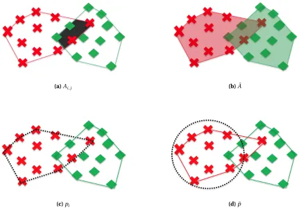
Figure 3.1 An example of a dual-domain data set, clustered by the Tailored SOM and projected intoG. Once clustered and projected, we construct the convex hull of each geographic cluster. The convex hulls act as boundaries for the clusters and create a geographic region for each cluster. . . 30 Figure 3.2 An illustration of various terms (defined in Table 3.1) to be included in the
Figure 3.3 A depiction of the optimization framework for determining the optimal parameter setq∗= [α∗,β∗]for a given data set via the Tailored SOM (TSOM)
algorithm and an objective functionJg α,β
. . . 35
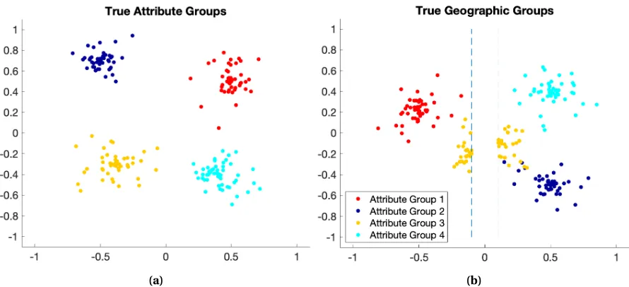
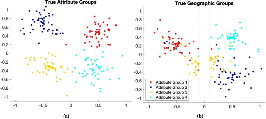
Figure 4.1 A sample dual-domain data arrangement generated from the parameter values specified byQ1,Ma,1, andMg,1projected into the two-dimensional attribute domain (shown in (a)) and the two-dimensional geographic do-main (shown in (b)). The marker colors in each subfigure are used to indicate the inter-domain correspondence/association between the geographic ob-servations and the attribute obob-servations. . . 42 Figure 4.2 A second sample dual-domain data arrangement generated from the
param-eter values specified byQ2,Ma,1, andMg,1projected into the two-dimensional attribute domain (shown in (a)) and the two-dimensional geographic do-main (shown in (b)). The marker colors in each subfigure are used to indicate the inter-domain correspondence/association between the geographic ob-servations and the attribute obob-servations. . . 43 Figure 4.3 A third sample dual-domain data arrangement generated from the
parame-ter values specified byQ3,Ma,1, andMg,1projected into the two-dimensional attribute domain (shown in (a)) and the two-dimensional geographic do-main (shown in (b)). The marker colors in each subfigure are used to indicate the inter-domain correspondence/association between the geographic ob-servations and the attribute obob-servations. . . 44 Figure 4.4 A sample Case 1 data set generated from the parameter values defined in
Ta-ble 4.2 projected into the two-dimensional attribute domain (Subfigure (a)) and the two-dimensional geographic domain (Subfigure (b)). The marker colors in each subfigure are used to indicate the inter-domain correspon-dence between the geographic observations and the attribute observations. 47 Figure 4.5 An illustration of the function values attained byJg α,β
(equation (3.1)) at eachα,βpair (equation (4.1)) evaluated during the global grid search for the Case 1 data set depicted in Figure 4.4. Each function value is denoted by the color of the square. . . 49 Figure 4.6 The geographic clusterings for the example Case 1 data set (shown in (a)
Figure 4.8 An illustration of the geographic clustering of the example Case 1 data set (shown in (a) and (b)) obtained with thek-Means algorithm for (c)k=4, (d) k=5, (e)k =6, and (f )k =7, as recommended by the Elbow and Average Silhouette Methods. . . 53 Figure 4.9 The geographic clusterings for the example Case 1 data set (shown in 4.4)
obtained from: (c) training the Tailored SOM algorithm withq∗= [0.8, 1.1] and (d) training thek-Means algorithm withk = 6. Post clustering, we apply the convex hull boundaries to each geographic cluster containing at least 2 data observations. For this data set, the Tailored SOM (shown in (c)) identified 7 geographic clusters, denoted by marker color, and thek-Means algorithm (shown in (d)) identified 6 geographic clusters, also denoted by marker color. . . 54 Figure 4.10 A depiction of the first iteration of the stable group construction for a known
geographic group. In the example Case 1 data set shown in (a), we consider all observations associated with Attribute Group 4 (cyan). In (b) we depict the centroid of the cyan observations with a black ‘x’ and 2.5-standard de-viations (radially) from the centroid with a black dashed circle. We identify 4 observations that fall outside this circle (each noted with a black arrow. Each of these outlying observations would be removed from the cyan stable group at this iteration of the construction process. This process repeats by updating the centroid and the 2.5-standard deviation boundary, and remov-ing outliers until the population of the stable group no longer changes. Once complete, the stable group is considered the set of core observations for that particular geographic group and can be used in computing the Stable and Inlier Scores (defined in Table 4.4). . . 56 Figure 4.11 An example of a geographically unfeasible clustering produced by thek
-Means algorithm (withk=5) on a Case 1 synthetic data set. We make this determination based on how the convex boundaries of several geographic clusters span across the vertical constraint. . . 60 Figure 4.12 The box plots of theJgvalues obtained by each algorithm: the Tailored SOM
(TSOM), the Standard SOM (SSOM), andk-Means for all realizations of Case 1 data. . . 61 Figure 4.13 A depiction of the values ofJg obtained for each realization of the Case 1
Figure 4.14 For each realization of Case 1 data, we compute the difference in mean Stable Score (shown in (a)) and mean Inlier Score (shown in (b)) achieved by the optimized Tailored SOM (TSOM) versus the Standard SOM (SSOM). A positive score difference indicates a realization for which the TSOM achieved a higher score than the SSOM. Additionally, we plot the mean score differ-ence across all realizations (solid red line) and±1 standard deviation of the mean score differences (dashed red lines). The solid blue line indicates no difference in the mean scores. . . 65 Figure 4.15 For each realization of Case 1 data, we compute the difference in mean Stable
Score (shown in (a)) and mean Inlier Score (shown in (b)) achieved by the optimized Tailored SOM (TSOM) versus thek-Means algorithm. A positive score difference indicates a realization for which the TSOM achieved a higher score than thek-Means algorithm. Additionally, we plot the mean score difference across all realizations (solid red line) and±1 standard deviation of the mean score differences (dashed red lines). The solid blue line indicates no difference in the mean scores. . . 66 Figure 4.16 A sample Case 2 data set generated from the parameter values defined in
Ta-ble 4.10 projected into the two-dimensional attribute domain (shown in (a)) and the two-dimensional geographic domain (shown in (b)). The marker col-ors in each subfigure are used to indicate the inter-domain correspondence between the geographic observations and the attribute observations. . . 69 Figure 4.17 The geographic clusterings obtained for the example Case 2 data set (shown
in (a), (b)) from training the Tailored SOM algorithm withq∗= [0.75, 1.1] (shown in (c)) and the Standard SOM algorithm (shown in (d)). Post clus-tering, we apply the convex hull boundaries to each geographic cluster containing at least 2 data observations. For this data set, the Tailored SOM (shown in (c)) identified 9 geographic clusters, denoted by marker color, and the Standard SOM (shown in (d)) identified 9 geographic clusters, also denoted by marker color. . . 71 Figure 4.18 Average Silhouette Method results for the Case 2 data set depicted in Figure
4.16. This method relies on the silhouette coefficient (Si) (equation (2.4)) of each observation. The Average Silhouette Method suggests choosing the value ofkthat maximizes the average silhouette coefficient. In this example, the optimal value isk=7. . . 72 Figure 4.19 The geographic clusterings obtained for the example Case 2 data set (shown
in (a,b)) from training the Tailored SOM algorithm withq∗ = [0.75, 1.1]
Figure 4.21 A depiction of the values ofJg obtained for each realization of the Case 2 data by (a): the Tailored SOM versus the Standard SOM and (b): the Tai-lored SOM versus thek-Means algorithm. For each comparison, we sort the function values in ascending order and use the marker colors to indi-cate the geographic feasibility of each realization. A blue marker indiindi-cates a geographically feasible result and a red marker indicates a geographically unfeasible result. In each plot, the solid plotted line corresponds to the re-sults obtained from the Tailored SOM and the dashed line corresponds to the results obtained by the Standard SOM (a) or thek-Means algorithm (b). 77 Figure 4.22 For each realization of Case 2 data, we compute the difference in mean
Stable Score (Subfigure (a)) and mean Inlier Score (Subfigure (b)) achieved by the optimized Tailored SOM (TSOM) versus the Standard SOM (SSOM). A positive score difference indicates a realization for which the TSOM achieved a higher score than the SSOM. Additionally, we plot the mean score differ-ence across all realizations (solid red line) and±1 standard deviation of the mean score differences (dashed red lines). The solid blue line indicates no difference in the mean scores. . . 79 Figure 4.23 For each realization of Case 2 data, we compute the difference in mean Stable
Score (Subfigure (a)) and mean Inlier Score (Subfigure (b)) achieved by the optimized Tailored SOM (TSOM) versus thek-Means algorithm. A positive score difference indicates a realization for which the TSOM achieved a higher score than thek-Means algorithm. Additionally, we plot the mean score difference across all realizations (solid red line) and±1 standard deviation of the mean score differences (dashed red lines). The solid blue line indicates no difference in the mean scores. . . 80 Figure 4.24 A sample Case 3 data set generated from the parameter values defined in
Table 4.2 projected into the two-dimensional attribute domain (shown in (a)) and the two-dimensional geographic domain (shown in (b)). The marker colors in each subfigure are used to indicate the inter-domain correspon-dence between the geographic observations and the attribute observations. For this case, there are two distinct geographic groups (shown in (b)) that correspond to the same attribute group (yellow group in (a)). . . 81 Figure 4.25 The geographic clusterings obtained for the example Case 3 data set (shown
in (a), (b)) from training the Tailored SOM algorithm withq∗= [0.75, 1.20] (shown in (c)) and the Standard SOM algorithm (shown in (d)). Post clus-tering, we apply the convex hull boundaries to each geographic cluster containing at least 2 data observations. For this data set, the Tailored SOM (shown in (c)) identified 8 geographic clusters, denoted by marker color, and the Standard SOM (shown in (d)) identified 9 geographic clusters, also denoted by marker color. . . 84 Figure 4.26 Results of the Elbow Method (shown in (a)) and the Average Silhouette
Figure 4.27 The geographic clusterings obtained for the example Case 3 data set (shown in (a,b)) from training the Tailored SOM algorithm withq∗ = [0.75, 1.20]
(shown in (c)) and thek-Means algorithm withk=4 (shown in (d)). Post clustering, we apply the convex hull boundaries to each geographic cluster containing at least 2 data observations. . . 86 Figure 4.28 An illustration of the geographic clustering of the example Case 3 data set
(shown in (a,b)) obtained with thek-Means algorithm fork =5 (shown in (c)) andk=6 (shown in (d)). . . 87 Figure 4.29 The box plots of theJgvalues obtained by each algorithm: the Tailored SOM
(TSOM), the Standard SOM (SSOM), andk-Means for all realizations of Case 3 data. . . 90 Figure 4.30 A depiction of the values ofJg obtained for each realization of the Case 3
data by (a): the Tailored SOM versus the Standard SOM and (b): the Tai-lored SOM versus thek-Means algorithm. For each comparison, we sort the function values in ascending order and use the marker colors to indi-cate the geographic feasibility of each realization. A blue marker indiindi-cates a geographically feasible result and a red marker indicates a geographically unfeasible result. In each plot, the solid plotted line corresponds to the re-sults obtained from the Tailored SOM and the dashed line corresponds to the results obtained by the Standard SOM (a) or thek-Means algorithm (b). 91 Figure 4.31 For each realization of Case 3 data, we compute the difference in mean
Stable Score (Subfigure (a)) and mean Inlier Score (Subfigure (b)) achieved by the optimized Tailored SOM (TSOM) versus the Standard SOM (SSOM). A positive score difference indicates a realization for which the TSOM achieved a higher score than the SSOM. Additionally, we plot the mean score differ-ence across all realizations (solid red line) and±1 standard deviation of the mean score differences (dashed red lines). The solid blue line indicates no difference in the mean scores. . . 92 Figure 4.32 For each realization of Case 3 data, we compute the difference in mean Stable
Score (Subfigure (a)) and mean Inlier Score (Subfigure (b)) achieved by the optimized Tailored SOM (TSOM) versus thek-Means algorithm. A positive score difference indicates a realization for which the TSOM achieved a higher score than thek-Means algorithm. Additionally, we plot the mean score difference across all realizations (solid red line) and±1 standard deviation of the mean score differences (dashed red lines). The solid blue line indicates no difference in the mean scores. . . 93 Figure 4.33 The geographic clusterings obtained for the example Case 3 data set (shown
in (a), (b)) from training the Tailored SOM algorithm with the optimal param-eter set identified by the global grid search,q∗
Figure 4.34 To compare the clusterings of the Case 3 data realizations achieved by the Tailored SOM via a global grid search (GS) and the Tailored SOM via the Simulated Annealing algorithm (SA), we depict the box plots of theJg values obtained by each optimization approach (shown in (a)). Additionally, we de-pict of the values ofJg obtained for each realization by the two optimization approaches (shown in (b)). For this comparison, we sort the function values in ascending order and use the marker colors to indicate the geographic feasibility of each realization. A blue marker indicates a geographically fea-sible result and a red marker indicates a geographically unfeafea-sible result. The solid plotted line corresponds to the results obtained from the Tailored SOM via the global grid search and the dashed line corresponds to the re-sults obtained by the Tailored SOM via the Simulated Annealing algorithm. Lastly, we depict the difference in mean Stable Scores and mean Inlier Scores achieved by the Tailored SOM optimized with the global grid search versus the Tailored SOM optimized via the Simulated Annealing Algorithm (shown in (c,d)). . . 97
Figure 5.1 A scatter plot of the representative longitude, latitude pair for each county, labeled with the county name. To maintain consistency with standard map views, we have longitude on the horizontal axis and latitude on the vertical axis. . . 104 Figure 5.2 A depiction of the box plots of the data from various features in the attribute
domain. In (a), we depict the box plots for the colorectal cancer incidence rates by group: Male/White Rate (MW Rate), Male/Black Rate (MB Rate), Female/White Rate (FW Rate), Female/Black Rate (FB Rate). In (b), we depict the box plots for the features related to demographic information: Percent Male (Perc M), Median Male Age (Age M), Median Female Age (Age F). In (c), we depict the box plot for the Population Density. . . 105 Figure 5.3 The geographic clusterings obtained for 4-dimensional case of the colorectal
cancer data with features: latitude, longitude, MW Rate, and MB Rate. These results are from training the Tailored SOM algorithm withq∗= [0.75, 1.25]
ob-tained via the geographic objective functionJg (shown in (a)), the Standard SOM algorithm (shown in (b)), thek-Means algorithm withk=5 (shown in (c)), and thek-Means algorithm withk=9. Post clustering, we apply the convex hull boundaries to each geographic cluster containing at least 2 data observations. . . 109 Figure 5.4 A depiction of some of the results obtained by the Tailored SOM
cluster-ing (shown in Figure 5.3 (a)). Each plot shows the data pertaincluster-ing to select features (Population Density, MW Rate, MB Rate, and FW Rate) that was assigned to first largest cluster (Cluster 1), the second largest cluster (Cluster 2), and all data pertaining to that feature. . . 113 Figure 5.5 The geographic clusterings obtained for 4-dimensional case of the
colorec-tal cancer data (with features: latitude, longitude, MW Rate, MB Rate) from training the Tailored SOM algorithm withq∗= [0.75, 1.1]obtained via the
CHAPTER
1
INTRODUCTION
1.1
Motivation
In this thesis we consider data from a dual-domain configuration. The configuration consists of an
attribute domainAand a geographic domainG. The attribute domain may contain information
re-lated to quantitative or measurable qualitative features. The geographic domainGprovides location
information for each observation inA. We allow the definition of geographic to be flexible, thusG
could provide data pertaining to physical locations, or "digital" locations, i.e., relative closeness on
a social network map or similarity in web-based activity, as described in[12]. Each dual-domain
data observationd~is a concatenation of all features from both domains, i.e.,d~= [a~,g~]wherea~∈A,
~
g∈G. An example of this dual-domain configuration, projected into the geographic domainGis illustrated in Figure 1.1. In this example, each point is an observation fromG, in the form of an(x,y) location pair, with the marker type indicating its true group in the attribute domainG. This example
Figure 1.1An example of a dual-domain data set, projected into the geographic domainG, featuring a geographic constraint in the form of a river. In this example, there are geographic data observations located on each side of the river that correspond to one of three attribute groups (groupings in the attribute domain
A). We use the marker type/color (red circle, green x, black diamond) to indicate each geographic data observation’s association with an attribute group.
We aim to find a clustering of a data set with observations of the formd~= [a~,g~]that is both telling of the intrinsic structure of the attribute domainAand is geographically useful. In other
words, the goal is to identify clusters of “like-minded" individuals (data observations) that are
geographically proximal. We loosely define a geographically useful cluster as one whose boundaries
do not span across geographic barriers or constraints and whose coverage area has minimal overlap
with other clusters. We view this problem as an unsupervised learning task, where neither the
observations from the attribute domainAnor the geographic domainGare labeled, therefore we
cannot train against a ground truth. Previous approaches to similar dual-domain (joint-domain)
clustering problems have been more heuristic in nature, requiring multiple phases and explicit
reliance on geographic constraints[24, 25, 27]. We, instead, view this as an optimization problem by
introducing an objective function directly motivated by the modeling application.
set grows. By definition, the observations of a data set undergoing a clustering regime are not labeled
nor classified a priori, i.e., there is neither an underlying ground truth nor “right answer" to train
the algorithm against[13]. With this type of task, we as researchers are responsible for designing a
notion of correctness based on either domain-specific knowledge, measurable qualities of the data
set itself, or desired cluster outcomes[1, 4, 44]. In the context of the dual-domain problem, we aim
to uncover a clustering that is both telling of the intrinsic structure of the attribute domainAand
is feasible in the geographic domainG. It is with this overarching goal in mind that we develop a
definition for correctness and construct the desired properties of the ideal clustering.
The reliance on synthetic data sets when building and testing our dual-domain clustering
approaches is especially advantageous when it comes to defining the desired properties of a right
answer. With synthetic data comes knowledge of underlying generating distributions, various levels
of noise within the data, and intended cluster arrangements inAandG. Based on this knowledge,
we can test the performance of an algorithm with scoring methods that consider quantities such as:
• the number of known primary groups identified,
• the number of outlying/anomalous observations assigned to each geographic cluster, and
• the degree to which geographic constraints present inG(such as the river depicted in Figure
4.3 (b)) were adhered to, i.e., not violated when geographic cluster boundaries are imposed.
In contrast to working with real data, we can reliably use these type of metrics when assessing
the clustering of synthetic data due to the level of control we have over its design. This control is
rooted in how we choose to prescribe values for the many parameters that are used in the synthetic
data set design process and allows for the creation of an assessment framework. Within this
frame-work, we can investigate how varying levels of noise and cluster separation affect the accuracy and
performance of our methods.
1.3
A Review of Literature on Dual-Domain Clustering Methods
Traditional clustering methods may approach a dual-domain problem by either: 1) only clustering
attribute domain and focusing exclusively on geographic proximity, or 2) using a standard algorithm
to cluster over the entire data set, weighting the features fromAandGequally when determining
similarity. Figure 1.2 (a,b) demonstrates possible outcomes of implementing methods 1) and 2),
re-spectively, on the sample dual-domain data set depicted in Figure 1.1. While the outcome presented
in Figure 1.2 (a) is mindful of geographic proximity, it is blind to attribute differences coexisting
within its clusters. The outcome presented in Figure 1.2 (b) is clearly problematic as it does not
account for the geographic constraint in the data set and instead favors attribute similarity, thus
producing a geographically unfeasible clustering.
(a) (b)
Figure 1.2A depiction of possible geographic clusterings obtained via standard clustering algorithms that: (a) only consider the data in the geographic domain (G) during training, and (b) consider and weight all
features in the data set equally (in both domainsG,A) during training.
Recent works[24, 25, 27]have proposed iterative, multi-pass methodologies to efficiently
cluster dual-domain data (also referred to as joint clustering). Such methods often require that the
clustering algorithms have explicit knowledge of constraints present in the geographic domain prior
to training, in order to produce a result that is geographically feasible (i.e., it does not violate said
constraints). In[25], Lin et al. proposes the Interlaced Clustering-Classification (ICC) algorithm to
(attribute) domain that correspond to compact geographic regions. Another multi-step approach
for clustering dual-domain data is proposed by Liao and Peng in[24]. Their method, called the
Clustering with Local Search (CLS) algorithm, proposes the construction of a connected graph,
based on given geographic constraints and requirements, which is subsequently used to determine
the placement of initial cluster representatives. From there, distances to nearby, connected data
observations are computed and “coarse" clusters are formed and then iteratively merged and tuned
[24]. In[27], Lo and Peng build upon the clustering methodology presented in[24]with their proposal
of thek-Means with Local Search (KLS) algorithm. The KLS algorithm consists of three phases which aim to (1) build a connected graph for representing constraints in the geographic domain, (2) apply
a coarse clustering to the data via an initial placement ofk or more cluster centroids, and (3) tune and merge the clusters, according to a cost function, until exactlyk clusters are identified.
A few commonalities among the existing dual-domain clustering methods outlined above
are:
• the use of multiple clustering and classification phases which focus exclusively on analyzing
the data in one of the two domains,
• the requirement of explicit knowledge of geographic constraints or definition for
geographi-cally connected, and
• the specification of the number of desired clusters.
1.4
Tailored Clustering using Self-Organizing Maps
In this thesis, we propose a tailored unsupervised learning methodology to efficiently cluster
dual-domain data sets that does not require explicit incorporation of the geographic constraints or a priori
specification of the number of desired clusters. Our algorithm aims to simultaneously cluster data in
both the geographic and attribute domain through the use of domain-specific biasing parameters,
the optimization of a tailored objective function, and the evaluation of generic geometric and
statistical quantities. In Chapter 2, we present an overview of unsupervised machine learning and a
thek-Means algorithm[30]. In Chapter 3, we propose and develop a novel tailored unsupervised learning algorithm called the Tailored SOM, which relies fundamentally on the Self-Organizing Map,
incorporates a reformulated distance measure, and employs a tailored objective function. Alongside
the development of this algorithm, we motivate the need for the tailored objective function, detail
the process through which we design its terms, and outline two methods for optimizing this function
within the clustering framework.
After fully developing the Tailored SOM, we build and consider three cases of synthetic
dual-domain data with varying structural characteristics and levels of noise that were specifically designed
to be useful dual-domain test cases. With each test case of synthetic data, we implement the
tai-lored unsupervised learning methodology presented in Chapter 3 and evaluate and compare its
performance against results obtained by the standard clustering algorithms presented in Chapter 2.
Furthermore, we propose and develop four novel metrics for evaluating and comparing algorithm
performance. We create two metrics that are based on properties of the synthetic-data set itself, a
third metric that accounts for geographic feasibility, and a fourth metric that quantifies geographic
desirability of a clustering. These metrics give structure and formality to our algorithm assessment
framework. These metrics, as novel contributions, are critical in the context of unsupervised
learn-ing, where there is neither a notion of "ground truth" nor a widely-accepted method for assessing
the validity of an algorithm’s output.
Finally, in Chapter 5, we consider a real dual-domain data set consisting of latitude/longitude
measurements, colorectal cancer incidence rates, and demographic information for counties in
the state of California. This data was obtained from the United State Census Bureau[43]and the
CDC’s National Program of Cancer Registries (NPCR) and the National Cancer Institute’s (NCI’s)
Surveillance, Epidemiology, and End Results (SEER) Program[37]. We use the cancer incidence data
CHAPTER
2
UNSUPERVISED LEARNING
ALGORITHMS
2.1
Unsupervised Learning
Unsupervised learning refers to the class of machine learning techniques used for analyzing
unla-beled data, i.e., a data set for which a known class or response for each observation is not provided.
Unsupervised learning algorithms aim to identify patterns, groups, and similarities within a data set
to ultimately cluster observations that have something in common[1, 32]. In the absence of explicit
information regarding whether an input observation belongs to one class or another, unsupervised
learning algorithms such as the Self-Organizing Map[18]andk-Means[30]rely on metrics such as distances between observations and the means of groups of observations to identify similarity and
groupings in an automated fashion. In contrast, supervised learning techniques, such as regression,
neural networks, and random forests, aim to learn the input-output relationship of labeled data
typically rely on an optimization regime to minimize an error function that uses the classes (outputs)
and the data observations (inputs) to learn the relationship between the two. Once the algorithm
has been trained and the input-output relationship has been learned, the supervised learning model
can be used to predict the output of future observations or classify unlabeled observations[1].
Figure 2.1 depicts a fundamental difference between supervised and unsupervised learning.
In an elementary supervised learning problem, as seen in Figure 2.1 (a), we have a standard two-class
classification task. The two different classes of data are depicted by the red circles and green x’s.
For this example, a supervised learning algorithm, such as the traditional Support Vector Machine
[7], would rely on the knowledge of the two labeled classes to learn, for instance, a linear separator
between them. Then, when new data is presented, the algorithm would use the learned separator to
classify the observations as belonging to one class or the other. This type of classification problem
can also be extended to multi-class (more than 2 classes) data sets. In an elementary unsupervised
learning task, as seen in Figure 2.1 (b), we are unaware of classes/labels, thus all data points are
depicted as purple circles with no distinction among them. For this example, an algorithm, such as
k-Means, would search for closeness among the data and decide on a clustering based on proximity. Depending on the application, new data can either be compared to the existing clusters and assigned
2.2
Self-Organizing Map
The standard Self-Organizing Map (SOM) is a type of Artificial Neural Network developed by Teuvo
Kohonen in the 1980s and was originally motivated by the human brain’s spatial organization and
how sensory signals are mapped into the cerebral cortex[17, 18]. The SOM functions similarly to a
sensory map, which details how various parts of the brain respond to spatially organized sensory
stimulation. The SOM learns an ordered, topology-preserving mapping from the input data to a
low-dimensional (typically 1- or 2-dimensional) map structure via a similarity-based competition.
This competitive learning algorithm uses a fully connected, low-dimensional map of nodes, depicted
in Figure 2.2, to cluster and produce a representation of the higher-dimensional input data. Each
node in the map is associated with a weight vector of dimension equal to that of the input data, and
with a set of neighboring nodes.
During the SOM training, weight vectors compete against each other to be chosen as the
“winner” based on the distance between each weight vector and the given data observation. Each
winning weight vector, and the weight vectors of its node’s neighbors, are then moved according to
their proximity to data observations deemed closest. The goal of this iterative, competitive process
is for each weight vector to become a “representative” for a cluster in the data. Additionally, the
data ultimately clustered to nodes that are neighbors on the SOM will be more similar than data
clustered to non-neighboring nodes. This property of neighboring nodes is unique to the SOM and
results in a representation of clusters that preserves the spatial organization of the original input
data space on the lower dimensional Self-Organizing Map.
Figure 2.2 depicts a two-dimensional, 3 x 3 rectangular lattice SOM consisting of nine nodes,
three sample input data observations, and select weight vectors. The edges of the SOM are used to
illustrate the neighborhood connections between nodes. Thus, any two nodes that are connected
with an edge are considered neighbors and will be treated accordingly during the competitive
learning. The weight vectors, a few of which are shown as dashed lines in Figure 2.2, are used to
Figure 2.2Illustration of a 3 x 3 rectangular lattice SOM with select weight vectors.
A step by step outline of the standard Self-Organizing Map algorithm[19]is given in
Algo-rithm 1 . The key components of the algoAlgo-rithm are the total number of nodes (N) of the SOM, the arrangement of the nodes, and the learning ratesz andγ. The learning rates dictate to what degree the position of the weight vectors are updated at each iteration of training. These rates decrease
with time, thus the effects of these learning rates on the weight vectors’ positions will gradually
decline as the learning progresses. Exponential decay functions of the form
z(k) =akma xk (2.1)
and
γ(k) =bkma xk (2.2)
Algorithm 1:Standard Self-Organizing Map
1 Choose topological arrangement, size (N), and neighboring relations of SOM; 2 Initialize learning ratesz(k)andγ(k);
3 Initialize weight vectorsw~j, forj=1, ..,N for each node of the SOM; 4 fork=1, ..,kmax(the number of batch training iterations)
5 fori=1, ..,D(each data vector in the data setSgiven byd~i)
6 Compute the index of the winning weight vector via the formulation: c(i) =argminj=1,..,N kd~i−w~jk22.;
7 end
8 forj=1, ..,N
9 Cj=S(c~==j, :)(a matrix of all data vectors with winning index j); 10 Letmj =
Cj
(the number of data vectors stored inCj); 11 LetNj be the set of indices of the neighbors ofw~j; 12 Letpj =Nj
(the number of neighbors associated withw~j) ;
13 end
14 forj=1, ..,N 15 Letw~∗=w~j;
16 Update thejthweight vector usingCj; 17 fort =1, ..,mj
18 w~t =w~∗+z(k)(Cj(t, :)−w~∗);
19 end
20 w~j =m1 j
Pmj
t=1w~t;
21 Update thejthweight vector using the data associated with its neighbors; 22 forr ∈ Nj
23 fors=1, ..,pj
24 w~s =w~∗+γ(k)(Cr(s, :)−w~∗);
25 end
26 w~j =w~j+p1 j
Ppj
s=1w~s;
27 end
28 end
29 Update the learning ratesz(k)andγ(k); 30 end
31 fori=1, ..,D (each data vector in the data setSgiven byd~i)
32 Compute final winning cluster indexc(i) =argminj=1,..,N kd~i−w~jk22.; 33 end
2.2.1 SOM Parameters
There are a number of parameters and algorithmic options that need to be prescribed when
imple-menting a Standard SOM. Starting with line 1 of the algorithm, shown in Algorithm 1, we choose the
total sizeN, the node arrangement (e.g., lattice, hexagonal), and the definition of a neighborhood. With a 2-dimensional rectangular lattice structure, depicted in Figure 2.2, the sizeN is given by N =a×b, wherea=b=3. In this example, the edges of the rectangular lattice demonstrate which nodes in the map are defined as neighbors. Alternatively, a triangular lattice could be used, as shown
in Figure 2.3. With a triangular lattice, the notion of neighbors is extended to include nodes that are
adjacent diagonally, as well as those defined in the rectangular lattice.
Figure 2.3Illustration of a 3 x 3 triangular lattice SOM with select weight vectors.
In line 3 of Algorithm 1, we initialize the weight vector associated with each node in the SOM.
There are several ways that weight vectors can be initialized, however, their dimension must always
match that of the input data. We will further explore the various choices for how weight vectors can be
its neighbors (lines 14 through 28) occur after winning weight vectors have been computed for the
entire data set. This approach is in contrast to the online learning approach, which executes the
weight vector updates immediately after each observation of the input data is presented. The batch
competitive learning process is repeated until the user-prescribed maximum number of iterations,
kmax, is reached. Alternatively, the algorithm can terminate when changes to the weight vectors are
within a prescribed tolerance.
2.3
k
-Means
Thek-Means algorithm[30]is arguably the most commonly used method for unsupervised data clustering. The algorithm aims to clusterD data observations intok clusters, based on each obser-vation’s proximity to thekcluster centroids. Afterk centroids are initialized, the algorithm proceeds by iterating back and forth between two steps: theassignment stepand theupdate step. In the assignment step, each observation is assigned to the cluster with the nearest centroid, measured by Euclidean distance. Next, in theupdate step, each centroid is updated to equal the mean of the observations assigned to it. The algorithm terminates when there are no further changes made in
theassignment step, or when a user-prescribed maximum number of iterations has been reached. A step by step outline of the standardk-Means algorithm[32], where termination depends on a user-prescribed maximum number of training iterations, is given in Algorithm 2.
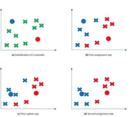
Figure 2.4 illustrates the first few steps of thek-Means algorithm on a small, two-dimensional data set. The green x’s are the data, and the blue and red circles are the cluster centroids. This
illustration begins with a random initialization of the two cluster centroids (seen in (a)). Next, the
firstassignment stepis executed (seen in (b)), thus each observation of data is assigned to the nearest centroid according to Euclidean distance. In this step, we update the color of each data observation
to indicate which cluster (red or blue) it has been assigned to. Next, the firstupdate stepis executed (seen in (c)). In this step the two centroids’ locations are updated to equal the mean of the data
that was assigned to it in the previous step. This step is analogous to those performed in lines
14 through 20 in the SOM algorithm (Algorithm 1) as it allows for the centroids to become better
Algorithm 2:k-Means Algorithm 1 Choose value ofk;
2 Initialize cluster centroidsc~j, for j=1, ..,k; 3 fort =1, ..,Tmax
4 fori=1, ..,D(each data vector in the data setSgiven byd~i)
5 Compute the index of the closest cluster centroid via:b(i) =argminjkd~i−c~jk2;
6 end
7 forj=1, ..,k
8 Bj=S(~b==j, :)(a matrix of all data vectors closest to cluster centroidj); 9 Letmj =Bj(the number of data vectors stored inBj);
10 Update cluster centroids:c~j =m1 j
Pmj
r=1Bj(r, :);
11 end
12 end
13 returnFinal cluster indicesb~ forSand final cluster centroidsc~j, for j=1, ..,k;
algorithm does not have an analog to the neighborhood update steps in the SOM algorithm (lines
22 through 27 in Algorithm 1) . The centroids ink-Means are neither aware of nor impacted by the location and training of each other, which is not the case in the SOM due to the implementation of a
neighborhood among the nodes. Lastly, we illustrate the beginning of the next iteration of training,
which begins again with anassignment step(seen in (d)). In this step, the data observations are compared to the locations of the updated centroids and reassigned to a cluster (red or blue) based
on their Euclidean proximity. Even by only considering this small example, we can recognize two
important features of thek-Means algorithm:
• the centroid initialization is highly influential in terms of how well the algorithm can perform
and how quickly it terminates, and
iteratively, based on the distances between the input data and all previously chosen centroids. By
considering the distances between a proposed centroid and the other centroids, thek++algorithm creates an initialization that is sufficiently spread out in the input data space and less likely to lead
to a poor clustering.
To address the second bullet, the choice ofkink-Means is somewhat analogous to the choice of the number of nodes (N) and their arrangement in the SOM algorithm. However, due to the lack of a neighborhood relation or connectivity among the centroids ink-Means, the algorithm will always produce a clustering with exactlyk clusters. Whereas in the SOM, the nodes in the map are connected via a neighborhood relation. Thus the position of a node is affected by both the data
assigned to it, and the data assigned to its neighbors. This feature allows for the algorithm to produce
(a)Initialization of 2 centroids (b)Firstassignment step
(c)Firstupdate step (d)Secondassignment step
2.3.1 Determining the Optimalk
When considering a two-dimensional data set for clustering, the natural first step would be to
generate a scatter plot of the data in order to get a sense of how many clusters we expect to observe.
However, as the dimension of the data set increases, visualization quickly becomes unfeasible. In
the case ofk-Means, it is the responsibility of the user to prescribe a value fork, i.e., we must first tell the algorithm how many clusters to look for. Without the ability to visualize the data, estimating
kbecomes a nontrivial, yet extremely important, task. To aid in this task, several methods have been developed. These methods rely on properties of the data set itself and a prescribedk to quantify the quality of a given clustering. Two of the most widely used methods are called the Elbow Method[31]
and the Average Silhouette Method[39].
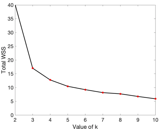
For the Elbow Method, we begin by choosing a range of possible integer values fork, for examplek= [2 : 10]. For each choice ofk, we randomly initializekcentroids, cluster the data, and compute the total within-cluster sum of squared distances (WSS) between the data observations
and their cluster centroid. The WSS is defined as
WSS= K X
k=1
X
i∈Dk
||xi−ck||22 (2.3)
whereDk is the set of data assigned to thek-th cluster,xi is thei-th data observation inDk, andck is thek-th cluster centroid. As the value ofk increases, the sum of squared distances will approach zero. However, this does not imply that a largek is inherently best. Consider the case where we letk equal the size of the data set,D. In this case, with careful centroid initialization, we expect the sum of squared distances to equal zero, since each data observation will form its own cluster. Clearly,
this is not optimal nor useful. Instead, we plot the WSS as a function ofkand look for the "elbow" in the graph to indicate an appropriate number of clusters. The "elbow" is defined as the point on the
graph at which the WSS, as a function ofk, begins to decrease linearly.
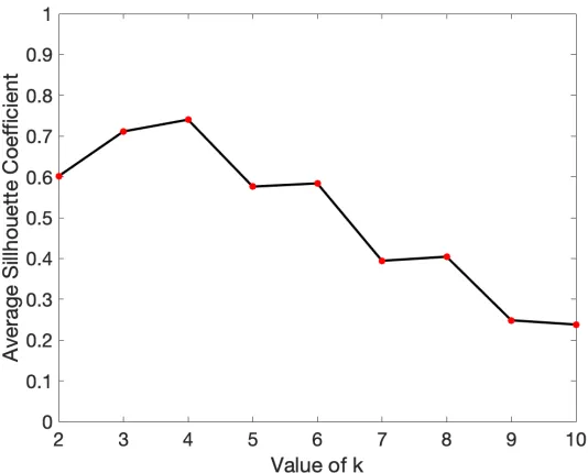
Similar to the Elbow Method, we begin the Average Silhouette Method by selecting a range of
observationxi is defined as
Si=
bi−ai max(ai,bi)
, fori=1, ..,D (2.4)
whereaiis the mean distance fromxito the other observations in the same cluster, andbiis the minimum mean distance fromxito observations in a different cluster. The silhouette coefficient is designed to measure the similarity of points assigned to the same cluster, and the average of the
silhouette coefficients across a clustered data set is used as the metric for assessing the quality of the
clustering overall[39]. The range ofSiis[−1, 1], with higher values indicating that a data observation is similar to other observations within its own cluster and dissimilar to observations in other clusters.
While the silhouette coefficient can be computed using any distance metric, we implement the
Euclidean distance throughout. We compare the average silhouette coefficients as a function of
the number of clusterskand choose the optimalkto be the one that produces the largest average silhouette coefficient.
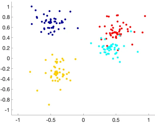
As a first illustrative example, we consider the two-dimensional data set depicted in Figure
2.5. The data set depicted in Figure 2.5 is generated from four known clusters. The observations in
each cluster are generated from a circular region about a prescribed centroid, with radii drawn from
the normal distributionr∼N(0, 0.22)and angular measure drawn from the uniform distribution
θ∼U(0, 2π). We apply both the Elbow Method and Average Silhouette Method to determine the
Figure 2.5Two-dimensional data set generated from 4 cluster distributions with radial varianceσ=0.22.