An Approach Of Features Extraction And Heatmaps Generation Based Upon Cnns And 3D Object Models

University of Windsor University of Windsor

Scholarship at UWindsor

Scholarship at UWindsor

Electronic Theses and Dissertations Theses, Dissertations, and Major Papers

9-27-2019

An Approach Of Features Extraction And Heatmaps Generation

An Approach Of Features Extraction And Heatmaps Generation

Based Upon Cnns And 3D Object Models

Based Upon Cnns And 3D Object Models

University of Windsor

Follow this and additional works at: https://scholar.uwindsor.ca/etd

Recommended Citation Recommended Citation

Pachika, Shivani, "An Approach Of Features Extraction And Heatmaps Generation Based Upon Cnns And 3D Object Models" (2019). Electronic Theses and Dissertations. 7830.

https://scholar.uwindsor.ca/etd/7830

This online database contains the full-text of PhD dissertations and Masters’ theses of University of Windsor students from 1954 forward. These documents are made available for personal study and research purposes only, in accordance with the Canadian Copyright Act and the Creative Commons license—CC BY-NC-ND (Attribution, Non-Commercial, No Derivative Works). Under this license, works must always be attributed to the copyright holder (original author), cannot be used for any commercial purposes, and may not be altered. Any other use would require the permission of the copyright holder. Students may inquire about withdrawing their dissertation and/or thesis from this database. For additional inquiries, please contact the repository administrator via email

AN APPROACH OF FEATURES EXTRACTION AND HEAT MAPS

GENERATION BASED UPON CNNS AND 3D OBJECT MODELS

By

Shivani Pachika

A Thesis

Submitted to the Faculty of Graduate Studies

through the School of Computer Science

in Partial Fulfillment of the Requirements for

the Degree of Master of Science

at the University of Windsor

Windsor, Ontario, Canada

2019

AN APPROACH OF FEATURES EXTRACTION AND HEAT MAPS

GENERATION BASED UPON CNNS AND 3D OBJECT MODELS

by

Shivani Pachika

APPROVED BY:

______________________________________________

M. Hlynka

Department of Mathematics and Statistics

______________________________________________

A. Ngom

School of Computer Science

______________________________________________

X. Yuan, Advisor

School of Computer Science

iii

DECLARATION OF ORIGINALITY

I hereby certify that I am the sole author of this thesis and that no part of this thesis has

been published or submitted for publication.

I certify that, to the best of my knowledge, my thesis does not infringe upon anyone’s

copyright nor violate any proprietary rights. Any ideas, techniques, quotations, or any other

material from the work of other people included in my thesis, published or otherwise, are

fully acknowledged in accordance with the standard referencing practices. Furthermore, to

the extent that I have included copyrighted material that surpasses the bounds of fair

dealing within the meaning of the Canada Copyright Act, I certify that I have obtained a

written permission from the copyright owner(s) to include such material(s) in my thesis

and have added copies of such copyright clearances to my appendix.

I also declare that this is an exact copy of my thesis, including any final revisions, as

approved by my thesis committee and the Graduate Studies office and that this thesis has

iv

ABSTRACT

v

DEDICATION

To the almighty God, my beloved parents Mr. Devender Reddy and Mrs. Jaya, my loving

vi

ACKNOWLEDGMENTS

I would like to take this opportunity to thank my supervisor Dr. Xiaobu Yuan for his

encouragement and support in presenting this thesis work. I have been extremely fortunate

to have a supervisor who has given me the freedom to explore things on my own, and with

his patient guidance whenever my steps faltered. His kindness and support have helped me

overcome many problems, throughout my project. It has been a great pleasure to work

under him as one of his research project students.

I would like to extend my gratitude to my thesis committee members Dr. Myron Hlynka

(Department of Mathematics and Statistics) and Dr. Alioune Ngom (School of Computer

Science) whose suggestions and recommendations significantly improved the quality of

this work. I would also like to thank them for spending their valuable time to assess the

thesis from my proposal to defense. I would also like to thank the secretaries of the

Computer science department, Mrs. Christine Weisener and Mrs. Melissa Robinet for all

the assistance, motivation and support given to me.

My special thanks goes to my friends and relatives for their constant encouragement and

love they provided to me at all times. I express my sincere appreciation for my fellow lab

vii

TABLE OF CONTENTS

Declaration of Originality………...iii

Abstract ……….………….………iv

Dedication ……….………….…….v

Acknowledgments……….……….……vi

List of Tables………...………x

List of Abbreviations/Symbols………...xi

List of Figures...……….xii

1 Introduction ……….….….….1

1.1

Overview...1

1.2

Sensing Technology comparison...………2

1.3

Problem Statement ...……….3

1.4

Motivation.………3

1.5

Thesis Contribution………...4

1.6 Structure of the thesis ……….…...4

2 Background Study………...………...5

2.1 3D model……….…………...5

2.2 Rendering………...…………5

2.3 Virtual 3D city model………...………...…...5

2.4 3D GIS………...6

2.5 Feature………...7

2.6 Feature Extraction……….………….……7

2.7 Feature Selection……….………...7

2.8 2D Feature Extraction Techniques……….…………8

viii

2.10 Computer vision tasks………....16

2.11 Object detection Algorithms……….……….18

2.11.1 Traditional methods.……….19

2.11.2 Deep learning methods……….20

2.12 Heat maps ……….….28

2.13 Annotations………....29

3 Literature Survey.……….30

3.1 Static object feature extraction techniques……….…...30

3.2 Dynamic object feature extraction techniques………...31

3.3 Static and Dynamic object feature extraction techniques…………...35

3.4 Static and Dynamic object detection techniques………...38

3.5 Related Works………..40

4 Proposed Methodology...43

4.1 Proposed Methodology

Overview ………...43

4.1.1 Training information ...44

4.2 Cars..………45

4.3 Buildings.……….48

4.4 Trees ………...……….……55

4.5 Traffic light....……….………….58

4.6 Working of the overall system...………...61

4.7 Working of the individual modules..………62

5 Implementation and Experiments.……….….66

5.1 Software and Hardware Requirements...………66

5.2 Cars……….….67

5.3 Buildings.……….71

5.4 Trees ………74

ix

6 Results and Evaluation...……….….78

6.1 Cars...78

6.2 Buildings and Trees……….………79

6.3 Performances Measures...81

6.4 Evaluations and Comparisons………..82

6.5 Advantages of proposed methodology.………....84

6.5.1 Advantage to dependency modules……….85

6.6 Limitations……….……….….85

7 Conclusion and Future Works……….86

7.1 Conclusion……….……….….86

7.2 Future Works ………...86

References/Bibliography……….87

Appendix ………..94

x

LIST OF TABLES

Table 1: Sensing Technology Comparison [49]……… 2

Table 2: List of tools used for implementation and experiments ... 66

Table 3: Suwajanakorn, S., et al. 2018 vs Our approach ... 82

Table 4: Comparison between different Keypoint Orientation formulae ... 83

xi

LIST OF ABBREVIATIONS/SYMBOLS

2D 2-dimensional

3D 3-dimensional

RGB Red Green Blue

OSM OpenStreetMap

XML Extensible Markup Language

GIS Geographic Information System

GPS Global Positioning System

LIDAR Light Detection and Ranging

SIFT Scale Invariant Feature Transform

SURF Speeded-Up Robust Feature

HOG Histogram of Oriented Gradients

FAST Features from Accelerated Segment Test

NMS Non-Maximal Suppression

BoF Bag-Of-Features

SVM Support Vector Machine

SSD Single-Shot Detector

ReLU Rectified Linear Units

RoI Region of Interest

CNN / ConvNet Convolutional Neural Network

FCN Fully Convolutional Network

R-CNN Regions based/with Convolutional Neural Networks

RPN Region Proposal Networks

R-FCN Region-based Fully Convolutional Networks

YOLO You Only Look Once

xii

LIST OF FIGURES

Figure 1: Google's self-driving car [69]……… 2

Figure 2: Uber’s autonomous car [11]………. 2

Figure 3: Views of the virtual 3D city model of Nancy [4]……….. 6

Figure 4: 3D-GIS [4]……… 6

Figure 5: Illustrative image local features (a) input image (b) corners (c) edges (d) regions [5]…. 7 Figure 6: Common 2D Feature Extraction Methods [6]……….. 8

Figure 7: Left: Input image and Right: Canny edge image [10]……….………… 10

Figure 8: Classification of popular corner detectors and descriptors [54]……… 12

Figure 9: 3D shape model rendered with different virtual cameras [72]……….. 15

Figure 10: Three most common computer vision tasks [1]………. 16

Figure 11: Steps for image classification using CNN [1] ... 17

Figure 12: Input and Output for object localization problems [1] ... 17

Figure 13: Multiple object detection and localization [1] ... 18

Figure 14: Illustration of HOG feature descriptors & SVM weights used for classification [74]… 20 Figure 15: CNN Architecture [1] ... 21

Figure 16: R-CNN Architecture [75] ... 22

Figure 17: FAST R-CNN Architecture [20] ... 23

Figure 18: SSD Architecture [1] ... 24

Figure 19: Faster RCNN Architecture [17] ... 25

Figure 20: Region Proposal Network (RPN) [17] ... 25

Figure 21: R-FCN Architecture [1] ... 26

Figure 22: Applying ROI onto the feature maps to output a 3*3 vote array ... 26

Figure 23: An illustration showing the effect of increasing the dilation of 3*3 filter [31] ... 27

Figure 24: Heatmap generated on a sample image [28] ... 29

Figure 25: Definition and Illustration of 20 selected vehicle key points [46] ... 32

Figure 26: Corresponding 3D model for each detection box is shown [47] ... 32

Figure 27: Motivation for multi-view vehicle re-ID [34] ... 33

Figure 28: Semi-automatic annotation process [34] ... 33

Figure 29: Defined 66 3D keypoints for car models [48] ... 34

Figure 30: Training pipeline for 3D car understanding [48] ... 34

Figure 31: The process of the algorithm [59] ... 35

Figure 32: Local Visual features are integrated into a feature vector by using BoF approach [61] ... 36

Figure 33: 3D shape search engine [62] ... 37

Figure 34: The learned CNN is applied to estimate the viewpoints of objects [35] ... 38

Figure 35: Illustration of YOLO [33] ... 39

Figure 36: System Architecture for Feature Extraction of car models ... 46

Figure 37: A circle of 16 pixels around the pixel under test [70] ... 49

xiii

Figure 39: System Architecture for Heatmap generation for buildings ... 53

Figure 40: System Architecture for 3D Tree reconstruction ... 56

Figure 41: The architecture of Faster RCNN [68] ... 57

Figure 42: Flowchart for traffic light detection ... 59

Figure 43: YOLO v3 Network Architecture [67] ... 60

Figure 44: Overall System ... 61

Figure 45: Pipeline for Creation of 3D virtual city ... 63

Figure 46: Static object elimination ... 64

Figure 47: Dynamic object recognition and identification ... 64

Figure 48: Virtual city update and dynamic object masking ... 65

Figure 49: Image Formation: Pinhole model (Perspective model) [66] ... 67

Figure 50: Training and Inference phase using Keypointnet [18] ... 68

Figure 51: Car feature extraction result ... 70

Figure 52: 16 pixels circle involved in the FAST algorithm[70] ... 71

Figure 53: Building feature extraction result ... 72

Figure 54: Building heatmap generation ... 74

Figure 55: Tree 3D reconstruction ... 75

Figure 56: Traffic light color detection module ... 77

Figure 57: epoch vs accuracy in car's training ... 78

Figure 58: epoch vs total loss in car's training ... 78

Figure 59: epoch vs mean_overlapping_bboxes ... 79

Figure 60: epoch vs class_accuracy ... 79

Figure 61: epoch vs loss_rpn_cls ... 80

Figure 62: epoch vs loss_rpn_regr ... 80

Figure 63: epoch vs current_loss ... 81

1

CHAPTER 1

INTRODUCTION

1.1Overview

A self-driving or autonomous vehicle can detect its environment and navigate without

human input. It can detect an environment using a range of methods, including cameras,

GPS and computer vision[2]. Automated driving is a rapidly advancing application area

with a complex structure and lots of progress in Deep Learning. Companies like Google,

Uber, Tesla, Mercedes and BMW have already released or foraying quick. The examples

of the self-driving vehicle are shown in Figure 1 and Figure 2.

According to recent outcomes of studies [36], feature extraction techniques are of critical

significance to many pattern recognition applications and systems involving detection,

recognition, registration, matching, reconstruction and classification. Object detection in

real complex environments is a challenging task for autonomous driving in the

aforementioned applications. A typical pipeline for object detection can be divided into

three stages: the selection of informative regions, extraction of features and classification.

Deep Learning has reformed Computer Vision and is the core innovation behind the

capabilities of a self-driving vehicle [1]. Convolutional Neural Networks (CNNs) are

pivotal to the improvement of object detection in this deep learning revolution.

We propose the integration of a new source of a priori information, the virtual 3D city

2

Figure 1: Google's self-driving car [69]

Figure 2: Uber’s autonomous car [11]

1.2 Sensing Technology Comparison

Table 1: Sensing Technology Comparison [49]

In consideration of all these differences shown in Table 1, autonomous vehicles can use a

camera because of its added advantages and with better machine vision, it can identify

3

1.3 Problem Statement

• In the real world, there are many associated risks and cost issues to acquire training

data for self-driving artificial intelligence algorithms.

• The dependence on 3D object models and their annotations, collected and owned

by individual companies is a hindrance to the development of the new algorithms.

• Their approaches remain fundamentally bounded by massive amounts of

human-annotated training data.

• This time-consuming process impedes the progress of these deep learning efforts.

1.4 Motivation

In recent years, exploration in the area of self-driving cars has increased. Nowadays,

outdoor positioning systems often rely on GPS because of its affordability and

convenience. However, GPS suffers from the occurrence of satellite masks especially in

urban environments, under bridges, tunnels or in forests. To provide continuous, accurate,

and high integrity position data, satellite-based localization systems should incorporate

additional sensors (as proprioceptive sensors or environment perception sensors) or

database (for example 2D digital map). Nevertheless, using only incremental encoders

placed on the rear wheels and gyroscopes is not sufficient in case of long GPS outages,

because the Dead-Reckoning (DR) localization is prone to drift error due to accumulation

of data. As an alternative, a new approach to back up the limitations of GPS and DR sensors

based localization is required. The proposed approach must aim at providing absolute

positioning information by integrating a virtual 3D city model and an on-board camera in

the localization process. If a GPS measurement is available, then this data is used to update

the prediction, else the 3D model/camera-based pose estimation corrects the prediction.

We can determine the vehicle pose by registering a priori virtual 3D city model with a

captured 2D image. These virtual environments can be purposefully and increasingly

challenging for critical applications, and will also be able to train a self-driving car to drive

4

variances before being placed on a real assembly line. In addition to the above, there is still

a visible gap between machine performance and that of humans’, inspiring and

recommending promising future bearings for the deployment of computer vision

applications.

1.5 Thesis Contribution

• The target of ongoing research is to present an approach that directly uses graphic

models from open source datasets as the virtual presentation of real-world objects

to develop new computer vision tasks related to self-driving vehicles.

• To train the system in a way that they can not only detect objects but also

differentiate with high accuracy.

• To train a network to extract features of 3D models for verification and elimination

of static and variable objects and identification of dynamic objects.

• Sensor and object recognition technologies for self-driving cars must fulfill

enhanced requirements in terms of accuracy, unambiguousness, robustness, space

demand and of course, costs.

1.6 Structure of the thesis

The overall structure of the thesis is organized in the following way: Chapter 2 begins with

the background study for feature extraction and object detection techniques. In Chapter 3,

literature survey and related works about feature extraction and object detection techniques

are discussed extensively. The proposed system is introduced in Chapter 4: the feature

extraction of cars and buildings, details of the overall system and connection of this thesis

work with the overall system are also discussed. In Chapter 5, we delve into details about

the implementation and experimental setup. Experimental results, detailed quantitative and

qualitative analysis are performed by comparing them with existing techniques are reported

5

CHAPTER 2

BACKGROUND STUDY

This chapter discusses the basic definitions and technical background of feature extraction

and object detection techniques.

2.1 3D Model

A 3D model is a three-dimensional object’s mathematical representation. Until it is

represented, a model is not technically a graphic model. A model can be represented

visually through a method called 3D rendering as a two-dimensional picture [3].

2.2 Rendering

The process of converting 3D wireframe models to 2D images automatically on a computer is called 3D rendering [3]. Advantages of 3D modeling over exclusively 2D methods include flexibility, ease of rendering, accurate photorealism, spatial reality, etc. Graphical

Models are dependent on the synergy between computer graphics, computer vision and

image processing. The traditional approach for generating virtual views of an object or a

scene is to render directly from an appropriately constructed 3D model.

2.3 Virtual 3D city model

The Virtual 3D city model is a realistic and accurate representation of the environment in

three dimensions. It is a geographically textured model of the surroundings where the

vehicle navigates as shown in Figure 3. Such virtual 3D city models are produced using

aerial/satellite imagery (photogrammetry), airborne laser scanner data (LIDAR), GIS and

3D computer graphic. There are different terms utilized for 3D city models in writing, for

6

need for 3D city models is growing and expanding rapidly in various fields, including urban

planning and design, architecture, environmental visualization and many more [4].

Figure 3: Views of the virtual 3D city model of Nancy [4]

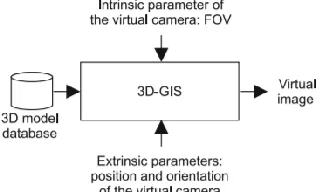
2.4 3D Geographical Information System

To manipulate the virtual 3D city model, we need to navigate effectively in the 3D model

by specifying the position and the orientation of theobserver in a chosen reference frame.

A computer tool has been developed for this purpose, referred to as the Three -

Dimensional Geographic Information System (3D-GIS). A 3D-GIS can conceptualize

terrain elevation, location of buildings, buildings facade texture, ground vegetation, rivers,

etc. The inputs of the 3D-GIS are the 3D model database and the desired calibration

parameters of the virtual camera. The 3D model database is composed of XML files

containing the tagged information of every place with geo-locations, height and area

information. The calibration parameters are the intrinsic parameters which are defined here

as the horizontal field of view (FOV) on the one hand and the extrinsic parameters on the

other. The latter being the position and the orientation of the virtual camera with respect to

the frame that is attached to the 3D model [4]. The design of 3D-GIS is shown below in

Figure 4.

7

2.5 Feature

A feature is described as “a piece of information which is relevant for solving the different

computational tasks related to a specific application” [54]. Feature points are also referred

to as keypoints/interest points/salient features. The idea of feature detection and description

refers to the process of identifying points in an image (interest points) that can be used to

describe the image’s contents such as edges, corners, ridges and blobs as shown below in

Figure 5. Features are categorized into two standard categories: local features and global

features. Local features are geometrical in shape, and global features are topological in

shape [5]. It is mainly aiming towards object detection, analysis and tracking from a video

stream to describe the semantics of its actions and behavior.

2.6 Feature Extraction

The term feature-detector (a.k.a extractor) traditionally refers to the algorithm or technique

that detects feature-points in an image. Subsequently, the recognized characteristics are

defined in logically distinct ways based on distinctive patterns that their adjacent pixels

possess. This method is called the feature description as it describes each feature by

assigning it a unique identity that allows for their efficient matching recognition. The terms

detector and extractor are used interchangeably in this work [5].

Figure 5: Illustrative image local features (a) input image (b) corners (c) edges (d) regions [5]

2.7 Feature Selection

Feature selection module is used for selecting a subset of relevant features from a large

8

contain better discriminatory power to help distinguish among different classes with better

accuracy. It also helps to reduce the dimensions of the feature space by selecting only the

distinguishable features [56].

2.8 2D Feature Extraction techniques

Several techniques have been created for feature extraction and their operating patterns are

quite distinct from each other as described in Figure 6. Each method’s performance is

optimal for a particular implementation.

Figure 6: Common 2D Feature Extraction Methods [6]

Different types of 2D traditional Feature Extraction techniques are:

Local Binary Patterns (LBP):

It is an optimal feature extraction technique for texture analysis. It divides the image

window into cells of 16 × 16 pixels, and every pixel in the cell is compared with eight of

its neighbors, in which the center pixel has a higher value than other pixels. After the cell

formation, a histogram is computed and normalized to make a feature vector. This feature

vector can be processed by machine learning algorithms or SVM for classification. The

improvements in LBP have enhanced the efficiency of face recognition applications, such

as over complete LBP, transition LBP, modified LBP, and RGB-LBP, which are enriched

with adjacent blocks overlapping, comparison of neighbor pixels, intensity values

9

channels, respectively. Another outstanding combination of HOG-LBP has proved that the

performance of LBP can be increased by combining it with other feature extraction

algorithms [6].

Color histogram:

A color histogram is the representation of the distribution of colors in a picture [9]. For

computerized pictures, a color histogram speaks to the number of pixels that have colors

in each of a settled list of color ranges that span the image’s color space, the set of all

conceivable colors. Color histograms are adaptable builds that can be built from pictures

in different color spaces, whether RGB or any other color space of any measurement. The

main disadvantage of histograms for classification is that the representation is dependent

on the object color, ignoring its shape and texture. Color histograms can be

indistinguishable for two pictures with distinctive protest substance which happens to share

color data. Then again, without spatial or shape data, comparative objects of diverse color

may be undefined based exclusively on color histogram comparisons [7].

Canny Edge Detection:

A well-known, general and robust approach for edge detection in digital images was

introduced by Canny. First, the input image is smoothed using a Gaussian filter.

Subsequently, the values of the first derivatives in the horizontal and vertical direction are

obtained by applying the Sobel operator to the smoothed input image. Using these values,

the gradient magnitude and the edge direction can be calculated. The resulting edges are

thinned using Non-Maximum Suppression (NMS). Subsequently, the remaining edge

pixels are classified using a high and a low threshold in the so-called hysteresis. Edges

above the high threshold are kept, edges below the low threshold are discarded. Edges

between the low and the high threshold are only kept if there is an edge pixel within the

respective 8-connected neighborhood [10]. This leads to a binary edge image as displayed

10

Figure 7: Left: Input image and Right: Canny edge image [10]

Structured Edge Detection (SED):

A more sophisticated, yet still real-time edge detection framework incorporating learning

and the use of information of the objects of interest has been proposed by Dollár and Zitnick

[71]. Therefore, in contrast to Canny edge detection, this approach requires a training

procedure using an annotated training corpus. Here, a Random Forest (RF)maps patches

of the input image I to output edge image patches using pixel-lookups and

pairwise-difference features of 13 (3 colors, 2 magnitudes, and 8 orientation) channels. While

testing, densely sampled, overlapping image patches are fed into the trained detector. The

edge patch outputs which refer to the same pixel are locally averaged. The resulting

intensity value (which lies in the interval [0,1]) can be seen as a confidence measure for

the current pixel belonging to an edge. Subsequently, an NMS can be applied to sharpen

the edges and reduce diffusion [10].

Scale Invariant Feature Transform (SIFT):

The SIFT method is used for extracting distinctive invariant features from images which

will be used to perform reliable matching between different images using a

nearest-neighbor algorithm. The significant steps in computation of SIFT are: 1) scale-space

extrema detection and keypoint localization based on Difference of Gaussian (DoG)

function to identify potential interest points; 2) orientation assignment to each keypoint

location based on local image gradient direction; 3) the keypoint descriptor measures the

11

Speeded-Up Robust Feature (SURF):

SURF is a local feature detection and matching method. The use of an integral image and

basic Hessian-matrix approximation has dramatically reduced the computational

complexity. The SURF parts consist of 1) interest point detection based on the Hessian

matrix that approximates second-order Gaussian derivative with box filters by using

integral images; 2) orientation assignment determined by constructing a circular region

around the detected interest point and the dominant orientation describes the orientation of

interest point; 3) interest point descriptors are built by extracting square windows around

the interest points and computing the Haar wavelet responses in horizontal and vertical

directions [8].

Histogram of Oriented Gradients (HOG):

Scale gradients, spatial binning, orientation binning, and contrast normalization are the key

steps for human detection using HOG. According to gamma normalization, different color

spaces that were used, such as LAB (LAB stands for Luminance/Lightness and A and B

are chromatic components) and RGB, and grayscale gamma normalization has reduced the

performance. This performance was evaluated by the false positive per window with

respect to the miss rate. Log compression was found to be weak compared to the square

root of gamma compression. Gaussian smoothing is used for gradient computation and

different scales are tested. In orientation binning, a weighted vote was calculated for each

pixel and these votes were summed up to make cells (orientation bins). The shape of cells

is of two types: rectangular and circular. These orientation bins were equally spaced as 0

degree to 180 degrees (unsigned) and 0 degree to 360 degrees (signed). Contrast

normalization and grouping blocks were performed for normalization. Two types of block

geometries have been introduced as rectangular and circular, which are known as R-HOG

12

Corner Detection Techniques

The term corner in detection does not mean to detect the physical corner such as the corner

of the table or chair, but these are points in images with high curvatures. Corner means a

point in the image whose gradient direction changes rapidly. The techniques of this class

select the portion of the image which possesses the distinct properties from their immediate

surroundings. Then, computes the key points or features which remain locally invariant or

constant. Using these features, the image can be detected in different scenarios: rotation,

scaling, translation and occlusion. Corner detection techniques are used for image

recognition, detection and analysis [55]. List of type of detectors and descriptors present in

Corner detection techniques are described in Figure 8 present below.

Figure 8: Classification of popular corner detectors and descriptors [54]

Forstner Corner Detector:

In 1986 Forstner presented a rotation-invariant corner identifier in light of the ratio between

the determinant and the trace of μ. The accuracy of sub-pixel is used to find the location of

a corner that is stable to a certain set of photometric and geometric transformations [54].

Harris Corner Detection:

Harris corner detection algorithm detects corners by forming a local search window and

13

algorithm identify peaks of low and high brightness levels. The center point of the window

detects the corner. The shifting process averages the variation in pixel intensity. When the

window is shifted along a flat or smooth part of the image where there is no drastic change

in the pixel intensities, no corners are detected. However, when there is no change in

intensity levels along the edge direction, an edge region is identified. When there is a

significant change in intensity level in every direction, a corner is recognized [27]. Harris

was successful in identifying robust features in any given image. But on account

that it was only detecting corners, his work suffered from a lack of connectivity of

feature-points which represented an essential obstacle for obtaining major level descriptors such

as surfaces and objects [7].

Shi and Tomasi (Min Eigen) Corner Detection:

Shi and Tomasi have proposed the modified version of the Harris corner detector. This

algorithm works in the almost same way like Harris but with a little change. Harris uses

corner selection criteria with the help of Response Function R, if the score of R greater

than a certain value, then the point will be called as a corner, where the score function

computed by using two Eigenvalues. Shi & Tomasi have used Eigenvalues to decide

corners instead of using score function [55]. It works quite well where even the Harris

corner detector fails. We consider a small window on the image then scan the whole image,

looking for corners. Shifting this small window in any direction would result in a large

change in appearance if that particular window happens to be located on a corner. Flat

regions will have no change in any direction. If there is an edge, then there will be no major

change along the edge direction [57].

2.9 3D Feature Extraction techniques

3D keypoint detection is a critical step of object recognition. Several 3D keypoint detectors

have been inspired by 2D feature engineering. The method for feature extraction should be

independent of data representation. The method also should be invariant under transforms

14

Different types of 3D Feature Extraction techniques are:

HOG 3D:

HOG3D is based upon histograms of oriented spatiotemporal gradients computed for a

space-time volume in the neighborhood of an interesting point. This volume is further

subdivided into video blocks. The gradient of each block is computed at different spatial

and temporal scales, using integral video representation. Then, regular polyhedrons are

used to uniformly quantize the orientation of the computed 3D gradients. The final gradient

vector for space-time volume is obtained by concatenating the gradient vectors of all

sub-blocks [58].

3D SIFT:

3D SIFT (Scale Invariant Feature Transform) extends the popular 2D SIFT to videos. The

authors use finite difference approximations to compute the magnitude and orientations of

3D gradients for space-time volume around the interest points. Orientations of 3D gradients

are parameterized by two angles: θ giving the gradient direction in 2D and φ encoding the

angle away from the 2D gradient. The gradient magnitude is quantified along uniform

orientations by dividing θ and φ into equally sized bins using meridians and parallels [58].

Harris 3D:

The Harris 3D detector is a space-time extension of the popular 2D (spatial) corner detector

known as the Harris detector. It is a spatiotemporal interest point detector. In order to find

spatiotemporal interest points, a second-moment matrix μ is computed for each video input

point (x,y,t), at different spatial (σ) and temporal (τ) scale values. It uses a separable

Gaussian smoothing function and space-time gradients. The descriptors used with Harris

3D are HOG/HOF descriptors. Harris3D might prove to be an inadequate representation of

video by giving only a sparse set of spatiotemporal interest points. To overcome this

limitation, dense sampling was introduced. Dense sampling extracts points at regular

15

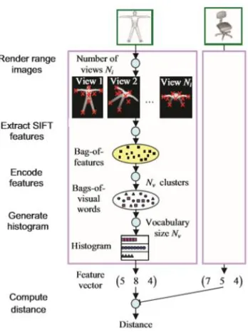
However, each 3D object can be represented by a set of multiple rendered views as shown

in Figure 9 instead of the original 3D model, some existing 2D image processing (feature

extraction) methods can be employed. These images are captured with a static camera or

virtual camera array [59].

Figure 9: 3D shape model rendered with different virtual cameras [72]

Ideal features should typically have the following essential qualities:

(1) Distinctiveness: The intensity patterns underlying the detected features should be rich

in variationsthat can be used for distinguishing features and matching them.

(2) Locality: Features should be local to reduce the chances of getting occluded as well as

to allow a simple estimation of geometric and photometric deformations between two

frames with different views.

(3) Quantity: The total number of detected features (i.e., features density) should be

sufficiently (not excessively) large to reflect the frame’s content in a compact form.

(4) Accuracy: Features detected should be located accurately concerning different scales,

shapes and pixels locations in a frame.

(5) Efficiency: Features should be efficiently identified in a short time to make them

16

(6) Repeatability: Given two frames of the same object (or scene) with different viewing

settings, a high percentage of the detected features from the overlapped visible part should

be found in both frames. Repeatability is greatly affected by the following two qualities.

(7) Invariance: In scenarios where large deformation is expected (scale, rotation, etc.), the

detector algorithm should model this deformation mathematically, as precisely as possible

so as to minimize its effect on the extracted features.

(8) Robustness: In scenarios where a small deformation is expected (noise, blur,

discretization effects, compression artifacts, etc.), it is often sufficient to make detection

algorithms less sensitive to such deformations (i.e., no drastic decrease in the accuracy)

[5].

2.10 Computer Vision tasks

Computer Vision is the interdisciplinary scientific field that can recognize and understand images and scenes. As depicted in Figure 10, the three most common tasks in computer

vision are the classification of an image, object classification with localization and object

detection.

Figure 10: Three most common computer vision tasks [1]

Classification of an image:

Image Classification is the most common computer vision problem where an algorithm

looks at a picture and classifies the object in it. Image classification has an extensive variety

17

medicine. Such problems are usually modeled using Convolutional Neural Nets (CNNs).

Figure 11 shows the high-level steps involved in a typical image classification task. The

input image is sent through multiple convolutional, pooling, non-linear layers and the

output of the final layer of the CNN is passed into a softmax layer which converts the

numbers between 0 and 1, giving the probability of the image being of a particular class.

Figure 11: Steps for image classification using CNN [1]

Object classification and localization:

Localization of object’s algorithms not only spots an object’s class but also it draws a

bounding box around an object’s picture position as displayed in Figure 12. To get the

bounding box location, four more numbers are added to the output layer. The final output

contains class labels and four numbers to locate the bounding box.

18

Multiple objects detection and localization:

If multiple objects are present in the image and the task is to detect them all, then that

would be a multiple object detection and localization problem. These kinds of issues need

to leverage the concepts learned from image classification as well as from object

localization. For the algorithm to detect all types of objects in an image, it needs to be

capable of classifying and localizing all the objects in the picture as shown in Figure 13.

This process is typically done using either a simple sliding window approach, wherein, the

cropped window is passed through a ConvNet (Convolutional Neural Network) and have the ConvNet make the predictions. The sliding window is passed through the entire image.

In the end, a set of cropped regions will remain, which will have some object, together with

the class name and its bounding box. This sliding window approach is a fundamental object

detection approach, and to tackle this problem, many advanced object detection algorithms

have been devised [1].

Figure 13: Multiple object detection and localization [1]

2.11 Object Detection Algorithms Overview

Object detection algorithms work by finding out the specific object by matching the

object’s pixel values and equating them with the particular picture frame. There have been

19

uses. These algorithms have progressed from binary classified based approach to a

learning-based approach [13].

2.11.1 Object Detection Traditional Methods

Viola-Jones Algorithm:

Viola-Jones algorithm was one of the breakthrough algorithms which was devised in 2001.

It was mainly used for face detection but also was applicable for the general-purpose object

detection techniques. It had four modules which included Haar Feature Selection, Integral

Image Creation, Adaboost Training and Cascade Classifiers.

The algorithm searches for various features in a face like eyes, nose, mouth, etc. and

computes face cascades and compares them with the Haar features to check for faces in an

image. Due to this purpose, for the face to be detected, the images needed to be properly

oriented with the face being frontal upright. This algorithm had very low false positives

and very high detection rates. However, the recognition of faces was not quite developed

as compared to detection rates, thus reducing practical implications [13].

Histograms of Oriented Gradients (HOG):

This algorithm interprets robust low-level features that are based on HOG. It is still

grounded upon the approach of hardcoded features like the Viola-Jones method, but it is

an alternative to exhaustive search. It initially converts to grayscale image and then finds

the object by pixel-by-pixel in a particular frame. It matches each pixel with its surrounding

pixels with reference to the intensity of darkness. By doing this, it can create a map of the

gradients of the pixel intensity variation. These gradients can assist us to locate the nuances

in an image. The HOG method computes the gradient orientation in localized portions of

the image to identify multiple objects in a particular image. To highlight the required parts

of the image and eliminate other background noise, feature descriptor can be used as

presented in Figure 14. An image (size width x height x channels) to a feature vector/array

20

The feature vector produced by the algorithm produces excellent results when fed to an

image classification algorithm like Support Vector Machine (SVM) [13].

Figure 14: Illustration of HOG feature descriptors and SVM weights used for classification [74]

2.11.2 Deep learning methods

Deep learning is a component of a broader family of machine learning methods based on

learning data representation [73]. Learning can be supervised, semi-supervised, or

unsupervised. Deep learning models can attain state-of-the-art accuracy, sometimes

surpassing performance at the human-level [15].

Deep learning architectures:

 Deep Neural Networks  Deep Belief Networks  Recurrent Neural Networks  Convolutional Neural Networks

CNN

The basic building blocks of ConvNets (or CNN) are the convolutional layers, max-pooling

or average pooling layers, and fully-connected layers. CNNs are connected as an

arrangement of interconnected layers. The layers are made up of repeated pieces of

convolutional, Rectified Linear Units (ReLU) and pooling layers. With a set of channels,

the convolutional layers convolve their input. The channels are naturally found within the

21

enables the network to memorize nonlinear combinations of the initial inputs, which is

called feature extraction. These learned features, also known as activations, from one layer,

become the inputs for the next layer. The pooling layers down-sample their inputs and help

consolidate local image features. Finally, the learned features become the inputs to the

classifier or the regression function at the end of the network. For image classification

problems, the last layer is a classifier, and for object localization problems, the last layer is

a combination of both [1]. The basic CNN architecture is represented in Figure 15.

However, it is difficult to locate items precisely by directly mixing CNN with a sliding

window approach. To address these issues, region-based CNN, that is, R-CNN, SPPnet and Fast-R-CNN have been proposed to improve object detection performance [17].

Figure 15: CNN Architecture [1]

R-CNN

R-CNN stands for Region-Based Convolution Neural Network and is a method that

depends on the external region proposal system. R-CNN has proved to show better

performance than other ensemble methods and feature types. R-CNN takes an input image

and extracts region proposals and computes rich features using large CNNs and then

classifies the image [13]. The basic R-CNN Architecture is shown in Figure 16. Although

R-CNN was the new state-of-the-art system for general object detection, it is tough to

identify small objects such as far-away cars and human faces, since the low resolution and

lack of contexts in each candidate box significantly decrease the classification accuracy in

them. Moreover, the two different phases in the R-CNN pipeline cannot be jointly

22

Figure 16: R-CNN Architecture [75]

FAST R-CNN

The main advantage of Fast R-CNN over previous state-of-the-art techniques lies in

multi-stage pipeline training. In terms of space and time, training is expensive in R-CNN. On

testing, it was observed that R-CNN based object detection was slow. R-CNN work is

slowed down because of the execution of a ConvNet forward pass for each object proposal

without sharing computation makes. The input image and a set of object proposals are fed

into Fast R-CNN. It first processes the image through various convolutional and pooling

layers and produces a convolutional map and then a fixed-length feature vector is extracted

from the feature map for each proposal Region of Interest (RoI). To output, the K object

classes by bounding boxes, each of these feature vectors are fed into a succession of fully

connected layers that [13]. The basic Fast R-CNN Architecture is shown in Figure 17. The

limitation of this approach is the prolonged computation time in the region proposal

generation step. Therefore, Fast R-CNN was further improved by Ren et al., 2015 and

Faster R-CNN was developed, which attained state-of-the-date object detection accuracy

23

Figure 17: FAST R-CNN Architecture [20]

Recent Approaches:

Recent advances in self-driving cars have prompted researchers to build a variety of object

detection algorithms. Most of these object detection algorithms are based on three

meta-architectures: Single Shot multi-box Detector (SSD), Faster R-CNN (Regions with

Convolutional Neural Networks) and Region-based Fully Convolutional Networks

(R-FCN). Each of these architectures fundamentally differs in the way they build their object

detection pipelines. A typical object detection pipeline can be mainly divided into three

stages: informative region selection, feature extraction, and classification [1].

Single-Shot Detector (SSD)

The term single shot means the tasks of object localization and classification are handled

in a single forward pass of the network. It is relevant to methods that require object

proposals because it encapsulates all computation in a single network by eliminating

proposal generation and subsequent pixel or feature resampling stages.

Based on a feed-forward convolutional network, a fixed-size group of bounding boxes and

their corresponding scores for the target classification instances are shaped by this

technique. Now by performing the non-maximum suppression step, the final detections are

shaped. For high-quality image classification (with their last classification layer removed),

the initial network layers are built on a standard architecture called as a base network (here

24

The SSD architecture builds on these base networks, by discarding the fully connected

layers and replacing them with a set of auxiliary convolutional layers. These additional

Convolutional layers enable the algorithm to progressively decrease the size of the input to

each subsequent layer and extract features at multiple scales [1].

Figure 18: SSD Architecture [1]

Faster R-CNN

It consists of two networks one for region proposal network (RPN) (as shown in Figure 20)

for generating region proposals and another for the network for detecting the object using

these proposals. The main difference between Fast R-CNN is that it uses a selective search

to create region proposals. As RPN shares the most computation with object detection, the

time cost of making region proposals is much smaller in RPN than selective search. The

region proposal network produces a cluster of boxes that are inspected by a classifier or a

regressor to check for the occurrence of objects. After RPN, we get different sizes of

proposed regions. Different sized regions mean different sized CNN feature maps. It’s

challenging to make an efficient structure to work on features of diverse sizes. A region of

Interest Pooling simplifies the problem by reducing the feature maps to the same size. A

fixed number of roughly equal regions (say k) are produced when an input feature map is

divided with ROI splitting, and then Max-Pooling is applied to it. Therefore, the output of

ROI Pooling is always k regardless of the size of the input. With the fixed ROI Pooling

outputs as inputs, lots of choices are available for the architecture of the final regressor and

25

Figure 19: Faster RCNN Architecture [17]

Figure 20: Region Proposal Network (RPN) [17]

Region-Based Fully Convolutional (R-FCN)

Region-based Fully convolutional networks introduced by Dai, J., et al. [75] provides an

accurate and efficient object detection. R-FCN closely resembles the architecture of Faster

R-CNN but instead of cropping features from the same layer where region proposals (RoI)

are predicted, crops are taken from the last layer of features prior to prediction. Dai et al.

argue this approach of pushing the cropping to the last layer greatly minimizes the amount

of per-region computation that must be performed. This paper states that the R-FCN model

(using Resnet 101) could achieve comparable accuracy to Faster R-CNN often at faster

26

Figure 21: R-FCN Architecture [1]

In R-FCN architecture above, a given input object is divided into feature maps each

detecting the corresponding region of the object. The feature maps are also known as

position-sensitive score maps. Taking the example of the 3 X 3 ROI in Figure 21 above,

we ask ourselves how likely each in the 3 X 3 matrix contains the corresponding part of

the object and assign a score to it. This process of mapping score maps and ROIs to the

vote array is called position-sensitive ROI-pool. The average of the resulting ROI pool

gives the class score for a given object in the given ROI [1], as shown in Figure 22 below.

27

Dilated CNN

The architecture of Dilated convolutions (à-trous convolutions/convolution with holes) is

based on the fact that dilated convolutions support the exponential expansion of the

receptive field without introducing additional parameters and sacrificing the resolution of

data at the output layer and computational cost and filling the vacant positions with zeros

to learn multi-scale features. In practice, no expanded filter is created instead, the

filter features (weights) are matched to distant (not adjacent) features in the input matrix.

The distance is determined via the dilation coefficient D. Generally, dilated convolutions

have improved performance. With dilated convolutions in different dilation rates, receptive

fields in various sizes can be obtained, those multi-scale features extracted are as displayed

in Figure 23.

One of the critical components of our design is the dilated convolutional layer. A 2-D

dilated convolution can be defined as follow:

y(m,n) is the output of dilated convolution from input x(m,n) and a filter w(i,j) with the

length and the width of M and N respectively. The parameter r is the dilation rate. If r = 1,

a dilated convolution turns into regular convolution.

In dilated convolution, a small-size kernel with k × k filter is enlarged to k + (k − 1)(r − 1)

with dilated stride r. Thus it allows flexible aggregation of the multi-scale contextual

information while keeping the resolution same [21]. They feature the scale of each

convolutional kernel that is (2l + 1) 2 where l is the dilation rate of this kernel [22].

28

In dilation1, there is a 1-pixel distance between each filtered pixel and its nearest neighbor.

In dilation2, there is a 2-pixel distance: the filter is only applied to pixels that are in both

odd-numbered rows and columns of each 5×5 region. In dilation3, the filter is applied to

only pixels in every third row and column of each 7×7 region, and so on.

These dilations allow for a model to perceive higher-order abstractions without the need

for dimensionality reduction. The main advantage of this type of mechanism is that the

model is capable of capturing the frequency component from the input signal. Using this

simple trick, the CNN can accommodate a larger receptive field also, thus letting the model

accommodate longer-range dependencies. The dilated convolution technique opens up the

possibility of making as many as required skips in the input data, so we have a better global

view of the problem domain, in our case, one-dimensional vibration signal. It can alleviate

the severe loss of spatial acuity due to multiple down samplings in a traditional deep

network [24]. Another added advantage is if one wants to replace multiple dilated

convolutional layers with a single convolutional layer with large size filter, it is safe. For

instance, two 3×3 filters with 2-dilation can be replaced by one 9×9 filter with 1-dilation

[25]. Dilated CNN can deliver 5×5 information with only nine weights instead of

conventional CNN, which needs 25 weights [26]. However, a key drawback of dilated

convolutions is exactly what they do not perform any subsampling, which is essential for

reducing the complexity of deep layers. Thus, models that use dilation still rely on regular

subsampling layers [23]. They are frequently used in model compression, audio

generation, semantic image segmentation, generic image classification, sound wave

synthesis, machine translation, signal processing, weakly-supervised object location, etc.

2.12 Heatmaps

Heatmap is a data matrix visualizing values in the cells by the use of a color gradient. This

gives a good overview of the largest and smallest values in the matrix. Rows and/or

columns of the matrix are often clustered so that users can interpret sets of rows or columns

29

In other words, a heatmap is a type of graphical representation of data that consists of a set

of cells, in which each cell is painted for a specific color according to a specific value

attributed to the cell. The term “heat” in this context is seen as a high concentration of

geographical objects in a particular place. Heatmaps show the distribution of objects or

phenomena across the entire surface. More generally, heatmaps can be viewed as the

surfaces of densities. Such surface density well illustrates the location of the concentration

of points or linear objects [37]. An example of a heatmap is shown below in Figure 24.

At a fundamental level, heatmaps are implemented as spatial matrices with cells colored

after their values. Explicitly, they encode a continuous quantitative variable as a color in

space through a color transfer function to a sequential color scheme [38].

Broadly speaking they fall into two classes: (i) image-based heat maps and (ii) data-matrix

heat maps. Image-based heat maps display numerical information that is mapped over an

image, an object or a geographic location. On the other hand, data-matrix heat maps display

numerical data in a pseudo-colored tabular or matrix format. The data may be subsequently

clustered using various measures of similarity or dissimilarity [39].

Figure 24: Heatmap generated on a sample image [28]

2.13 Annotations

From a technical point of view, annotations are usually seen as metadata, as they give

additional information about an existing piece of data. We do not need a server to create

local annotations. We can store annotation data in a local file system (local annotations -

can be seen only by their owner) or it can store annotations remotely, on annotations servers

30

CHAPTER 3

LITERATURE SURVEY

This chapter discusses the relevant background of recent works in the Feature Extraction

and Object Detection techniques

3.1 Static object feature extraction techniques:

Kaneva, B., et al. 2011 [30] proposed to use a photorealistic virtual world to gain complete and repeatable control of the environment to evaluate image features. They used two sets

of images rendered from the Virtual City and from the Statue of Liberty to evaluate the

performance of a selection of commonly-used feature descriptors, including SIFT, GLOH

(Gradient Location and Orientation Histogram), DAISY, HOG, and SSIM (the

Self-SIMilarity descriptor). They then used the virtual world to study the effects on descriptor

performance of controlled changes in illumination and camera viewpoint resulting in the

best performance of DAISY descriptor.

Cappelle, C., et al. 2012 [4] explored that in structured scenes, as indoor environments, line and edge are favored. But outdoor environments are often textured, so the usually used

features are points, corners. In their work, the chosen features are the well-known Harris

points. Once the Harris points are detected in the real image and in the virtual image, they

have matched these two sets of points.

The Li, H., et al. 2018 [51] elucidates that when the number of images is too large, or the time of image feature extraction is long, it is not conducive to the implementation of the

31

shortcomings of Harris corner detection, and proposes an algorithm based on adaptive

threshold Harris feature point selection is proposed. Firstly, the Harris algorithm is

optimized from the two aspects of adaptive threshold and prescreening feature points.

Then, in order to further reduce the pseudo-corner and prepare the image matching, the

Forstner operator is used to determine the best feature point.

In [29], the algorithms compared by author are Moravec, Susan, Harris, FAST, Eigen and

Forstner. The kinds of noise used are Gaussian, Poisson, salt & pepper and speckle. Results

of testing the accuracy of each corner detector on the image noise mentioned that; a) not

all corner detectors are able to find the corner points appropriately, b) all corner detectors

do not show the location of the corner of the point accurately, c) all the corner detectors

are very sensitive to all types of noise. The test results in this study show that the entire

corner detector is very sensitive to noise, in other words, the degree of accuracy of detection

results every corner detector will be strongly influenced by the noise and the type of noise

The commonly used key point descriptors like SIFT or SURF fail to obtain feature points

[M. Yamaguchi et al., 2017]. Recently, new approaches for feature extraction based on

deep learning methods [T. Faulhammer et al., 2016 and W. Kehl et al., 2016 and E.

Simo-Serra et al., 2015] have demonstrated excellent performance.

3.2 Dynamic object feature extraction techniques:

In this Wang, Z., et al. 2017 [46] paper, the author elaborates that with orientation invariant feature embedding, local region features of different orientations are calculated based on

20 keypoint locations as mentioned in Figure 25 and are well aligned and combined.

Firstly, vehicle images are propelled into the region proposal module, which produces the

response maps of 20 vehicle key points. The key point regressor takes the input image and

outputs one response map for each of the 20 key points. Instead of directly predicting

32

locations or some main vehicle components, e.g. the wheels, the lamps, the logos, the

rear-view mirrors, the license plates.

Figure 25: Definition and Illustration of 20 selected vehicle key points [46]

Chabot, F., et al. 2017 [47] goes on to explain that the Deep MANTA (Deep Many-Tasks),

architecture consisting of the robust convolutional network provides vehicle part

coordinates (even if these parts are hidden), part visibility and 3D template for each

detection. They use a 3D vehicle dataset composed of 3D meshes with real dimensions.

Several vertices are annotated for each 3D model. These 3D points correspond to vehicle

parts (such as wheels, headlights, etc.) and define a 3D shape for each 3D model. The main

idea of this approach is to recover the projection of these 3D points (2D shape) in the input

image for each detected vehicle. Then, the best corresponding 3D model for each detection

box is chosen as shown in Figure 26. For this purpose, they proposed a semiautomatic

annotation process using 3D models to generate labels on real images for the Deep

MANTA training. Labels from 3D models (geometry information, visibility, etc.) are

automatically projected onto real images providing a large training dataset without

labor-intensive annotation work.

33

Zhou, Y., et al. 2018 [34] states the possible reasons for the slow progress in Vehicle re-identification (re-ID) as the shortage of the special 3D structure of a vehicle and suitable

research data. Previous works have mostly fixated on some specific views (e.g., front) but

these methods are less effective in realistic situations, where vehicles usually appear in

arbitrary views to cameras as explained in Figure 27. In this paper, the author focused on

the uncertainty of vehicle viewpoint in re-ID, proposing two deep end-to-end architectures:

The Spatially Concatenated ConvNet (SCCN) and Convolutional Neural Network

(CNN)-LSTM Bi-Directional Loop (CLBL). Their models exploit the great advantages of the CNN

and long short-term memory (LSTM) to learn transformations across different viewpoints

of vehicles. Thus, a multi-view vehicle representation containing information about all

viewpoints can be inferred from the only one input view and then used to calculate distance

from learning. The output is presented in Figure 28. Experimental outcomes demonstrate

that their models have achieved consistent improvements over the state-of-the-art vehicle

re-ID approaches.

Figure 27: Motivation for multi-view vehicle re-ID [34]

34

To enable efficient labeling in 3D, Song, X., et al. 2019 [48] has built a pipeline by considering 2D-3D key point correspondences for a single instance and 3D relationship

among multiple instances.To efficiently annotate complete 3D object properties, they have

developed a context-aware 3D annotation pipeline. Nonetheless, KITTI only labels each

car by a rectangular bounding box and lacks fine-grained semantic key point labels (e.g.

window, headlight). In this paper, authors offer to the community the first large-scale and

fully 3D shape labeled dataset. Besides, they contributed the first large-scale database

suitable for 3D car instance understanding – ApolloCar3D, where each car is fitted with an

industry-grade 3D (Computer-Aided Design) CAD model with the absolute model size and

semantically labeled key points as presented in Figure 29.

Figure 29: Defined 66 3D keypoints for car models [48]

This dataset is above 20× larger than PASCAL3D+ and KITTI, the current state-of-the-art.

To enable efficient labeling in 3D, they build a pipeline by considering 2D-3D keypoint

correspondences for a single instance and 3D relationship among multiple instances as

pipelined in Figure 30. Complementing existing related datasets, we hope this new dataset

could serve as a long-standing benchmark facilitating future research on 3D pose and shape

recovery.