University of Windsor University of Windsor
Scholarship at UWindsor
Scholarship at UWindsor
Electronic Theses and Dissertations Theses, Dissertations, and Major Papers
2011
Gaussian Mixture Model based Spatial Information Concept for
Gaussian Mixture Model based Spatial Information Concept for
Image Segmentation
Image Segmentation
Thanh Nguyen
University of Windsor
Follow this and additional works at: https://scholar.uwindsor.ca/etd
Recommended Citation Recommended Citation
Nguyen, Thanh, "Gaussian Mixture Model based Spatial Information Concept for Image Segmentation" (2011). Electronic Theses and Dissertations. 438.
https://scholar.uwindsor.ca/etd/438
Gaussian Mixture Model based Spatial
Information Concept for Image Segmentation
by
Thanh Minh Nguyen A Dissertation
Submitted to the Faculty of Graduate Studies through Electrical and Computer Engineering in Partial Fulfillment of the Requirements for
the Degree of Doctor of Philosophy at the University of Windsor
Windsor, Ontario, Canada 2011
c
Author’s Declaration of
Originality
I hereby declare that I am the sole author of this thesis. I certify that, to the best of my knowledge, my thesis does not infringe upon anyone’s copyright nor violate any proprietary rights and that any ideas, techniques, quotations, or any other material from the work of other people included in my thesis, pub-lished or otherwise, are fully acknowledged in accordance with the standard referencing practices. Furthermore, to the extent that I have included copy-righted material that surpasses the bounds of fair dealing within the meaning of the Canada Copyright Act, I certify that I have obtained a written permis-sion from the copyright owner(s) to include such material(s) in my thesis and have included copies of such copyright clearances to my appendix.
Abstract
parameters in order to minimize the higher bound on the data negative log-likelihood, based on the gradient method. Experimental results obtained on noisy synthetic and real world grayscale images demonstrate the robustness, accuracy and effectiveness of the proposed model in image segmentation.
To my beloved Dad and Mom &
Acknowledgements
I am deeply indebted to my thesis advisor, Prof. Jonathan Wu, for his informed guidance, understanding, support and encouragement through the years. His depth and vision in this area are truly admirable, and he has been an inspira-tion to me in many ways.
I am grateful to my committee members Prof. Narayan Kar, Prof. Huapeng Wu, Prof. Dan Wu, and Prof. Peter X. Liu for reviewing my thesis and making many excellent suggestions to improve its substance and presen-tation. Their openness, encouragement and interest in my research were very important to me.
Thanks also go to Andria Ballo and Shelby Marchand from Department of Electrical and Computer Engineering for their reminders and assistance in various administrative tasks.
in our lab for encouragements and the joys and tears that we shared.
I thank my parents who always stand beside me. I could not complete this long journey without their never-ending love, support and prayer. I cannot find any word to express my deep appreciation to them. I just want to tell them how much I love them. I love you, Dad and Mom, and thanks for always being there for me.
Finally, I thank my best friend and beloved wife Dang Nguyen Thanh Yen, who always takes care of many things around me since I came here so that I could concentrate on this thesis. Her love has been a strong energy for my entire study.
This research has been supported in part by the Canada Research Chair Program, AUTO21 NCE, the NSERC Discovery grant, and OGS.
Thanh Minh Nguyen
The University of Windsor
Table of Contents
Author’s Declaration of Originality iii
Abstract iv
Dedication vi
Acknowledgements vii
List of Figures xiii
List of Tables xx
Symbols and Abbreviations xxi
1 Introduction 1
1.1 General Introduction . . . 1 1.2 Thesis Overview . . . 7
2 Standard Finite Mixture Model for Image Segmentation 10
2.1.1 The Gaussian Distribution . . . 10
2.1.2 The Student’s-t distribution . . . 12
2.2 Maximum likelihood for the Gaussian . . . 14
2.3 Standard Finite Mixture Model . . . 16
2.3.1 Gaussian Mixture Model . . . 16
2.3.2 Student’s-t Mixture Model . . . 19
2.4 The Expectation Maximization (EM) Algorithm . . . 22
2.4.1 EM Algorithm for the Gaussian Mixture Model . . . . 22
2.4.2 Relation between EM and K-means . . . 25
2.5 Gradient-Based Optimization Techniques . . . 27
2.6 Image Segmentation Evaluation . . . 30
2.7 Conclusions . . . 31
3 Gaussian Mixture Model based Markov Random Field 33 3.1 Introduction . . . 33
3.2 Gaussian Mixture Model based MRF for the Pixel Labels . . . 34
3.2.1 Markov Random Field Theory . . . 34
3.2.2 Hidden Markov models . . . 36
3.3 Gaussian Mixture Model based MRF for the Priors of the Pixel Labels . . . 39
3.4 Conclusions . . . 44
4.2 Proposed Method . . . 46
4.3 Parameter Learning . . . 50
4.4 Experiments . . . 52
4.4.1 Synthetic Images . . . 54
4.4.2 Natural Images . . . 58
4.5 Conclusions . . . 65
5 Fast and Robust Spatially Constrained Gaussian Mixture Model for Image Segmentation 66 5.1 Introduction . . . 66
5.2 Proposed Method . . . 70
5.3 Experiments . . . 74
5.3.1 Segmentation of Synthetic Images . . . 75
5.3.2 Segmentation of Grayscale Natural Images . . . 81
5.3.3 Segmentation of Colored Images . . . 83
5.4 Conclusions . . . 87
6 Conclusions 89 6.1 Summary of Main Contributions . . . 89
6.2 Future Directions . . . 91
References 94
Appendix A 110
List of Figures
2.1 Plot of the Gaussian distribution showing the meanµand stan-dard deviationσ. . . 11 2.2 Plot of Student’s-t distribution for µ = 0 and Λ = 1 for
vari-ous values of v. The limit v → ∞ corresponds to a Gaussian distribution with meanµ and precision Λ. . . 13 2.3 The graphical representation of a Gaussian mixture model for
a set of N pixel xi. . . 17
2.4 Synthetic image, (a): original image, (128x128 image) (b): Cor-rupted original image with Gaussian noise (0 mean, 0.02 vari-ance), (c): standard GMM. . . 18 2.5 Real world image (321x481 image resolution), (a): original
im-age, (b): Corrupted original image with Gaussian noise (0 mean, 0.02 variance), (c): standard GMM . . . 18 2.6 Synthetic image, (a): original image, (128x128 image) (b):
2.7 EM algorithm for the mixture of gaussians, (a): The original 2D point set with the initial condition, (b): Result of GMM with this initial condition. . . 24 3.1 Synthetic image, (a): original image, (b): Corrupted original
image with Gaussian noise (0 mean, 0.05 variance), (c): stan-dard GMM, (d): SIMF [63]. . . 38 3.2 Synthetic image, (a): original image, (b): Corrupted original
image with Gaussian noise (0 mean, 0.01 variance), (c): stan-dard GMM (time = 5.5s), (d): SVFMM [72] (time = 246.1s). . 43 4.1 The first experiment (128x128 image resolution), (a): original
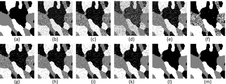
4.2 The second experiment (128x128 image resolution), (a): orig-inal image, (b): Corrupted origorig-inal image with mixed noise ( salt and pepper noise (0.03%) + Gaussian noise (0 mean, 0.01 variance)), (c): K-means (MCR = 24.609%), (d): standard GMM (MCR = 40.209%), (e): SVFMM (MCR = 22.338%), (f): ICM (MCR = 22.001%), (g): MODEF (MCR = 12.744%), (h): SIMF (MCR = 13.307%), (i): MEANF (MCR = 12.200%), (k) FGFCM (MCR = 5.562%), (l) HMRF-FCM (MCR = 3.692%), (m): The proposed method (MCR = 2.789%). . . 56 4.3 Affect of the simple competitive selection, (a): original image,
(b): Corrupted original image with Gaussian noise (0 mean, 0.03 variance), (c): MODEF (MCR = 3.512%), (d): MODEF with the simple competitive selection (MCR = 3.117%), (e): proposed method without the simple competitive selection (MCR = 0.199%), (f): proposed method with the simple competitive selection (MCR = 0.197%). . . 58 4.4 Images from the Berkeleys grayscale image segmentation dataset,
4.5 Image segmentation results obtained by employing the proposed method, (a): 135069, (b): 124084, (c): 58060, (d): 353013 with Gaussian noise (0 mean, 0.001 variance), (e): 239007, (f): 46076, (g): 15088 with Gaussian noise (0 mean, 0.005 variance), (h): 374067 with Gaussian noise (0 mean, 0.01 variance), (i): 302003 with Gaussian noise (0 mean, 0.01 variance). . . 60 4.6 Grayscale image segmentation (55067), (a): original image, (b):
K-means (PR = 0.879), (c): standard GMM (PR = 0.843), (d): SVFMM (PR = 0.882), (e): ICM (PR = 0.880), (f): MODEF (PR = 0.882), (g): MEANF (PR = 0.881), (h): FGFCM (PR = 0.879), (i): HMRF-FCM (PR = 0.887), (k): The proposed method (PR = 0.891). . . 62 4.7 Noisy grayscale image segmentation (24063), (a): original
im-age, (b): corrupted original image with Gaussian noise (0 mean, 0.005 variance), (c): K-means (PR = 0.778), (d): standard GMM (PR = 0.765), (e): SVFMM (PR = 0.787), (f): MODEF (PR = 0.814), (g): MEANF (PR = 0.818), (h): FGFCM (PR = 0.796), (i): HMRF-FCM (PR = 0.815), (k): The proposed method (PR = 0.826). . . 63 4.8 Computational cost (in seconds) comparison, (a): original
4.9 Minimization Progress of the negative log-likelihood function of the proposed algorithm, for the final experiment. . . 64 5.1 The first experiment (128x128 image resolution), (a):
origi-nal image, (b): Corrupted origiorigi-nal image with Gaussian noise (0 mean, 0.03 variance), (c): K-means, (d): Standard GMM (MCR = 41.67%), (e): SVFMM (MCR = 23.28%), (f): CA– SVFMM (MCR = 20.29%), (g): ICM (MCR = 20.23%), (h): SIMF (MCR = 3.83%), (i) MEANF (MCR = 3.55%), (j): Pro-posed method (MCR = 1.13%). . . 76 5.2 Maximization progress of the log-likelihood of the proposed
method of the first experiment. . . 77 5.3 The second experiment (128x128 image resolution), (a): original
5.4 The third experiment (128x128 image resolution), (a): original image, (b): Corrupted original image with Gaussian noise (0 mean, 0.03 variance), (c): K-means, (d): Standard GMM (MCR = 30.31%), (e): SVFMM (MCR = 18.11%), (f): CA-SVFMM (MCR = 17.73%), (g): ICM (MCR = 5.90%), (h): SIMF (MCR = 2.86%), (i) MEANF (MCR = 2.70%), (j): Proposed method (MCR = 0.21%). . . 80 5.5 The fourth experiment (256x256 image resolution), (a): original
image, (b): Corrupted original image with Gaussian noise (0 mean, 0.1 variance), (c): Proposed method in Chapter 4 (MCR = 0.10%, time = 8.9s), (j): Proposed method in Chapter 4 (MCR = 0.22%, time = 3.7s). . . 81 5.6 Grayscale natural image segmentation (80099), (a): original
im-age, (b): Standard GMM, (c): SVFMM, (d): CA–SVFMM, (e): SIMF, (f) MEANF, (g): Proposed method, (h): Maximization progress of the log-likelihood of the proposed method of this experiment. . . 82 5.7 Grayscale natural image segmentation (86016), (a): original
5.8 Grayscale natural image segmentation (374067), (a): original image, (b): Standard GMM, (c): SVFMM, (d): SIMF, (e): Proposed method. . . 84 5.9 Color image segmentation (310007), (a): original image, (b):
Standard GMM, (c): SVFMM, (d): CA–SVFMM, (e): SIMF, (f) MEANF, (g): Proposed method, (h): Maximization progress of the log-likelihood of the proposed method. . . 85 5.10 Color image segmentation (388016), (a): original image, (b):
Corrupted original image with Gaussian noise (0 mean, 0.0015 variance), (c): Standard GMM, (d): SVFMM, (e): CA–SVFMM, (f): ICM, (g) MEANF, (h): Proposed method. . . 86 5.11 (first row): original image, (second row): SVFMM, (third row):
List of Tables
4.1 Comparison of the proposed method with other methods in term of MCR (%), for the first experiment. . . 55 4.2 Comparison of the proposed method with other methods in term
of MCR (%), for the second experiment. . . 57 4.3 Comparison of image segmentation results on Berkeley’s grayscale
image segmentation dataset: Probabilistic Rand (PR) Index. . 61 5.1 Computational cost (in seconds) comparison for the synthetic
image in the first experiment. . . 76 5.2 Computational cost (in seconds) comparison for the synthetic
image in the second experiment. . . 79 5.3 Comparison of the proposed method with other methods in term
of MCR (%), for the third experiment, in the presence of varying levels of noise. . . 79 5.4 Comparison of image segmentation results on Berkeley’s color
Symbols and Abbreviations
xi : The i-th pixel of an image
N : The number of pixels in an image Ωj : The j-th label in an image
K : The number of labels in an image
Ni : The neighborhood pixels of the i-th pixel
Φ(xi|Θj) : The Gaussian function
µj : The mean of the Gaussian function Φ(xi|Θj) σj : The standard deviation of the Gaussian function
: Φ(xi|Θj), for the case of a single real-valued variable xi
Σj : The covariance of the Gaussian function Φ(xi|Θj),
: for the case of a D-dimensional vector xi
πj : The prior probability of all pixel belonging to the label Ωj πij : The prior probability of the pixel xi belonging
: to the label Ωj
zij : The posterior probability of the pixel xi belonging
f(xi|Π,Θ) : The density function at an observation xi p(X|Π,Θ) : The joint conditional density
L(Θ,Π|X) : The log-likelihood function
J(Θ,Π|X) : The negative log-likelihood function
H(Π,Θ|X) : The objective function
E(Θ,Π) : The error function GMM : Gaussian mixture model SMM : Student’s-t mixture model MRF : Markov random field EM : Expectation maximization
SVFMM : Spatially variant finite mixture model
CA-SVFMM : Class adaptive spatially variant finite mixture model NEM : Neighborhood expectation maximization
ICM : Iterated conditional model MODEF : Mode field algorithm SIMF : Simulated field algorithm MEANF : Mean field algorithm
FGFCM : Fast generalized fuzzy c-means
HMRF-FCM : Hidden Markov random field based fuzzy c-means MCR : The misclassification ratio
PR : The probabilistic rand index
Chapter 1
Introduction
1.1
General Introduction
In order to analyse the content of an image, it is often useful to construct a simpler representation of multiple segments. And the process to partition an image into non-overlapping regions that humans can easily separate is called image segmentation. In an image, various features can be used for segmen-tation process. These might be colour information that is used to create his-tograms, or information about the pixels that indicate boundaries or texture information.
environments, thereby increasing the productivity and profitability of automo-tive manufacturing enterprises and the global competiautomo-tiveness. In the field of medical imaging [4], [5], [6], [7], segmentation plays an important role. Accu-rate medical image segmentation provides additional information that helps to prepare treatment scheme and to evaluate therapeutic effect. The applications of segmentation vary from the detection of synthetic aperture radar images [8], [9], video analysis [10], to magnetic resonance imaging (MRI) [11], and object detection [12], [13], [14] etc. In all these areas, the quality of the segmented output affects on the quality of the final output largely. However, automated segmentation [15] is still a very challenging research topic, due to overlapping intensities and low contrast in images, as well as noise perturbation.
Many previous works have been proposed for image segmentation, in particular by the method of threshold [16], [17], [18]. However, thresholding is significantly susceptible to low resolution, low contrast and signal to noise ratio. As for some part of the image, high intensity variation may correspond to edges of interest, while the other part may require high low variation. The selection of the threshold is very crucial. A bad choice of threshold [19] leads to a poor quality of the segmentation. Adaptive thresholding [20], [21], [22] often is taken as a solution to this. However, it cannot eliminate the problem of threshold selection [23].
minimized the distance between the feature vectors. Although this approach worked well in the examples shown, it led to sub-optimal image segmentation. This is because the pixels in general are spatially correlated and the approach presented in this method did not incorporate any spatial information.
Many algorithms have been developed for image segmentation including graph-based methods [28], [29], mean shift based methods [30], [31], histogram-based methods [32], multi-scale segmentation [33], and clustering methods [34], [35], [36]. In clustering methods, K-means [37], [86] and fuzzy c-means [38] are two well-known methods that have been widely used for segmenting an image due to their simplicity and ease of implementation. However, one of their main drawbacks [39]–[42] is that these two methods ignore the spatial constraints in an image.
During the last decades, much attention has been given to model-based techniques [43], [44], [45], [100]–[105] to model the uncertainty in a probabilis-tic manner. In model-based techniques, standard Gaussian mixture model (GMM) [46]–[49] is a well-known method. It is a flexible and powerful sta-tistical modeling tool for multivariate data. Many researchers have used it to study a number of key problems in the area of image segmentation [50], [51]. In standard GMM, each pixel xi is considered to be a random variable whose
possibility density function Φ(xi|Θj) is a Gaussian function. The model
as-sumes a common prior distributionπj, which independently generates the pixel
given data set. The main advantage of the standard GMM is that it is easy to implement and requires a small number of parameters. The log-likelihood function that is used to estimate the parameters is inherently simple. How-ever, one of the main drawbacks of this model is that the prior distribution
πj has no dependence on the pixel index i. One of the other problems is that
the spatial relationships between the neighboring pixels are not taken into its account [58]. Although the standard GMM is a well known and simple method for image segmentation, its segmentation result is thus sensitive to noise, vary-ing illumination and other environmental factors such as wind, rain or camera shaking.
In order to reduce the segmentation sensitivity to noise, mixture models with Markov random field (MRF) have been employed for pixel labels [59], [62], [63], [64], [66]. The most important distinction is that in standard GMM, a common prior distribution πj for all pixels xi is evaluated, whereas, in these
approaches, the prior distributionπij varies for every pixel xi corresponding to
each label Ωj and depends on the neighboring pixels and their corresponding
parameters [67]. This prior distribution πij is a probability. Although these
approaches can lead to an improved segmentation quality, they lack enough robustness with respect to noise. In addition, the computational cost of the MRF based methods remains quite high.
pixel label, instead of the joint distribution of the pixel labels as in [59], [63], [64], [66]. These models work well for noisy image segmentation; however, in order to accurately evaluate the influence of the neighboring pixel labels during the learning step, the algorithm becomes complex and computationally expensive. In order to maximize the log-likelihood with respect to the param-eters in [58], [72], [73], the M-step of EM algorithm [58], [72] cannot be applied directly to the prior distribution πij. Therefore, various approximations have been introduced in order to tackle this problem. For example, the MAP algo-rithm in [58] cannot evaluate the prior distribution πij in a closed form, and
thus the gradient projection algorithm was proposed to implement the M-step. In [72], [73], another method based on a closed form update equation was used to implement the M-step, and estimate the parameters. As compared to stan-dard GMM based methods, the computational cost of these methods remains high. However, in addition to increased complexity, the final segmented image lacks adequate robustness to noise.
Based on these considerations, in the first part of this thesis, we pro-pose an extension of the standard GMM [82], [83] for image segmentation, which utilizes a novel approach to incorporate the spatial relationships between neighboring pixels into the standard GMM. The proposed model is similar to the standard GMM and thus easy to implement, with the main difference that the prior distribution of each label Ωj is different for each pixel xi and depends
require as many parameters as compared to the models based on MRF. To es-timate the unknown parameters of the pixel’s prior distributions, as well as the parameters of the distribution itself, instead of using the EM algorithm, we use the gradient method to minimize a higher bound on the data nega-tive log-likelihood. The proposed method has been applied for segmenting synthetic and real world grayscale images. The performance of the proposed model is compared with other methods based on standard GMM and MRF models, there by demonstrating its robustness, accuracy and effectiveness.
1.2
Thesis Overview
In the Chapter 2, the first group of model-based techniques is described begin-ning with the using of standard GMM to solve the fully unsupervised segmen-tation problem. The advantages and disadvantages of the standard GMM are then discussed. Next, in order to estimate the parameters of the model, vari-ous techniques based on maximizing their likelihood are described, beginning with the EM algorithm, then continuing with the gradient-based optimization techniques. The criteria evaluation for unsupervised segmentation algorithms is addressed before concluding with some observations regarding the relevance of the reviewed literature to the direction of research presented in our thesis.
most important distinction is that in standard GMM of the first group, a com-mon prior distribution for all pixels is evaluated, whereas, in the approaches of the second group, the prior distribution varies for every pixel corresponding to each label and depends on the neighboring pixels and their corresponding parameters.
Chapter 4 presents new unsupervised segmentation algorithms [82], [83]. In this chapter, we propose an extension of the standard GMM for image segmentation, which utilizes a novel approach to incorporate the spatial rela-tionships between neighboring pixels into the standard GMM. The proposed model is easy to implement and compared with MRF models, requires fewer parameters. We also propose a new method to estimate the model parameters in order to minimize the higher bound on the data negative log-likelihood, based on the gradient method. Results are presented before conclusions are drawn.
pro-posed method on many synthetic and real-world grayscale and colored images demonstrate its robustness, accuracy and effectiveness, as compared with other mixture models.
Chapter 2
Standard Finite Mixture Model
for Image Segmentation
2.1
Probability Distributions
2.1.1
The Gaussian Distribution
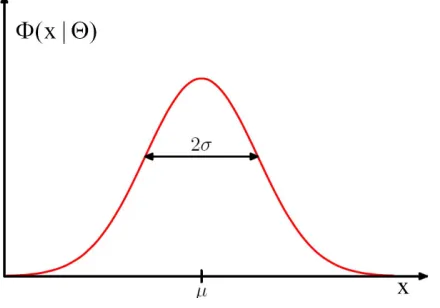
In probability theory, one of the most important distributions for continuous variables is Gaussian distribution. It is historically called the law of errors and is considered the most popular probability distribution in practice, and is used throughout statistics. For the case of a single real-valued variable x, the Gaussian distribution has its own mean µ and standard deviation σ and is defined by:
Φ(x|Θ) = √ 1
2πσ2 exp −
(x−µ)2 2σ2
!
Where Θ = {µ, σ}. The graph of the Gaussian distribution [80] is shown in Figure 2.1.
Figure 2.1: Plot of the Gaussian distribution showing the meanµand standard deviation σ.
As shown in Eq.(2.1), we see that the Gaussian distribution satisfies the two requirements for a valid probability density.
Φ(x|Θ) >0 (2.2) And,
∞
Z
−∞
Φ(x|Θ)dx = 1 (2.3) Within the Gaussian distribution defined by Eq.(2.1), the average value of x is
E[x] =
∞
Z
−∞
Φ(x|Θ)xdx =µ (2.4) And the variance of x is given by
varx2 =Ex2−E[x]2 =
∞
Z
−∞
For the case of a D-dimensional vector x, each Gaussian distribution Φ(x|Θ) can be written in the form:
Φ(x|Θ) = 1 (2π)D/2
1
|Σ|1/2 exp
−1
2(x−µ)
T
Σ−1(x−µ)
(2.6) where Θ = (µ,Σ). The D-dimensional vector µis the mean, the DxD matrix Σ is the covariance, and |Σ| denotes the determinant of Σ.
2.1.2
The Student’s-t distribution
Student’s-t distribution is a continuous probability distribution that is heavily tailed than Gaussian. Hence, it is more prone to producing values that fall far from its mean. Student’s-t distribution plays an important role in a number of widely used statistical analysis and is used to estimate the mean of a normally distributed population in situations where the sample size is small. It has proven to be quite effective for image segmentation [106].
Student’s-t distribution is symmetric and bell-shaped, like the normal distribution, meaning that it has its own parameters Θj ={µ,Λ, v}with mean µ, precision (inverse covariance) Λ and degree of freedom v. For the case of a
D-dimensional vector x, it has the probability density function.
S(x|Θ) = Γ(v/2 +D/2)|Λ|
1/2
Γ(v/2)(vπ)D/2
1 + ∆
2
v
−(v+D)/2
(2.7) where, Γ(·) is the Gamma function [80]:
Γ(y) =
∞
Z
0
and, ∆2 is the squared Mahalanobis distance from pixel x to meanµ.
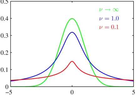
∆2 = (x−µ)TΛ(x−µ) (2.9) The degree of freedom v is illustrated in Figure 2.2. For the particular case of v = 1, the Student’s-t distribution reduces to the Cauchy distribution [80], while in the limit v → ∞ the Student’s-t distribution becomes a Gaussian with meanµ and precision Λ. Eq.(2.7) is the multivariate form of Student’s-t
Figure 2.2: Plot of Student’s-t distribution for µ = 0 and Λ = 1 for various values of v. The limit v → ∞ corresponds to a Gaussian distribution with mean µand precision Λ.
distribution and satisfies the following properties
E[x] =
∞
Z
−∞
S(x|Θ)xdx =µ (2.10) And the variance of x is given by
varx2=Ex2−E[x]2 =
∞
Z
−∞
S(x|Θ)x2dx−µ2 = v
v−2Λ
−1
2.2
Maximum likelihood for the Gaussian
Let xi denote an observation. Given a data set X = (x1,x2, ...,xN) in which
the observations xi are assumed to be drawn independently from a Gaussian
distribution, we can estimate the parameters of the Gaussian distribution by maximum likelihood [80]. The log-likelihood function is given by
L(Θ|X) = N D
2 log(2π)−
N
2 log|Σ| − 1 2
N
X
i=1
(xi−µ) 2
σ2 (2.12)
where Θ ={µ, σ}. After some manipulation, we see that the likelihood func-tion depends on the data set only through the two quantities
N
X
i=1
xi and N
X
i=1
x2i (2.13) The next objective is to optimize the parameter set Θ = {µ, σ} in order to maximize the log-likelihood function in Eq.(2.12). Let us now consider the derivation of the functionL(Θ|X) with the means µ, we have:
∂L(Θ|X)
∂µ =
N
X
i=1
xi−µ
σ2 (2.14)
and setting this derivative to zero, we obtain the solution for the maximum likelihood estimate of the mean at the (t+1) step. The mean of the observed set of data points is given by
µ(t+1) = 1
N N
X
i=1
xi (2.15)
with σ at the (t+1) iteration step, we have:
∂L(Θ|X)
∂σ = N X i=1 −1 σ +
(xi−µ)2 σ3
!
(2.16) The solution of ∂L(Θ|X)/∂σ = 0 yields the minimizer of σ at the (t+1) step. The result is as expected and takes the form
[σ2](t+1)= 1
N N
X
i=1
(xi−µ(t+1)) 2
(2.17) Note that the solution for µ(t+1) in Eq.(2.15) does not depend on σ(t+1), and so we can first evaluate µ(t+1) and then use this to evaluate σ(t+1). If we
evaluate the expectations of the maximum likelihood solutions under the true distribution in Eq.(2.15) and Eq.(2.17), we obtain the following results
Eµ(t+1) =µ (2.18)
and,
E
h
[σ2](t+1)i = N −1
N σ
2 (2.19)
As shown in Eq.(2.18), the expectation of the maximum likelihood estimate for the mean is equal to the true mean. However, the maximum likelihood estimate for the covariance has an expectation that is less than the true value. We can correct this bias by defining a different estimator [˜σ2](t+1) given by
[˜σ2](t+1) = 1
N−1
N
X
i=1
(xi−µ(t+1)) 2
2.3
Standard Finite Mixture Model
2.3.1
Gaussian Mixture Model
Over the last few years, much attention has been given to the standard GMM. An advantage of the standard GMM is that it requires a small amount of pa-rameters for learning. Another advantage is that these papa-rameters can be effi-ciently estimated by adopting the EM algorithm to maximize the log-likelihood function.
Let xi;i=1,2,...,N; denote the observation at thei-th pixel of an image.
Labels are denoted by Ω1,Ω1,...,ΩK. Consider the problem of estimating the
posterior probability of xi belonging to label Ωj. If we assume that xi is
drawn independently from the distribution, then the standard GMM [46], [75] assumes that the density function at an observation xi is given by:
f(xi|Π,Θ) = K
X
j=1
πjΦ(xi|Θj) (2.21)
The graphical representation of a Gaussian mixture model for a set of N
pixel xi is shown in Figure 2.3. Where Π = {π1, π2, ..., πK}, and πj is the
prior distribution of the pixel xi belonging to the label Ωj, which satisfies the
constraints:
0≤πj ≤1 and K
X
j=1
πj = 1 (2.22)
Each Gaussian distribution Φ(xi|Θj) is called a component of the
Figure 2.3: The graphical representation of a Gaussian mixture model for a set ofN pixel xi.
has its own mean µj and covariance σj and is defined by:
Φ(xi|Θj) =
1
q
2πσ2 j
exp −(xi −µj) 2
2σ2 j
!
(2.23) where Θj ={µj, σj}. The observation xiin Eq.(2.21) is modeled as statistically
independent. And the joint conditional density [58], [80] of the data set X = (x1,x2, ...,xN) can be modeled as:
p(X|Π,Θ) =
N
Y
i=1
f(xi|Π,Θ) = N Y i=1 " K X j=1
πjΦ(xi|Θj)
#
(2.24) Given the joint conditional density from Eq.(2.24), the log-likelihood function of the standard GMM [80] is given by:
L(Θ,Π|X) =
N X i=1 log ( K X j=1
πjΦ(xi|Θj)
)
Figure 2.4: Synthetic image, (a): original image, (128x128 image) (b): Cor-rupted original image with Gaussian noise (0 mean, 0.02 variance), (c): stan-dard GMM.
Figure 2.5: Real world image (321x481 image resolution), (a): original image, (b): Corrupted original image with Gaussian noise (0 mean, 0.02 variance), (c): standard GMM
Eq.(2.25), one of the biggest advantages of the standard GMM is that it has a simple form, and requires a small number of parameters.
However, the main drawback is that we cannot assign the same weight for every pixel belonging to the label Ωj, as the pixels in the image vary in
their intensity values and locations. Another limitation of the standard GMM is that the pixel xi is considered to be an independent sample. Therefore,
in Figure 2.4(b) into four labels. Figure 2.4(c) show the segmentation results for standard GMM. We can see that some details are lost in the segmented image. Another image from the Berkeleys image segmentation dataset [98], as shown in Figure 2.5(a), is used in next experiment. The image shown in Figure 2.5(b) is derived from the original image by corrupting it with Gaussian noise (0 mean, 0.02 variance). The objective is to segment the noisy image into two labels. As can be seen, the segmentation accuracy of standard GMM method, along the object boundaries is quite poor.
2.3.2
Student’s-t Mixture Model
To improve the robustness of the algorithm to outliers, Student’s-t distribu-tion has been used. The main advantage of the Student’s-t distribudistribu-tion is that it is heavily tailed than Gaussian, and hence finite mixture model of the longertailed multivariate Student’s-t distribution provides a much more robust approach to the standard GMM. It has proven to be quite effective for image segmentation [106]. In order to partition an image consisting ofN pixels into
K labels, standard Student’s-t mixture model (SMM) assumes that each pixel xi is independent of the label Ωj. The density function at a pixel xi is given
by:
f(xi|Π,Θ) = K
X
j=1
πjS(xi|Θj) (2.26)
where, Π = {πj}; j=(1,2,...,K); is the set of prior distributions modeling the probability that pixel xi is in label Ωj, which satisfies the constraints in
Each Student’s-t distribution S(xi|Θj), called a component of the
mix-ture, has its own parameters Θj = {µj,Λj, vj}. The Student’s-t distribution S(xi|Θj) is given by:
S(xi|Θj) =
Γ(vj/2 +D/2)|Λj|1/2
Γ(vj/2)(vjπ)D/2
1 + ∆
2 j vj
−(vj+D)/2
(2.27) where, Γ(·) is the Gamma function. And, ∆2 is the squared Mahalanobis distance from pixel xi to mean µj.
∆2 = (xi−µj)TΛj(xi−µj) (2.28)
The joint conditional density of the data set X = (x1,x2, ...,xN) is
mod-eled as:
p(X|Π,Θ) =
N
Y
i=1
f(xi|Π,Θ) = N Y i=1 K X j=1
πjS(xi|Θj) (2.29)
Then, the log-likelihood function of the standard SMM is given by the following identity:
L(Θ,Π|X) = logp(X|Π,Θ) =
N X i=1 log ( K X j=1
πjS(xi|Θj)
)
(2.30) Unfortunately, there is no closed form solution for maximizing the log-likelihood under a Student’s-t distribution. To overcome this problem, the Student’s-t distribution in previous SMM models [80] is represented as an infinite mixture of scaled Gaussians. In particular, we can write the Student’s-t distribution in the form.
S(xi|Θj) =
∞
Z
0
where, Φ(xi|µj, ujΛj) denotes the Gaussian distribution, and G(uj|vj/2, vj/2)
is the Gamma distribution. As apparent, the representation of the Student’s-t distribution as an infinite mixture of scaled Gaussians in Eq.(2.31) will corre-spond to an increase in complexity.
As shown from the log-likelihood function in Eq.(2.30), the pixel xi
in SMM is regarded as the same as xi in GMM. Each pixel xi is considered
independent of its neighbors. The spatial correlation between the neighboring pixels is not taken into account in the decision process. Moreover, the prior distributionπj does not depend on the pixel index and has the same value for
all pixels.
Figure 2.6: Synthetic image, (a): original image, (128x128 image) (b): Cor-rupted original image with Gaussian noise (0 mean, 0. 005 variance), (c): standard GMM, (c): standard SMM.
method, the standard SMM demonstrates a higher degree of robustness with respect to noise. However, as we see in Figure 2.6(d), the effect of noise on the result of standard SMM is still very high.
2.4
The Expectation Maximization (EM)
Al-gorithm
2.4.1
EM Algorithm for the Gaussian Mixture Model
In order to maximize the likelihood function given in Eq.(2.25), we need to determine the parameters of the GMM. Various techniques [48], [76] have been previously developed to determine these parameters, based on maximizing their likelihood L(Θ,Π|X) in Eq.(2.25), for a given data set. In [46], the well-known EM algorithm is used to approximate the maximum likelihood.
Let us begin by setting the derivatives of L(Θ,Π|X) in Eq.(2.25) with respect to the means µj of the Gaussian components to zero. We obtain
∂L(Θ,Π|X)
∂µj
=− N
X
i=1
πjΦ(xi|Θj) K
P
l=1
πlΦ(xi|Θl)
| {z }
zij
xi−µj σ2
j
= 0 (2.32) where we have made use of the form Eq.(2.23) for the Gaussian distribution. Note that the posterior probabilities zij appear naturally on the right-hand
side:
zij(t) = π
(t)
j Φ(xi|Θ (t) j ) K
P
l=1
πl(t)Φ(xi|Θ (t) l )
where t indicates the iteration step. The solution of ∂L(Θ,Π|X)/∂µj = 0
yields the minimum of µj at the (t+1) iteration step: µ(jt+1) =
N
P
i=1 zij(t)xi N
P
i=1 z(ijt)
(2.34) If we set the derivative ofL(Θ,Π|X) in Eq.(2.25) with respect toσj, and follow
a similar line of reasoning, we obtain [σj2](t+1)=
N
P
i=1
z(ijt)(xi−µ (t+1)
j )
2
N
P
i=1 zij(t)
(2.35) Finally, we maximizeL(Θ,Π|X) with respect to the prior distributionπj. Here we must take account of the constraint in Eq.(2.22), which requires the prior distribution πj to sum to one. This can be achieved by using a Lagrange
multiplierη and maximizing the following quantity:
∂ ∂πj
"
L(Θ,Π|X)−η K
X
j=1
πj−1
!#
= 0 (2.36) which gives
N
X
i=1
Φ(xi|Θj) K
P
l=1
πlΦ(xi|Θl)
−η = 0 (2.37) If we now multiply both sides by πj and use the constraint in Eq.(2.22), we
find η=N. Using this to eliminate η and rearranging we obtain
πj(t+1)= 1
N N
X
i=1
z(ijt) (2.38) We summarize the EM algorithm for Gaussian mixture model below:
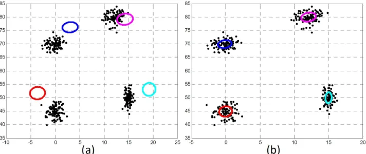
Figure 2.7: EM algorithm for the mixture of gaussians, (a): The original 2D point set with the initial condition, (b): Result of GMM with this initial condition.
covariance values σj and prior distributionsπj.
Step 2 (E-step): Evaluate the values zij in Eq.(2.33) using the current
pa-rameter values.
Step 3 (M-step): Re-estimate the parameters Ξ ={Θ,Π}={µj, σj, πj}.
+ Update the means µj by using Eq.(2.34).
+ Update covariance values σj by using Eq.(2.35).
+ Update prior distributionsπj by using Eq.(2.38).
Step 4: Evaluate the log-likelihoodL(Θ,Π|X) in Eq.(2.25) and check the con-vergence of either the log-likelihood function, or the parameter values. If the convergence criterion is not satisfied, then go to step 2.
After optimizing the parameters of the GMM and determining the posterior probability zij, Eq.(2.33) is used to assign labels to each pixel in the image.
four multivariate Gaussian distributions. Each component has one hundred data points. In Figure 2.7(a), we show the initial condition for EM algorithm. As shown in Figure 2.7(b), GMM is likely to successfully classify the data points.
2.4.2
Relation between EM and K-means
According to the K-means [86], each pixel xi in an image belongs to just one
label. It is based on the minimization of the following objective function:
H =
N
X
i=1 K
X
j=1
rij||xi−µj||2 (2.39)
The objective function in Eq.(2.39) represents the sum of the squares of the distances of each pixel to its assigned vector µj. The binary indicator variable rij is expressed as
rij =
1 if j = arg min
k ||xi−µk|| 2
0 otherwise
(2.40) The binary indicator variable rij in Eq.(2.40) describes which of theK labels
the pixel xi is assigned to. So that if data point xi is assigned to label Ωj
then rij=1, and rij=0 for j 6=k. In Eq.(2.39), the term ||xi−µj||2 expresses
the similarity between the data and the mean. The optimum is reached when the mean µj of the lable Ωj is found such that the objective function H in
Eq.(2.39) is minimized.
Now consider the optimization of the µj with the rij held fixed. The
H with respect to parametersµj is given by: ∂H
∂µj =−2 N
X
i=1
rij(xi−µj) (2.41)
The solution of ∂H/∂µj = 0 yields the minimum of µj at the (t+1) iteration
step:
µj = N
P
i=1 rijxi N
P
i=1 rij
(2.42) As an illustration in Eq.(2.42), we can see that one of the main advantages of K-means method is that it is very simple and easy to implement. Many researchers have used it in studying a number of key problems in image seg-mentation. However, from the objective function in Eq.(2.39), the pixel xi in
K-means is considered an independent sample, and thus this method does not take into account the spatial correlation between the neighboring pixels in the decision process. For that reason, the segmentation result of this method is very sensitive to noise.
Comparing the mathematical expressions of K-means with the EM al-gorithm for Gaussian mixtures, we see that there is a close similarity [79], [80]. As shown in Eq.(2.34), the EM algorithm makes a soft assignment based on the posterior probabilities zij. Whereas the K-means algorithm performs
a hard assignment of data points to clusters based on the binary indicator variables rij, in which each data point is associated uniquely with just one
Consider a Gaussian mixture in which the covariance matrices of the mixture components are given by εI, whereI is the identity matrix
Φ(xi|Θj) =
1
√
2πεexp
−||xi−µj|| 2
2ε
(2.43) Applying the EM algorithm in subsection 2.4.1, the posterior probabilities zij
for a particular data point xi, are given by zij =
πjexp{−||xi−µj||2/2ε} K
P
l=1
πlexp{−||xi−µl||2/2ε}
(2.44) If we consider the limit ε → 0, we see that zij → rij, where rij is defined
by Eq.(2.40). And the EM estimation equation for the mean µj, given by
Eq.(2.34), then reduces to the K-means result in Eq.(2.42). Note that the K-means algorithm only estimates the means but not the covariances of the labels. Finally, in the limit ε →0, the expected complete data log-likelihood [80], is given by
E[L(Θ,Π|X)]→
1 2
N
X
i=1 K
X
j=1
rij||xi−µj||2+ const (2.45)
From Eq.(2.45), we observe that K-means is a special case of the EM algorithm for Gaussian mixtures.
2.5
Gradient-Based Optimization Techniques
First of all, the prior probabilitiesπj corresponding to the label Ωj are chosen: πj =
exp(γj) K
P
k=1
exp(γk)
(2.46) The transformation given by Eq.(2.46) is called the softmax function, or nor-malized exponential, and ensures that, for −∞ ≤ γj ≤ ∞, the constraints in Eq.(2.22) are satisfied as required for probabilities.
Given the density function in Eq.(2.21) and the prior probabilitiesπj in
Eq.(2.46), we need to optimize the parameter set Ξ ={Θ,Π}={µj, σj, γj}in
order to maximize the log-likelihood function in Eq.(2.25). Since the logarithm is a monotonically increasing function, it is more convenient to consider the negative logarithm of the likelihood function [80], [82], [83] as an error function:
J(Θ,Π|X) =−L(Θ,Π|X) =− N X i=1 log ( K X j=1
πjΦ(xi|Θj)
)
(2.47) Applying the complete data [79], [80], [82], [83], minimizing the negative log-likelihood function in Eq.(2.47), is equivalent to minimizing the error function
E(Ξ(t)|Ξ(t+1)):
E(Ξ(t)|Ξ(t+1)) =− N X i=1 K X j=1
zij(t)log
n
π(ijt+1)Φ(xi|Θ(jt+1))
o
(2.48) where
zij(t) = π
(t)
j Φ(xi|Θ (t) j ) K
P
l=1
πl(t)Φ(xi|Θ (t) l )
To minimize this error function, we apply the gradient descent algorithm [79] to adjust the parameters Ξ = {Θ,Π} = {µj, σj, γj}. The change in the
parameters is then given by:
Ξnew= Ξold−η∇E(Ξold) (2.49)
where, ∇E(Ξ) = (∂E/∂µj, ∂E/∂σj, ∂E/∂γj), η is the learning rate and its
value is sufficiently small. The gradient of this error functionE(Ξ) with respect to parameters µj is given by:
∂E ∂µj =−
N
X
i=1
zij(t)xi−µj σ2
j
(2.50) Similarly, the derivative of E(Ξ) with respect to σj is given by
∂E ∂σj =− N X i=1
z(ijt) −1 σj
+(xi−µj)
2
σ3 j
!
(2.51) The derivative of E(Ξ) with respect toγj is expressed as:
∂E ∂γj =− N X i=1
z(ijt)−π(jt) (2.52) We summarize the gradient-based optimization techniques for Gaussian mix-ture model below:
Step 1: Initialize the parameters Ξ = {µj, σj, γj}: the means µj, covariance
values σj and the value ofγj.
Step 2: Evaluate the values zij in Eq.(2.33) using the current parameter
val-ues.
Step 3: Re-estimate the parameters Ξ ={µj, σj, γj} by using Eq.(2.49).
2.6
Image Segmentation Evaluation
Once the parameter-learning phase is complete, in order to assign labels to each pixel, the posterior probability zij is used. For each pixel xi, given the
posterior probabilityzij for all labels, in order to segment an image consisting
of N pixels into K labels, a determination is made, whereby the pixelxi is
assigned to the label with the largest posterior probability:
xi ∈Ωj : IFzij ≥zik; j, k = 1,2, ..., K (2.53)
In order to evaluate the segmentation performance quantitatively, the misclas-sification ratio (MCR) [91] is employed:
MCR = number of misclassfied pixels
total number ofpixels ×100 (2.54) The value of MCR is in the [0–100] range, where lower values indicate better segmentation results.
Another technique to obtain an objective performance evaluation is to adopt the probabilistic rand (PR) index [93]. For each image, the multiple ground truths are available and are denoted as G = {G1, G2, ..., GM}. The
segmentation map under evaluation is denoted as Geval. The PR index is
given by:
PR(G,Geval) =
2
M(M −1)
X
i
X
j>i
[cijpij + (1−cij)(1−pij)] (2.55)
where M is the number of image pixels. pij is the ground truth probability
The PR index takes a value in the interval [0–1]. A score of zero indicates a bad segmentation where every pixel pair in the test image has the opposite relationship as every pair in the ground truth segmentation. Otherwise, a score of one indicates a good result where every pixel pair in the test image has the same relationship as every pair in the ground truth segmentation.
In order to quantify the overlap between the segmented image and the ground truth for the label Ωj, the Dice similarity coefficient [94] is used:
Dicej =
2Vabj
(Vaj+Vbj)
×100 (2.56) Where,Vabj denotes the number of pixels that are assigned to label Ωj by both
the segmented image and ground truth. The number of pixels assigned to Ωj by the segmented image and the ground truth are denoted by Vaj and V
j b,
respectively. The Dice index attains the value in the [0–100] range, where higher values indicate better segmentation results.
2.7
Conclusions
Chapter 3
Gaussian Mixture Model based
Markov Random Field
3.1
Introduction
As mentioned in Chapter 2, a major shortcoming of standard GMM is that it does not take into account the spatial dependencies in the image. Moreover, it does not use the prior knowledge that adjacent pixels most likely belong to the same cluster. In this family of model-based techniques, prior probabilities [82] of label membership are considered constant for every pixel of an image. Thus, the performance of these methods is too sensitive to noise and image contrast levels.
labels are proposed in [59]–[64], [89], [90]. According to these approaches, prior probabilities are based on MRF to capture spatial information. The primary advantage of this family of mixture models is that it incorporates spatial infor-mation. Hence, it improves segmentation results, particularly when an image is corrupted by high levels of noise.
Another family of mixture models based on MRF for pixel label priors have been successfully applied to image segmentation [58], [72]–[74], [100]. Instead of imposing the smoothness constraint on the pixel label as in the above category, however, these methods aim to impose the smoothness constraint on the contextual mixing proportions. Their primary disadvantage, however, lies in its additional training complexity. The M-step of the EM algorithm in [72]– [74] cannot evaluate the prior distribution in a closed form, which therefore corresponds to an increase in the algorithm’s complexity. In [58] the gradient projection step was proposed to implement the M-step. Another reparatory projection step based on a closed form update equation was introduced [72] to guarantee that the prior probabilities are positive and sum to one.
3.2
Gaussian Mixture Model based MRF for
the Pixel Labels
3.2.1
Markov Random Field Theory
S, S = (1,2, ..., N), index a discrete set of N sites (pixels). And L, L = (1,2, ..., K) is a set of label. For every sitei∈ S, we consider a finite space Zi
of states zi, such as Zi = (zi,zi ∈ L). The space of the configurations of the
state values of the considered sites set is denoted by the product space.
Z =
N
Y
i=1
Zi (3.1)
Then, the p(Z) is a random field, if the following condition is satisfied
p(Z)>0, Z∈ Z (3.2) Now, let us denote the neighborhood of site i as Ni, i /∈ Ni and i ∈ Nj ⇔ j ∈ Ni. The neighborhood system on S is defined as N = (Ni, i ∈ S).
Then, the previously considered random field p(Z) is an MRF with respect to a neighborhood system N [91], [92] if and only if
p(zi|zS−{i}) =p(zi|zNi) (3.3)
Hammersley-Clifford theorem is proposed in [95], [96] to establish the equiv-alence of MRF and Gibbs random field. According to this theorem, a Gibbs distribution is equivalently characterized by a MRF and vice versa. Thus, an MRF given in Eq.(3.3) is rewritten as:
p(Z|β) =W−1exp (−U(Z|β)) (3.4) where, W is a normalizing constant called the partition function
W(β) = X
z∈Z
and U(Z|β) is an energy function. This energy function is a sum of clique potentials over all possible cliques of the form.
U(Z|β) =X
c∈C
Vc(Z|β) (3.6) Vc stands for the clique potential associated with the clique c. And C is a
label of subsets of the sites that contains sites that are all neighbors, and are known as cliques. β is a parameter of the clique potentials known as the inverse supercritical temperature. The computation of the termW in Eq.(3.5) involves all possible realizations Z of the MRF which is hardly ever feasible, in terms of computational requirements. To overcome this problem, an approximation of the likelihood in Eq.(3.4) is the pseudo-likelihood introduced by Besag [97] and defined as
p(Z|β) =
N
Y
j=1
p(zi|zNi;β) (3.7)
where, each term in the product is to compute
p(zi|zNi;β) =
exp (−P
ciVc(Z|β))
P
ziexp (−
P
ciVc(Z|β))
(3.8) The probability distribution in Eq.(3.8) is used to obtain estimates of a Markov random field parameters.
3.2.2
Hidden Markov models
Let us consider the problem of segmenting an image with N pixels, X = (x1,x2, ...,xN), intoK labels. In this model, the observations X are
label [59], [63], [64], [65], the density function at an observation xi is given by: f(xi|Π,Θ) =
K
X
j=1
πijΦ(xi|Θj) (3.9)
and the prior distributions πij are defined by:
πij =p(zi|zNi;β) (3.10)
where, the prior πij is different for each pixel i and depends on the neighbors
of the pixel. For more details, please refer to [64], [89]. Thus far, the problem has focused on how to estimate the parameters to maximize the following log-likelihood function:
L(Θ,Π|X) =
N X i=1 log ( K X j=1
πijΦ(xi|Θj)
)
(3.11) The iterative EM algorithm for estimating the parameters of the component densities is applied to estimate the parameters. The conditional expectation values zij of the hidden variables is computed as follows:
zij(t)= π
(t)
ij Φ(xi|Θ (t) j ) K
P
k=1
π(ikt)Φ(xi|Θ (t) k )
(3.12) The estimates of the means µj and covariance matrices Σj yield:
µ(jt+1) =
N
P
i=1 zij(t)xi N
P
i=1 z(ijt)
(3.13) and,
Σ(jt+1) =
N
P
i=1
zij(t)(xi−µj)(xi−µj)T N
P
i=1 zij(t)
Finally, the estimate of the inverse temperature parameter β yields
β(t+1) = arg max
β N
X
i=1 K
X
j=1
z(ijt)logp(zi =j|z (t)
N i;β) (3.15)
Figure 3.1: Synthetic image, (a): original image, (b): Corrupted original image with Gaussian noise (0 mean, 0.05 variance), (c): standard GMM, (d): SIMF [63].
3.3
Gaussian Mixture Model based MRF for
the Priors of the Pixel Labels
In order to reduce the sensitivity of the segmentation result with respect to noise, several researchers have suggested modifications to incorporate the local spatial interactions between the neighboring pixels. In the models in [58], [72]– [74]. the pixel label priors are treated as random variables forming an MRF have been presented in. In [58], the authors proposed a spatially variant finite mixture model (SVFMM) for image segmentation. The model assumes that the density function at an observation xi is given by:
f(xi|Π,Θ) = K
X
j=1
πijΦ(xi|Θj) (3.16)
where the Gaussian distribution Φ(xi|Θj) is the same as Eq.(2.23). The prior
distribution πij of the pixel xi belonging to the label Ωj should satisfy the
following constraints:
0≤πij ≤1 and K
X
j=1
πij = 1 (3.17)
Note that the observation xi in Eq.(3.16) is modeled as statistically
inde-pendent of the label Ωj. The joint conditional density [72] of the data set
X = (x1,x2, ...,xN) can be modeled as: p(X|Π,Θ) =
N
Y
i=1
f(xi|Π,Θ) = N
Y
i=1
" K X
j=1
πijΦ(xi|Θj)
#
(3.18) Since the observation xi is considered to be independent given the pixel label,
As a result, the segmented image is sensitive to noise, varying illumination and other environmental factors such as wind, rain or camera movements. To overcome this problem, MRF distribution [99] is applied to incorporate the spatial correlation amongst label values:
p(Π) =W−1exp
−1 TU(Π)
(3.19) where, W is a normalizing constant, T is a temperature constant. AndU(Π) is the smoothing prior. The posterior probability density function given by Bayes’ rules can be written as:
p(Π,Θ|X)∝p(X|Π,Θ)p(Π) (3.20) By incorporating Eq.(3.20), the log-likelihood function can be derived as:
L(Π,Θ|X) = log (p(Π,Θ|X)) = N X i=1 log ( K X j=1
πijΦ(xi|Θj)
)
+ logp(Π) = N X i=1 log ( K X j=1
πijΦ(xi|Θj)
)
−logW − 1 TU(Π)
(3.21) Depending on the type of energy U(Π) selected, we can have different kinds of models. In SVFMM method in [58], the value of T is set to one (T=1), and the Gibbs function for the priors p(Π) is given by:
p(Π) = 1
Z exp (−U(Π)) ; where : U(Π) = β N X i=1 K X j=1 X
m∈Ni
(πij −πmj) 2
where, Π is the parameter set; Π ={πij}; i=1,2,...,N; j=1,2,...,K. Andβ is a
scalar. The log-likelihood function (ignore the constant) is given by:
L(Π,Θ|X) =
N X i=1 log ( K X j=1
πijΦ(xi|Θj)
)
+ logp(Π) = N X i=1 log ( K X j=1
πijΦ(xi|Θj)
) −β N X i=1 K X j=1 X
m∈Ni
(πij −πmj) 2
(3.23) Compared to the log-likelihood function of the standard GMM in Eq.(2.25), the log-likelihood function in Eq.(3.23) is quite complex. In order to maximize this likelihood with respect to the parameters Ξ = {Θ,Π} = (µj,Σj, πij), an
iterative EM algorithm is adopted. Application of the complete data condition in [58], maximizing the log-likelihood functionL(Π,Θ|X) in Eq.(3.23) will lead to an increase in the value of the objective function H(Π,Θ|X).
H(Π,Θ|X) =
N X i=1 K X j=1
zij(t){logπij + log Φ(xi|Θj)} −β N X i=1 K X j=1 X
m∈Ni
(πij −πmj) 2
(3.24) where the conditional expectation values zij of the hidden variables can be computed as follows:
zij(t)= π
(t)
ij Φ(xi|Θ (t) j ) K
P
k=1
π(ikt)Φ(xi|Θ (t) k )
(3.25) Let us now consider the derivation of the functionH(Π,Θ|X) with the means
µj at the (t+1) iteration step. We have: ∂H
∂µj = N
X
i=1 zij(t)
−1
2(2Σ
−1
j µj −2Σ−j1xi)
The solution of ∂J/∂µj = 0 yields the minimizer of µj at the (t+1) step: µ(jt+1) =
N
P
i=1 zij(t)xi N
P
i=1 z(ijt)
(3.27) Thus, setting the derivative of the function in Eq.(3.24) with respect to Σ−j1 at the (t+1) iteration step we have:
∂H ∂Σ−j1 =
N
X
i=1 zij(t)
1 2Σj−
1
2(xi−µj)(xi−µj)
T
(3.28) and, equating it to zero yields:
Σ(jt+1) =
N
P
i=1
zij(t)(xi−µj)(xi−µj) T
N
P
i=1 zij(t)
(3.29) However, due to the complexity of the log-likelihood function in Eq.(3.23), the M-step of EM algorithm cannot evaluate the prior distribution πij in a closed
form. In order to maximize objective function H(Π,Θ|X) with respect πij
[58], [72], we set its derivative equal to zero and obtain the following quadratic expression:
4βNi
πij(t+1)2−4βπij(t+1) X m∈Ni
πmj −z (t)
ij = 0 (3.30)
where Ni stands for the set of neighbors falling in a window around the pixel
xi. The above equation has two roots: πij(t+1) =
P
m∈Ni
πmj ±
s
P
m∈Ni
πmj
2
+Ni
β z (t) ij
2Ni
(3.31) We select the root with the positive sign + since it yields πij ≥0. The above
πij of each pixeliat the M-step of every EM iteration. However, note that the
prior distribution πij should satisfy the constraints in Eq.(3.17). Therefore,
the algorithm becomes even more computationally complex. In [58], [72], [73], a large amount of computational power is utilized to solve the constrained optimization problem of the prior distribution πij.
To illustrate the computational cost of this approach, an image (245x245 image resolution) with three labels as shown in Figure 3.2(a) is used. The im-age shown in Figure 3.2(b) is made from the original imim-age by corrupting with Gaussian noise. All methods are initialized with the same initial condition and are performed on a PC (Core i3 with 4GB RAM) until convergence by using MATLAB in the Windows environment. As shown in Figure 3.2(d), al-though, SVFMM [72] demonstrates a higher degree of robustness with respect to noise, it is still low in terms of the speed. Note that SVFMM takes 246.1 seconds to segment this image. Compared to SVFMM, standard GMM is fast (5.5 seconds). However, the segmentation accuracy of standard GMM is quite poor as shown in Figure 3.2(c).
Another limitation of this model, as mentioned in [58], is that it requires a greater number of parameters compared to the standard GMM. In order to segment an image consisting of N pixels into K labels, we have to deal with
Kx(2+N) parameters (K parameters of µj, K parameters of Σj and N K
parameters of πij). This implies that the larger the image, the more the
number of parameters that we have to estimate.
3.4
Conclusions
In this chapter, mixture models based on the Markov random fields are pre-sented. Compared with the standards GMM, the major difference is that instead of using the common prior distribution πj for all pixels, the prior
dis-tribution πij of the mixture models based on the Markov random fields are
Chapter 4
An Extension of the Standard
Mixture Model for Image
Segmentation
4.1
Introduction
shaking.
In this chapter, we propose a new model based on the standard GMM that applies to the image classification problem. Our approach differs from those discussed above by the following statements. Firstly, a unique approach accounting for the relationship amongst neighboring pixels is presented. The proposed model is quite similar to the standard GMM and thus, is easy to implement. Secondly, compared to the standard GMM, the main difference in the proposed method is that the prior distribution πij of each label Ωj is
different for each pixel xi and depends on its neighboring pixels. Thirdly,
compared to the models based on MRF, the proposed model is simple and requires fewer parameters.
The rest of this chapter is organized as follows. In section 4.2, we describe the details of the proposed algorithm. Learning algorithms for the proposed system are presented in section 4.3. In section 4.4, we present the experimental results and conclude with a discussion in section 4.5.
4.2
Proposed Method
First, we define a function that represents the weight of each i-th pixel for each label Ωj.
ξj(xi) = exp −
(xi−cj) 2
2b2 j
!
(4.1) where cj and bj; j=1,2,...,K; are parameters whose optimal values can be
defined as:
ϑj(xi) =
" X
m∈Ni
exp −(xm−cj) 2
2b2 j
!#α
(4.2) where, α is a parameter, and Ni is the neighborhood of the i-th pixel (a
5x5 window is used in this method). Next, we propose a novel approach to incorporate the spatial relationships between neighboring pixels into the prior probability distribution πij. This prior distribution has different values for
each pixel corresponding to each label Ωj in the image, given by: πij =
ϑj(xi) K
P
k=1 ϑk(xi)
(4.3) The prior probability πij in Eq.(4.3) is computed subject to the constraints 0 ≤ πij ≤ 1 and PKj=1πij = 1. The density function at an observation xi is
given by:
f(xi|Π,Θ) = K
X
j=1
πijΦ(xi|Θj) (4.4)
The log-likelihood function is given by:
L(Θ,Π|X) =
N X i=1 log ( K X j=1
πijΦ(xi|Θj)
)
the MRF for πij, we propose a new way to incorporate the spatial
relation-ships between neighboring pixels into the prior distribution πij, as shown in
Eq.(4.3). Considering the formulae in Eq.(4.2) and Eq.(4.3), it can be easily seen that the prior distribution πij in the proposed method acts like a mean
filter. For that reason, the image segmentation result obtained by employing the proposed method is robust with respect to noise. We also propose a new method to estimate the model parameters in order to minimize the higher bound on the data negative log-likelihood [83], [82], [7], [77], [78], based on the gradient method that offers a closed form M-step, with computational complexity similar to that of the M-step for Gaussian mixture model.
The next objective is to optimize the parameter set Ξ = {Θ,Π} =
{µj, σj, cj, bj, α} to maximize the log-likelihood function in Eq.(4.5). Since
the logarithm is a monotonically increasing function, it is more convenient to consider the negative logarithm of the likelihood function [79], [80] as an error function:
J(Θ,Π|X) =−L(Θ,Π|X) =− N X i=1 log ( K X j=1
πijΦ(xi|Θj)
)
(4.6) Applying the complete data in [46], with proper replacements for old parameter (attiteration step) values with the new ones (att+1 iteration step) in Eq.(4.6), the change in the error function can be expressed as:
J(Θ(t+1),Π(t+1)|X)−J(Θ(t),Π(t)|X) =− N X i=1 log K P j=1
π(ijt+1)Φ(xi|Θ (t+1)
j )
K
P
k=1
π(ikt)Φ(xi|Θ (t) k )
× z (t) ij
zij(t)
Note, that zij(t), as shown in Eq.(2.33), always satisfies the conditions: zij(t)≥0 andPK
j=1z (t)
ij = 1. We can now apply the Jensen’s inequality [81] which states
that, given a set of numbers λj ≥0 and PKj=1λj = 1, we have:
log
K
X
j=1 λjyj
!
≥ K
X
j=1
λjlog (yj) (4.8)
From Eq.(4.8), the change in error function in Eq.(4.7) is given by:
J(Θ(t+1),Π(t+1)|X)−J(Θ(t),Π(t)|X)≤ − N X i=1 K X j=1
zij(t)log
π(ijt+1)Φ(xi|Θ (t+1)
j )
zij(t) K
P
k=1
πik(t)Φ(xi|Θ (t+1)
k ) (4.9) Thus, we have to minimize the log-likelihood function with respect to the new parameters (at the t+1 iteration step). Therefore, we can drop the terms that depend only on the old parameters (at the t iteration step). The change in the error function can be written in the form:
E(Θ(t),Π(t)|Θ(t+1),Π(t+1)) = − N X i=1 K X j=1
zij(t)lognπij(t+1)Φ(xi|Θ (t+1)
j )
o
(4.10) The E in Eq.(4.10) can be regarded as an error function. Therefore, max-imizing the likelihood L in Eq.(4.5) is then equivalent to minimizing E in Eq.(4.10). The minimization of the error function E with respect to the pa-rameters Ξ = {Θ,Π} = {µj, σj, cj, bj, α}; j=1,2,...,K; will be discussed in detail in the next part. In order to assign labels to each pixel, the posterior probability zij is used:
zij =
πijΦ(xi|Θj) K
P
k=1
πikΦ(xi|Θk)
After labeling each pixel using Eq.(4.11), a simple competitive selection is carried out for each pixel, in order to remove the remaining noise. If the i-th pixel belongs to labelj;j=1,2,...,K; and all its neighborhood pixelsNi belong
to the label k, k 6= j and k=1,2,...,K, then the i-th pixel is set to the label
k. It is worth noticing that we only use one type of selection criteria in this method: if all the neighbors of a given pixel are assigned to a specific label, the considered pixel is also assigned to the same label. The effect of this simple competitive selection employed in the proposed method is shown in the section containing the experimental results.
4.3
Parameter Learning
Thus far, the discussion has focused on probability estimation used to deter-mine the label Ωj to which the pixel xi should be assigned. To generalize
the posterior probability zij, we need to adjust the parameters Ξ = {Θ,Π}=
(µj, σj, cj, bj, α); j=1,2,...,K; to minimize the error function E in Eq.(4.10),
corresponding to maximizing log-likelihood functionLin Eq.(4.5). Note, that the total number of parameters required for the proposed method is only 4K+1 (K parameters of µj, K parameters of σj, K parameters of cj, K parameters
of bj and 1 parameter of α), which is less than the number of parameters in the models based on MRF mentioned in the section 3.3.
![Figure 3.1: Synthetic image, (a): original image, (b): Corrupted original imagewith Gaussian noise (0 mean, 0.05 variance), (c): standard GMM, (d): SIMF[63].](https://thumb-us.123doks.com/thumbv2/123dok_us/1446358.1177213/60.612.124.492.132.305/synthetic-original-corrupted-original-imagewith-gaussian-variance-standard.webp)
![Figure 3.2: Synthetic image, (a): original image, (b): Corrupted original imagewith Gaussian noise (0 mean, 0.01 variance), (c): standard GMM (time =5.5s), (d): SVFMM [72] (time = 246.1s).](https://thumb-us.123doks.com/thumbv2/123dok_us/1446358.1177213/65.612.127.488.505.607/synthetic-original-corrupted-original-imagewith-gaussian-variance-standard.webp)