ABSTRACT
PITTMAN, RANDALL BENJAMIN. Exploring Flexible Communications for Streamlining DNN Ensemble Training Pipelines. (Under the direction of Dr. Xipeng Shen.)
Parallel training of a Deep Neural Network (DNN) ensemble on a cluster of nodes is a common
practice to train multiple models in order to construct a model with higher prediction accuracy.
Existing ensemble training pipelines perform a great deal of redundant operations, resulting in
unnecessary CPU usage, or even poor pipeline performance. In order to remove these redundancies,
we need pipelines with more communication flexibility than existing DNN frameworks can provide.
This project investigates a series of designs to improve pipeline flexibility and adaptivity, while
also increasing performance. We implement our designs using Tensorflow with Horovod, and test
it using several large DNNs in a large scale GPU cluster, the Titan supercomputer at Oak Ridge
National Lab. Our results show that with the new flexible communication schemes, the CPU time
spent during training is reduced by 2-11X. Furthermore, our implementation can achieve up to 10X
speedups when CPU core limits are imposed. Our best pipeline also reduces the average power
© Copyright 2018 by Randall Benjamin Pittman
Exploring Flexible Communications for Streamlining DNN Ensemble Training Pipelines
by
Randall Benjamin Pittman
A thesis submitted to the Graduate Faculty of North Carolina State University
in partial fulfillment of the requirements for the Degree of
Master of Science
Computer Science
Raleigh, North Carolina
2018
APPROVED BY:
Dr. Guoliang Jin Dr. Hung-Wei Tseng
DEDICATION
ACKNOWLEDGEMENTS
I would like to thank my thesis advisor Dr. Shen for his unwavering assistance and encouragement
in the development of this project. I would also like to thank Dr. Seung-Hwan Lim at Oak Ridge
TABLE OF CONTENTS
List of Tables. . . vi
List of Figures. . . vii
Chapter 1 Introduction. . . 1
1.1 Background . . . 2
1.1.1 Deep Neural Networks . . . 2
1.1.2 Deep Neural Network Training Pipeline . . . 3
1.1.3 Heterogeneous GPU-CPU cluster for DNN training pipelines . . . 4
1.2 Overview . . . 5
1.2.1 Motivation . . . 6
1.2.2 Key Challenges . . . 7
1.2.3 Our Solution . . . 9
Chapter 2 Related Work . . . 11
2.1 Ensemble Learning . . . 11
2.2 Training Large DNNs on Distributed Systems . . . 12
2.3 Distributed Machine Learning Interfaces . . . 13
2.4 Storage Systems for DNN Training on Image Datasets . . . 14
Chapter 3 Ensemble Performance . . . 15
3.1 Duplicated Pipelines and the Implementation . . . 15
3.2 Settings for Testing . . . 16
3.2.1 Workloads . . . 16
3.2.2 Datasets . . . 16
3.3 Baseline . . . 17
3.3.1 Single Node . . . 17
3.3.2 Multiple Nodes . . . 20
Chapter 4 Optimized Pipelines . . . 22
4.1 Problem statement . . . 22
4.2 Horovod groups . . . 24
4.3 All-Shared . . . 25
4.4 Single-Broadcast . . . 26
4.5 Multi-Broadcast . . . 26
Chapter 5 Metrics for Evaluation . . . 28
5.1 Peak Preprocessor Throughput . . . 28
5.2 CPU Usage . . . 29
5.3 Core Usage Limits . . . 29
Chapter 6 Experiments and Results . . . 32
6.1 Methodology . . . 33
6.2 Peak Throughput . . . 35
6.3 CPU . . . 36
6.4 Energy Consumption . . . 38
6.5 Summary . . . 41
Chapter 7 Discussion . . . 42
7.1 Broader Description . . . 42
7.2 Future Work . . . 43
Chapter 8 Conclusion. . . 45
LIST OF TABLES
Table 3.1 Statistics comparing the total run time for 50 solo runs and a parallel run of 1000 nodes for 2000 Alexnet steps. . . 21
Table 5.1 Average core usage when using simulated 3 core allocation on a Titan node. . . 30
Table 6.1 Titan cluster specifications. . . 32 Table 6.2 Characteristics of the DNNs used in our tests. The layers and parameters data
was obtained from[19, 18, 34, 29]. The compute rate, in units of images-per-second, is our measurement of the rate at which each DNN can consume preprocessed data when using the specified batch size. . . 33 Table 6.3 Slowdowns under a 1-core limitation, measured relative to the 16-core
perfor-mance of the same DNN and pipeline. . . 38 Table 6.4 Jobs launched during an 8AM - 2PM reservation on one power metered cabinet
on Titan. Times are formatted ashh:mm:ss. . . 39 Table 6.5 The minimum energy usage for one of Titan’s metered cabinets, averaged over
45 minutes of idle time with 1-second interval sampling. . . 40 Table 6.6 Average energy consumption during training for each of AS and the baseline
LIST OF FIGURES
Figure 1.1 Shallow and deep networks are distinguished primarily by the number of hidden layers they contain. . . 2 Figure 1.2 A typical pipeline for DNN training. . . 3 Figure 1.3 Illustration of the inference stage of a DNN ensemble of size 3 for an image of
a sailboat. . . 6
Figure 3.1 For the default single pipeline, the preprocessing queue is always full, while the compute queue empties quickly. Thus the preprocessing task is the bot-tleneck. . . 18 Figure 3.2 Default single pipeline core utilization for each of the 16 cores on a single
Titan node when training Alexnet. The average core utilization over the entire graph is 94.3%. When the startup phase is excluded, the average is 96.0%. . . . 19 Figure 3.3 Duplicated pipelines that can be used to concurrently train DNNs. . . 20
Figure 4.1 Visualization of the MPI all-gather collective. . . 24 Figure 4.2 Illustration of the All-Shared (AS) pipeline. The datasetDis divided inton
partitions for each reader. . . 25 Figure 4.3 Illustration of the Single-Broadcast (SB) pipeline. The datasetDis divided
intop partitions for each reader instead ofn, since there are nowpreaders feeding their own preprocessor. . . 27 Figure 4.4 Illustration of the Multi-Broadcast (MB) pipeline. Similar to the Single-Broadcast
design, the dataset is divided intoppartitions. EachDifor 1≤i≤p is
broad-casted to all nodes with thei’th preprocessor node as the root. . . 27
Figure 6.1 Illustration of peak(n) for each pipeline. The number of preprocessors is changed between 5 and 20 when supported by the pipeline. The horizontal lines indicate the measured compute demand of a GPU on Titan. . . 34 Figure 6.2 CPU usage for SB and MB on Alexnet normalized to the CPU usage for AS. . . 35 Figure 6.3 CPU usage reduction for the All-Shared pipeline compared to the baseline.
Each network/ncombination was trained over 1000 steps. . . 36 Figure 6.4 Runtime improvement of AS over the baseline when CPU-core limits are
imposed. The ensemble contained 100 networks, each trained over 1000 steps. 37 Figure 6.5 Total power draw over entire cabinet reservation period. The 12 jobs run
during this time are described in Table 6.4. . . 39 Figure 6.6 Power draw comparison between AS and the baseline running 80 nodes of
Chapter
1
Introduction
The latest innovations in science and technology are being powered by Deep Learning. Virtually any
field that collects large amounts of data stands to benefit from this revolution. While the mathematics
behind neural networks has been known for decades, computing power has been insufficient to
materialize useful results. With the increased performance provided by hardware accelerators,
training Deep Neural Networks (DNNs) to learn datasets has become a viable option for industry.
Nevertheless, the most intelligent neural systems are still limited by the computing power of a
single device. The common resolution for this problem is to utilize many devices in parallel. Training
a group of DNNs over many devices is known asensembletraining. Therefore, the new question is
how to distribute the training task over many devices in a scalable manner. The issue with parallel
training is not in the power of each accelerator, but the rate at which data can be transferred between
them. A DNNpipelineis the set of tasks that moves data to the accelerator(s) for training. At present,
DNN pipelines can be a severe limitation on the potential performance and scalability of large
training tasks[17].
This work explores the benefits that optimized pipelines can provide for DNN ensemble training.
We will begin by demonstrating that standard ensemble pipelines can result in reduced training
performance, and also cause unnecessary CPU utilization. The root cause of these issues is the
input output hidden
(a) Shallow neural network with 1 hid-den layer.
input output
hidden 1 hidden 2 hidden 3
(b) Deep neural network with 3 hidden layers.
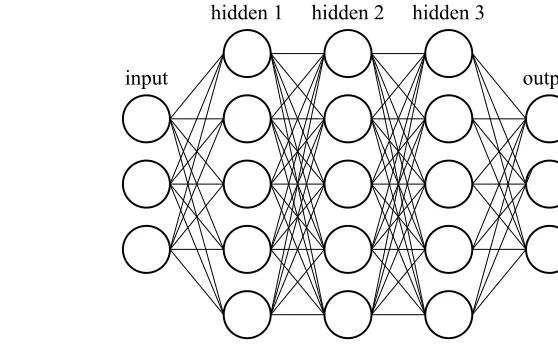
Figure 1.1: Shallow and deep networks are distinguished primarily by the number of hidden layers they contain.
various techniques that can be used to effectively eliminate these redundancies, allowing for far
more efficient ensemble training.
1.1
Background
1.1.1 Deep Neural Networks
Neural networks are often quantified in terms of the number oflayersthat make up the network.
This number is also the primary method of distinguishing betweenshallowanddeepnetworks (or
DNNs), as illustrated in Figure 1.1. Increasing the number of layers allows more complex datasets to
be represented, but also increases the computational complexity of training the network.
In recent years we have seen neural networks grow in size to accommodate demands for higher
accuracy and more complex datasets. This growth is due in part to the wide range of applications that
have been discovered for neural networks in nearly every field of study that gathers large quantities
1.1.2 Deep Neural Network Training Pipeline
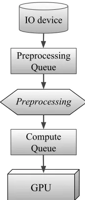
A typical deep neural network training pipeline contains three stages: reading the data from storage
systems, preprocessing the data, and training the model (see Figure 1.2). Data is first read into a
queue, and is then run through various transformations known as preprocessing. Afterwards, the
data is queued again and arranged intobatches. Thebatch sizeis the number of data the network
trains simultaneously per step. When training DNNs, it is important not to overfit to a particular
dataset. The goal of training is ultimately to adjust the weights to accept arbitrary elements of classes
that the input dataset is characterizing. Preprocessing typically helps with this goal by modifying
input data to be more generic.
Preprocessing Queue IO device
Preprocessing
Compute Queue
GPU
Figure 1.2: A typical pipeline for DNN training.
The standard preprocessing that is performed for most data is called “zero mean unit variance”,
which refers to the process of shifting and scaling input data to ideally approximate a normal
Gaussian distribution. Note that this process is performed collectively over the entire dataset, and
example, while maintaining the relationship between each data point.
Aside from such collective operations, many expensive data preprocessing operations are
per-formed on a point by point basis. For example, image preprocessing allows us to flip, rotate, blur,
and resize images to allow for more general cases than what is being provided by the dataset. While
this increases the computational complexity of the input pipeline, it also increases the generality
of the final DNN. Many other preprocessing techniques exist for other datatypes, not exclusively
images. Both audio[10]and sensor[13]data have a wide range of preprocessing techniques that
can be applied.
Preprocessing techniques can further be divided into online and offline preprocessing. In the
offline case, preprocessed data is saved to storage, then loaded directly into the pipeline when
training begins. This can help decrease the length of the pipeline and allow data to move directly to
the GPU for computation. Unfortunately, it also feeds the same data into the DNN when training
for multiple epochs1, thereby reducing generality. On the other hand, online preprocessing
tech-niques are used every time the dataset is loaded. Online is particularly useful when randomized
preprocessing techniques are used. Images may be flipped, rotated, or cropped in random ways,
allowing a single image to provide a vast array of possible inputs to a DNN. Online preprocessing is
the method commonly used in DNN training as its dynamic nature makes it more effective in
pre-venting overfitting a dataset, allowing much more general applications for the network. In modern
implementations of DNN training, online preprocessing typically serves as one stage in the training
pipeline; the pipeline structure helps hide its runtime overhead.
1.1.3 Heterogeneous GPU-CPU cluster for DNN training pipelines
The modern high performance computing cluster has evolved into a hybrid architecture that houses
CPUs and GPUs on each node in order to handle other computationally heavy workloads with high
energy efficiency[7, 36, 38]. One of the most prominent large-scale examples of such an architecture
is the Titan supercomputer located at Oak Ridge National Laboratory. Each of Titan’s 18,688 nodes
1An epoch is complete when the entire training dataset has been fed to the DNN once. DNNs are typically trained over
features both a 16-Core AMD CPU and a K20X Nvidia GPU[1]. The next supercomputer that will
soon be replacing Titan is called Summit, which is anticipated to be ready for researchers in 2018.
Summit will contain 2 IBM Power9 CPUs and 6 Nvidia Volta GPUs[2]. With this level of computing
power, researchers can use each node to either train larger networks, or train smaller networks faster
using techniques such as batch parallelism.
Heterogeneous GPU-CPU clusters are particularly well suited towards DNN training, since
the CPU and GPU can work together to accelerate the training pipeline. In heterogeneous
GPU-CPU clusters, the GPU is generally given the training task and the GPU-CPU is in charge of reading and
preprocessing data into batches that the GPU can quickly use, ideally with as little idle time as
possible. Such a division of pipeline steps is largely to achieve maximal training throughput on the
GPU, since GPUs are generally able to process machine learning kernels to train DNN models with a
higher throughput than multi-core CPUs[11]. To achieve maximal training throughput, it is generally
best to preserve cache and memory states on the GPU. If the GPU were to attempt preprocessing
as well as training, the CPU would need to perform additional copies to GPU memory depending
on how well the fusion of the preprocessing and training stages is performed. Furthermore, extra
memory would need to be allocated on the GPU for the preprocessing stage, which constricts the
maximum batch size that can be used on a large network. The general goal is to make the GPU’s
training stage as efficient as possible, while the preprocessing on the CPU side attempts to saturate
GPU resources.
1.2
Overview
Machine learning enables the discovery of actionable knowledge from large quantities of data.
In the training of machine learning models, including Deep Neural Networks (DNNs), machine
learning algorithms process a few samples of data in each training iteration for multiple iterations
to cover the entire data set until convergence[14]. As machine learning techniques evolve, more
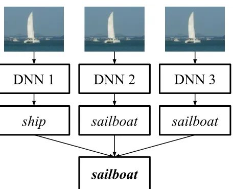
advanced usages have appeared such as theensembleof machine learning models[23, 14], where
DNN 1
DNN 2
DNN 3
ship
sailboat
sailboat
sailboat
Figure 1.3: Illustration of the inference stage of a DNN ensemble of size 3 for an image of a sailboat.
more accurate final prediction, as demonstrated in Figure 1.3. Such ensemble training multiplies the
I/O and CPU demand on an already burdened system, since it duplicates model training pipeline
across different nodes.
1.2.1 Motivation
The DNN training pipeline is an iterative process that consists of reading, preprocessing, and
computing/training stages. Data is first read from a storage system, then prepared for training using
the CPU, and lastly is sent to the GPU for DNN training. A common implementation of an ensemble
training pipeline is constructed by duplicating this pipeline onto multiple machines to train models
in parallel. Such a simple parallelization scheme inherently creates redundancies, particularly for
the preprocessing stage.
Since each DNN model is trained over the same data, the preprocessing operations (e.g., resizing
and cropping) being performed for each DNN are redundant. This stage can be CPU-intensive
depending on the type of operations being performed, the dataset being used, and the DNN model
to be trained. The result is unnecessarily high CPU usage for every compute node in the ensemble
side cannot keep up with the demand from the GPU to train a model over prepared data. In addition,
the excessive CPU usage is likely to increase the power consumption of the ensemble training.
Little work has been performed that relates directly to ensemble pipelines. Kurth et al.[20]is the
most closely related to this study, where the authors considered DNN training in high performance
computing environments. They focused on optimizing the communication of DNN model
param-eters, thereby allowing them to scale the training process to thousands of nodes. The study also
considered various communication methods in distributing training data, including preprocessing
and I/O from the storage systems, in the context ofmachine learning pipelines. However, this study
was performed on a cluster of Xeon-Phi processors, while our work uses a large scale GPU cluster.
While most of the related research focuses on training large DNNs, some has provided some
background on the problem of heavy preprocessing workloads. Microsoft researchers have produced
a tool called Adam[9]that is designed to scale large DNNs to potentially thousands of nodes. While
the tool primarily deals with accelerating larger networks over distributed nodes, their pipeline has
some elements in common with our current work. They mention concerns with heavy preprocessing
tasks caused by complex image transformations. They offload these tasks to a set of nodes dedicated
to queuing preprocessed data to feed worker nodes more efficiently. Such an allocation of work
requires extra nodes to perform the preprocessing. Our work does not use such a mechanism, but
instead distributes preprocessing only on the nodes that are being used to train DNNs. In this case,
no extra nodes are needed.
1.2.2 Key Challenges
The difficulty in resolving these redundant operations is the lack of flexibility in model training
pipelines. Since most present frameworks (e.g. TensorFlow, Caffe, and Torch) focus on training
a single model, they do not provide sufficient flexibility to allow pipelines to fit the demands of
parallelensemble training in distributed environments. The overarching goal of the research
di-rection presented here is to add flexibility into existing DNN frameworks to enable customizable
that best suit DNN ensembles in both training time and power consumption.
We can isolate four research challenges from this direction:
1. What part of the ensemble training process should be focused on?
2. How can we add flexibility into existing DNN training frameworks?
3. What pipeline designs fit the needs of ensemble training?
4. How can pipelines adapt to cluster hardware and DNN constraints to maximize performance
while minimizing cost?
Ensemble learning consists of reading, preprocessing, and training for each DNN. Which of
these stages presents the most performance issues that could be solved through a more intelligent
pipeline? We will analyze a series of queues used to buffer data between each of these stages, allowing
us to isolate potential bottlenecks. This will narrow down problems within the pipeline.
Present frameworks do not provide sufficient flexibility in pipeline design on distributed systems.
What additions can be made to current frameworks to allow for customizable and efficient pipeline
construction? In this work we focus on the Tensorflow framework, utilizing external libraries to
allow more adaptive and custom communication schemes.
With a flexible framework, what pipelines can we construct to remove computational
redun-dancies? We will examine 3 pipeline designs, and show that one of them in particular provides a
significant efficiency boost for ensemble training.
Beyond specific designs, is it possible to construct a pipeline that adapts to a particular
architec-ture, thereby providing optimal performance in any environment? What metrics for performance
should be used to establish the necessity of such a design? Such an analysis is beyond the scope of
this work, but here we provide a foundation for the optimization potential of this direction. In
par-ticular, we provide techniques that show the differences in scalability, performance, and efficiency
1.2.3 Our Solution
In this study, we analyze a series of queues used to buffer data between each stage in the machine
learning pipeline, allowing us to isolate potential bottlenecks. We discover a bottleneck in the
preprocessing stage that can hinder DNN training speed. To add flexibility to present frameworks,
we develop a group-based collective communication addition to the Horovod[27]library. Using
this addition with Tensorflow, we examine three pipeline designs that we refer to as All-Shared,
Single-Broadcast, and Multi-Broadcast.
The All-Shared pipeline shares the preprocessing step across all members in the ensemble,
whereas Broadcast and Multi-Broadcast share within a subset of the ensemble.
Single-Broadcast elects a leader to broadcast the preprocessed data to other nodes, while Multi-Single-Broadcast
performs asynchronous broadcasts from multiple nodes. We examine these three cases as an initial
study of different primitive pipeline communication schemes.
Among these pipelines, the All-Shared scheme provides significantly more efficient parallel
ensemble training. Our experimental results show that the preprocessing stage can indeed form
a bottleneck for the Alexnet DNN, producing 96% CPU usage with 34% degraded training time
on Titan supercomputer, a large scale GPU cluster at Oak Ridge National Lab. Our best optimized
pipeline can meet and exceed Alexnet’s preprocessing demand by up to 2X. We furthermore reduce
CPU usage by 2-11X depending on the DNN being trained. Lastly, we provide experimental results
on Titan showing that our best pipeline uses 5-16% less energy during training.
In summary, we present the following key contributions:
1. To our best knowledge, this is the first work that systematically characterizes performance
issues present in parallel DNN ensemble training in large distributed environments. (Chapter
3)
2. It adds to existing DNN ensemble training pipelines with flexible communication controls.
(Chapter 4)
parallel ensemble training pipelines in large distributed environments. (Chapter 4)
4. It offers a thorough performance analysis of the capabilities of these pipelines on the Titan
supercomputer. (Chapter 6)
We will first introduce DNN pipelines, showing how they can be extended for ensemble training.
After seeing the shortcomings of more simplistic designs, we will present our alternative pipelines.
Chapter
2
Related Work
This chapter introduces some of the ongoing work in the machine learning fields closely related
to distributed ensemble training. We will first look at some of the ensemble/multi-learner work
that has been proposed. Beyond this narrow scope is much research in training large DNNs on
clusters in a scalable manner. Towards this end, several machine learning APIs have been developed
to assist in automatically distributing the training process over cluster systems. There is also a push
to move more DNN training workloads from data-center clusters to theedgedevices in the Internet
of Things1. Researchers are thus developing neural network systems to train efficiently on low-end
CPU/GPU architectures. Lastly, we will cover some of the work related to storage systems for DNN
training on images, since our work uses the ImageNet dataset.
2.1
Ensemble Learning
Dr. Shiliang Sun’s research at East China Normal University has contributed several papers towards
the theoretical characteristics of ensemble learning (see[32],[33],[39], and most recently[40]). These
works survey the presently known mathematics behindmultiple-viewlearners. Such learners use
multiple views of the dataset to produce a neural network that is more generalizable and accurate.
1The Internet of Things (IoT) refers to the set of devices that can be connected together wirelessly, typically through
Both multi-view and ensemble learning attempt to alleviate the problem of overfitting a dataset
by introducing multiple intelligent systems, thereby making the overall system more generalizable.
However, multi-view learners look at the problem starting from the input data, while ensembles
introduce multiple learners on the same data. Sun et al. focus primarily on multi-view learning,
providing a thorough survey of previous work and present challenges in[40]. Our work looks at
ensemble learners when trained in parallel on distributed systems.
2.2
Training Large DNNs on Distributed Systems
In 2012 Google researchers (Dean et al.[12]) published a software framework calledDistBelief,
capable of utilizing compute clusters with possibly thousands of machines to train large DNN
models. They introduce some of the basic training algorithms needed to train such a large system
with reasonable scalability. The first technique they use isDownpour SGD, an asynchronous SGD2
model designed for a large number of model replicas3. They also use Sandblaster, a distributed
implementation of another popular training algorithm4. These two techniques are proposed as
mechanisms to share the changes in neurons within each DNN training device across the entire
cluster, a necessary step when training large DNNs on many devices.
In 2014 researchers moved towards using parameter servers as dedicated devices that stored
all the model’s variables, while the backpropagation task was sent to other worker devices. Li et
al.[21]in particular elaborate on this design, which is in some ways analogous to a master-worker
model for Deep Learning applications. Additionally, Microsoft researchers proposed project Adam,
a framework with similar goals to DistBelief which had been published 2 years earlier, but taking
the parameter server approach. In fact, project Adam has some similarities with our work. Since
they are training on the ImageNet dataset, they observe that preprocessing images quickly enough
is an expensive task. They solve this by delegating several nodes to work on preprocessing tasks to
2Stochastic Gradient Descent (SGD) is a common technique for training a neural network.
3DNNreplicasare copies of the same neural network on different devices. These are typically used to allow different
compute devices to calculate the gradients (an expensive operation) for the same DNN on different data in parallel.
4Specifically, L-BFGS, which is a limited memory implementation of the popular BFGS algorithm, where BFGS is
feed each model replica with data. Our work does not delegate extra nodes for this task, but instead
shares the preprocessing load between each CPU of the DNN trainers.
More recently, Chung et al. in 2017 published their work adapting a special DNN optimization
algorithm to the Blue Gene/Q cluster. This system is described as a large group of processors with fast
inter-processor communication. They illustrate how their algorithm is well-suited to Blue Gene/Q’s
architecture, and provide results demonstrating high scalability for large DNN training.
2.3
Distributed Machine Learning Interfaces
Many interfaces have been proposed for distributed machine learning over recent years. For example,
in 2013 Sparks et al.[31]presented MLI, an interface designed to help write machine learning
algorithms in a distributed setting. After the Tensorflow[5]framework began gaining traction
and popularity, several research groups introduced add-ons to Tensorflow that provided better
distributed capability. In 2017, MaTEx (Machine Learning Toolkit for Extreme Scale) was proposed
in[35]to add distributed memory capabilities to Tensorflow using MPI.
In a very recent work published in February of 2018, Sergeev et al. from Uber Technologies
introducedHorovod[28], another Tensorflow add-on. Horovod enables scalable DNN training
through its efficient GPU-based communication scheme that utilizes a ring-reduction technique
to average gradients over model replicas very quickly. Horovod has quickly gained popularity in
the research community for two reasons: (1) It is fast, using the latest known all-reduce techniques
with the NCCL library from Nvidia for faster GPU communication, and (2) it is incredibly simple to
install and use, requiring only a few lines of code to be modified.
In[28], the Horovod authors note that the concept of parameter servers had introduced
chal-lenges to researchers that made them more difficult to use. This technique required allocating some
number of nodes to be parameter servers, and the rest of the nodes to be workers. Such an allocation
is not straightforward in Tensorflow, and introduced an unpleasant learning curve for researchers.
Additionally, it is not necessarily clear how many servers should be allocated in the first place. Thus
and understand for users.
Our work uses Horovod for some of the MPI collective operations it supports, such as all-gather.
This enables us to present our work in terms of a pre-existing framework that is easy to use, without
unnecessarily developing a new distributed Deep Learning framework.
2.4
Storage Systems for DNN Training on Image Datasets
Image recognition is one of the more widely used applications for Deep Learning systems. With
the need for larger image datasets for more intelligent learners, storing these large datasets can
become a problem. Lim et al.[22]look at this problem for the ImageNet dataset using the Caffe deep
learning framework. They analyze the training rate of Alexnet when five different storage schemes
are applied, concluding that images cannot be stored individually, but must instead be allocated in
a dataset file system to improve performance (e.g. LMDB or LevelDB). Our work used the TFRecords
format to store the ImageNet dataset, since this was the technique recommended by Tensorflow.
Chapter
3
Ensemble Performance
In this chapter we discuss the scheme of the typical DNN ensemble training pipelines used in existing
work. We refer to such pipelines as theduplicated pipelinesscheme, and provide a Tensorflow
implementation that is used to test and analyze its performance. We later use this implementation
as a baseline against which other schemes may be compared.
3.1
Duplicated Pipelines and the Implementation
DNN ensemble training consists of the training of a number of DNN variants. These variants are
independent from one another. The scheme commonly used in existing work,duplicated pipeline
scheme, launchesN duplicated pipelines with each running on one (or more) nodes training one
DNN variant in the ensemble.
We implement the scheme based on Tensorflow.1We use the Slim module[4]as a starting point,
since it includes the implementations of several popular networks, such as Inception, Alexnet,
and VGG. Furthermore, Slim provides a robust set of preprocessing operations by default for the
ImageNet dataset, which proved quite useful for our tests. In our experiments, each DNN runs on
one Titan node.
3.2
Settings for Testing
We describe the settings used in our performance testing of various ensemble training schemes as
follows. Some of these choices are designed to draw out problems of interest that may arise from an
ensemble of DNNs.
3.2.1 Workloads
In general, parallel model training can be used as a fast method for hyper-parameter tuning[37],
or it can be used to create multiple learners for increased classification accuracy, or to learn an
ensemble model[23, 14]. An ensemble model is most effective when each DNN serves a useful and
probably unique testing purpose, and has been modified appropriately to suit that purpose. As
discussed earlier, the final result is intended to be more diverse than any single classifier could be.
Towards this goal, our study investigates the system efficiency of parallel ensemble training.
The more complicated case arises when the differences between each DNN are substantial
enough to causesignificantchanges in performance. For example, each model may contain varying
numbers of hidden layers or different numbers of nodes within each layer. Since the number of
layers in a network is a primary factor influencing training time[14], such changes could cause
significant differences in training times between the members of the ensemble. While this area
may be an interesting point for a future optimization study, managing the burst computational
requirements from many concurrent model training pipelines poses the most urgent problem.
In light of this, our experiments focus on the DNN variants in an ensemble that are of the same
structure but differ in their learning rates, initial filter values, or other non-structural parameters.
3.2.2 Datasets
When considering the effects of preprocessing, computation, IO usage, network traffic, etc., it is
reasonable to require that the input dataset dimension and the number of elements be large. Smaller
datasets such as MNIST or Cifar-102will likely require very little resources and will train quickly.
The primary dataset used for this research is a subset3ofImageNet[26], where the entire dataset
contains over 14 million images of size 224×224. With this dataset it is much easier to investigate the performance effects of DNN ensembles. For a given dataset, we also expect that every image
will need to be processed by every DNN in an ensemble.
3.3
Baseline
In this section we provide data that characterizes the performance of individual DNNs, as well as
DNN ensembles.
3.3.1 Single Node
We begin with a performance evaluation of the default pipeline shown in Figure 1.2 on a single
node. Since the primary goal of the pipeline is to saturate the GPU with prepared data, we present a
scenario in which the GPU can process data quickly. We use Alexnet for this purpose since it is a
smaller network that uses a large batch size of 128[19].
Since preprocessing occurs on the CPU, it is important to allow parallelism over all CPU cores.
Multi-core execution can drastically speed up preprocessing, and can sometimes utilize all CPU
resources for the task. The DNN computation is affected little by the high CPU usage since it
executes on the GPU. Tensorflow allows such CPU parallelism by default, but in our case we needed
to manually change the number of parallelism threads. We setinter_op_parallelism_threadsand
intra_op_parallelism_threadsto 16 in order to maximize the usability of the 16-core CPUs available
on each Titan node. The former enables parallelism between multiple operations, while the latter
parallelizes individual operations if supported. We also needed to set a flag when launching the
Titan job that enabled multi-core usage for each node4.
Since Tensorflow training requires that the graph be constructed symbolically, and is only
executed within an API session call, it is difficult to obtain direct performance diagnostics at runtime.
3Our subset contains approximately 1.3 million images.
4Titan jobs are executed using theapruncommand. Passing the number of allowed threads using the option-dallows
0 200 400 600 800 1000 training step
0 20 40 60 80 100
% full
to-preprocessing queue compute queue
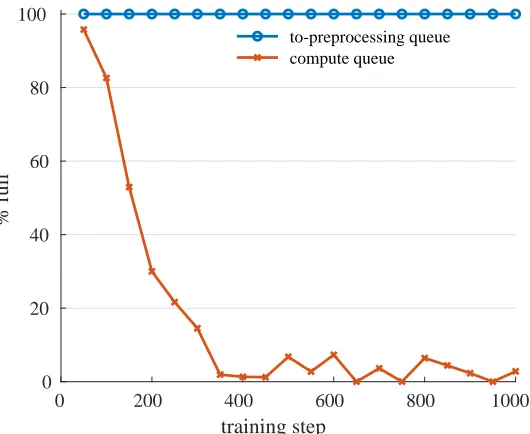
Figure 3.1: For the default single pipeline, the preprocessing queue is always full, while the compute queue empties quickly. Thus the preprocessing task is the bottleneck.
Thus we use Tensorboard5summaries on the various queue sizes in the pipeline to determine
where bottlenecks might be occurring. Since the operation that saves summaries in Tensorflow can
affect training performance, we save summaries every 20 steps and disable certain costly summary
operations, such as preprocessed image viewing. We run Alexnet for 1000 steps on the ImageNet
dataset, then analyze the relevant queues in Tensorboard.
Figure 3.1 shows the measured size of the preprocessing and compute queues during the training
process. As shown before in Figure 1.2, the preprocessing queue is the data that is about to be
preprocessed, and the compute queue is the preprocessed data being fed to the DNN. In this case,
the preprocessing queue fills up quickly enough that the summary data for this queue reports that it
is always full. On the other hand, the compute queue fills up during the startup phase, then empties
out in the first few hundred steps. In Tensorflow, the first step of the training process is typically
many times slower than the rest. This is primarily due to various initialization and optimization
5Tensorboard is a diagnostic tool designed to parse and display summary data produced during a Tensorflow training
routines that are being executed at runtime. The result is that the batch queue has time to fill while
the first step is executing, but cannot keep up after the first step. The bottleneck in this case is
therefore the preprocessing stage.
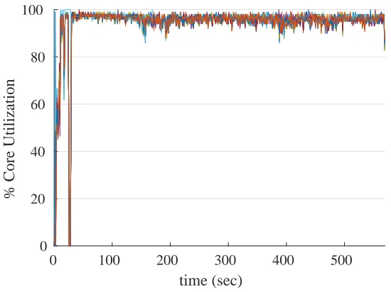
0 100 200 300 400 500
time (sec)
0 20 40 60 80 100
% Core Utilization
Figure 3.2: Default single pipeline core utilization for each of the 16 cores on a single Titan node when training Alexnet. The average core utilization over the entire graph is 94.3%. When the startup phase is excluded, the average is 96.0%.
It is important to show that the preprocessing uses the entire CPU. Figure 3.2 shows the
utiliza-tion level for each of the 16 cores in our default single pipeline test. Once Tensorflow has finished
initializing, we see the utilization reach peak levels and remain there. The average measured
uti-lization for this test was 96.0% after startup. From these series of tests, we conclude that a heavy
preprocessing load with a smaller DNN is capable of shifting the bottleneck from the model
train-ing to the preprocesstrain-ing. More computationally intense models (e.g., GoogleNet with Inception
modules) can also create similar issues on newer hardwares like NVIDIA V100 with TensorCore
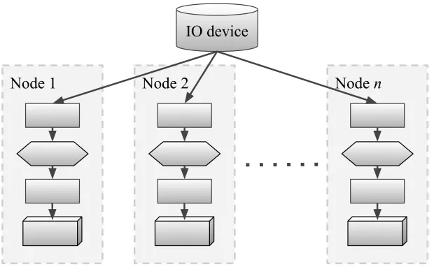
Node 1
Node 2
IO device
Node
n
Figure 3.3: Duplicated pipelines that can be used to concurrently train DNNs.
3.3.2 Multiple Nodes
The natural extension to the single pipeline in Figure 1.2 is to duplicate each pipeline for each DNN
in an ensemble. This duplicated pipeline is shown in Figure 3.3. In theory, each DNN could be an
arbitrary network, but our present tests use the same network for the sake of analyzing optimization
potential.
We first note two main concerns arising from the duplicated pipeline. First, each node reads its
own copy of the dataset, which is highly redundant and places unnecessary strain on the storage
systems6. High IO usage could in theory lead to scalability problems. Second, the preprocessing
operations are redundant since the same data is being modified. While this does not present
scala-bility problems, it does result in unnecessary CPU usage. As shown earlier in Figure 3.2, the CPU
usage could actually be quite high. This presents some opportunities for pipeline optimization.
In order to test potential scalability issues, we perform a test of the duplication pipeline on 1000
nodes of Titan and compare overall training time to that of nodes run individually. Table 3.1 shows
the results of executing 2000 steps of Alexnet on 1000 nodes of Titan in parallel, as well as the results
6Unless the file-system uses caches and each node is reading data from the same files in such a way that the cache
Table 3.1: Statistics comparing the total run time for 50 solo runs and a parallel run of 1000 nodes for 2000 Alexnet steps.
Avg Std Dev Min Max
Solo 1132.3 1.429 1129.7 1134.5
Parallel 1132.2 1.962 1125.0 1139.0
of executing 50 nodes individually. While the 1000 nodes exhibited slightly higher variance in its
runtimes, the overall runtime was not affected. This demonstrates that the storage systems in Titan
Chapter
4
Optimized Pipelines
Keeping in mind the issues with the duplicated pipeline discussed in the previous chapter, we
establish three objectives for designing pipelines to increase system efficiency:
1. Eliminate pipeline redundancies through data sharing.
2. Enable sharing by increasing pipeline flexibility.
3. Use increased flexibility to accelerate the pipeline.
Towards these goals, we focus on balancing the computational demand for preprocessing and model
training. Fortunately, ensemble training provides access to more CPU power for the same data,
thereby yielding an opportunity to accelerate the preprocessing stage.
4.1
Problem statement
Letnbe the total number of DNNs being trained. Since each DNN uses a single compute node,n
is also the number of nodes being used for the ensemble training. Letpbe the number of nodes
after the communication stage. Note that for simplicity of notation,Drefers to the dataset at any
stage of the pipeline, either before or after being preprocessed.
Given a particular DNN and hardware system, letrc be the GPU’s compute throughput, and
letrp be the CPU’s preprocessing throughput. Both can be measured in units ofimages/second. In
order to achieve maximum training speed, we needrp≥rc. However, this may not be the case, as we have already shown with Alexnet on Titan. A solution to this challenge is to share preprocessing
steps acrossnmachines for each data partition, which can raise the throughput of preprocessing
up ton rp≥rc.
Taking this approach, the number of machines,nneeded to satisfyn rp≥rc was relatively small
for our test cases. For example, our tests revealed thatn=2 is theoretically sufficient to saturate
Alexnet’s compute rate. If more advanced preprocessing techniques are used to enhance model
training, the computational requirements on the CPU will increase and may require largern to
satisfy the condition.
In practice,n rpis only an upper bound on the possible preprocessing rate. After the data has
been prepared, it must be shared over the cluster’s network to each training node. Therefore, the
peak preprocessing throughput for each node becomes a function ofn, say peak(n)≤n rp. Asn
increases, the upper limits of peak(n) depend on the communication pattern among nodes for
preprocessing and the network capabilities of the cluster. To address this issue, we need to consider
flexible pipeline designs in order to accelerate the progress of the pipeline. Later on, we will show
detailed empirical results in this regard.
In the remainder of this chapter, we introduce our method for improving pipeline flexibility, and
further explore different communication patterns as alternatives to the baseline of the duplicated
4.2
Horovod groups
Horovod[27]is a distributed deep-learning library for Tensorflow. Although distributed
Tensor-flow[3]provides implicit tensor sends and receives, it does not provide collective operations.1
Horovod fills the gap by supporting collective operations, including all-gather, broadcast, and
all-reduce. Thus, it allowstensorobjects to be sent through MPI collectives.
However, one limitation in Horovod is its master-worker communication structure. It is designed
to operate in “ticks”, each consisting in a series of operation requests to the master, followed by adone
message. Such a structure forces all communication to occur on a global scale, specifically, using
MPI_COMM_WORLD as the communicator for MPI messages. When designing custom pipelines,
we need the ability to use MPI collectives within a subset of ranks.
To solve this issue, we developedHorovod Groups[25]. This modification allows the user to
provide a list of groups that should be created upon initialization of the library. Whenever a collective
tensor is created, a group index must then be provided indicating which communicator to use for
the operation. At present, there are no known constraints on the memberships within these groups.
For example, two groups need not be mutually exclusive. A particular rank launches a background
MPI thread for each group to which it belongs. Communication can then occur asynchronously
using multi-threaded MPI.
1
2
3
1
2
3
1
2
3
1
2
3
Figure 4.1: Visualization of the MPI all-gather collective.
1A “collective” in MPI is an operation that sends a series of messages between usually more than 2 ranks, typically with
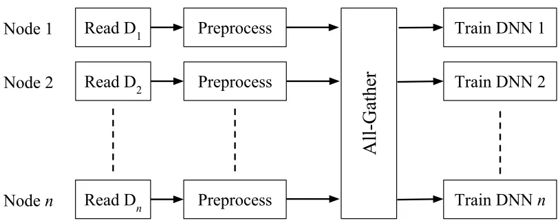
Read D
1Preprocess
Node 1
Train DNN 1
All-Gather
Read D
2Preprocess
Node 2
Train DNN 2
Train DNN
n
Read D
nPreprocess
Node
n
Figure 4.2: Illustration of the All-Shared (AS) pipeline. The datasetDis divided intonpartitions for each reader.
4.3
All-Shared
To share preprocessed data with all nodes, one possible approach is to make every node a
prepro-cessor (n=p), and share each node’s data with all other nodes. The MPI all-gather operation (see
Figure 4.1) is well suited to this purpose. We refer to this as theAll-Shared(AS) pipeline, as depicted
in Figure 4.2.
The first benefit of this design is its implementation simplicity. Horovod does not need to
be modified since we can use the built-in all-gather operation, and the code changes required
to implement it are minimal. These changes involve inserting an all-gather operation after the
preprocessing stage, but before the compute stage. Inserting additional queuing stages before and
after this operation may be recommended in order to avoid unwanted latency. A secondary benefit
is its high potential efficiency. Since every node contributes to the preprocessing stage through a
single collective operation, individual nodes may need to do very little work depending on the size
of the ensemble.
neural network models, it seems unnecessary to require that every node instantiate a data reader
and preprocessing stage, when a small number of nodes could provide enough preprocessed data
to training models. Our next two designs attempt to take advantage of this fact, thereby increasing
their flexibility.
4.4
Single-Broadcast
We now wish to allow the number of preprocessorsp to be adjustable. Suppose nodes 1, . . . ,pare
the preprocessor nodes, andp+1, . . . ,n are nodes that only contain the GPU’s compute stage.
Presumablyp<n, since ifp=nwe could use the All-Shared technique.
As a first step, we can perform an all-gather between the preprocessor nodes 1, . . . ,p. Now each
of these nodes has access to all the data, but the remainingn−p nodes have none. One method to resolve this is to elect nodepto broadcast its data out to nodesp+1, . . . ,n. This process is shown in
Figure 4.3, and we refer to this pipeline asSingle-Broadcast(SB).
The benefit of this pipeline is increased flexibility over AS. We can now control the value ofpto
adjust the pipeline as necessary to our particular application. The primary downside to this design
is potentially degraded performance, since rankpnow needs to perform two collective operations.
Additionally, Horovod Groups is needed for its custom MPI communicators.
4.5
Multi-Broadcast
Each nodeiin 1, . . . ,phas its own data itemDi. Instead of running an all-gather between
prepro-cessors, eachicould broadcast itsDi to all other nodes. In Multi-Broadcast, we avoid the initial
all-gather by performing asynchronous broadcasts from each preprocessor, as shown in Figure 4.4.
The benefit of this design is its evenly distributed approach. Each preprocessing node has
identical work without the extra demand placed on rankpby Single-Broadcast. However, it is limited
in the number of preprocessing nodes it can create efficiently, since each broadcast operation needs
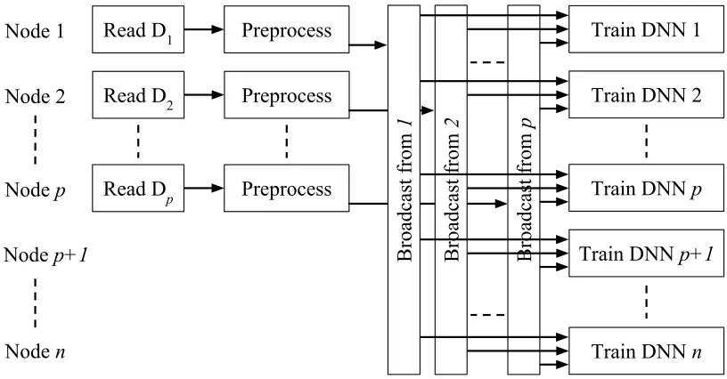
Read D
1Preprocess
Node 1
Train DNN 1
All-Gather
Read D
2Preprocess
Node 2
Train DNN 2
Train DNN
p+1
Node
n
Train DNN
p
Read D
pPreprocess
Node
p
Node
p+1
Broadcast from
p
Train DNN
n
Figure 4.3: Illustration of the Single-Broadcast (SB) pipeline. The datasetDis divided intop parti-tions for each reader instead ofn, since there are nowp readers feeding their own preprocessor.
Read D
1Preprocess
Node 1
Train DNN 1
Read D
2Preprocess
Node 2
Train DNN 2
Train DNN
p+1
Node
n
Train DNN
p
Read D
pPreprocess
Node
p
Node
p+1
Train DNN
n
Broadcast from
1
Broadcast from
2
Broadcast from
p
Figure 4.4: Illustration of the Multi-Broadcast (MB) pipeline. Similar to the Single-Broadcast design, the dataset is divided intoppartitions. EachDifor 1≤i≤pis broadcasted to all nodes with thei’th
Chapter
5
Metrics for Evaluation
In this chapter we introduce some of the metrics used to compare the baseline and our alternate
pipeline designs.
5.1
Peak Preprocessor Throughput
Previously we defined peak(n)as the function representing the maximum image throughput in
a pipeline for a given number of nodesn. The peak function is a good method to measure the
scalability of a pipeline, and provides the best mechanism for speed comparison to other pipelines.
While it is easy to think of peak(n)as a single function, it is actually defined by the throughput
at each node in the ensemble. However, it turns out that for a queuing system with finite size, the
long term average throughput for each node should be the same.1Thus only one function is needed
to define the entire pipeline’s peak throughput.
Note that peak(n)is only a measure ofpreprocessingimage throughput, and does not involve
any DNN training. In order to test the value of this function for a specific pipeline, we construct the
compute queue that stores batches ready to be trained, then we dequeue a batch. Repeating this
1The long term averages are identical simply due to the nature of the collective communication. All nodes in the
pipeline receive all data. If nodeagets ahead of nodebin its computation, the images thatbhas not processed must be within a queue after the collective communication. Since these queues have finite size, the difference in progress between
operation quickly enough causes the pipeline to reach peak image throughput.
The importance of measuring peak(n) is apparent when the compute throughputrc is also
considered. As mentioned before, we must have peak(n)≥rc in order to saturate GPU resources.
Towards this end, we additionally gather the value ofrc for each DNN in our tests. To obtainrc, we
calculate the average step duration for a specific DNN, while also pausing between steps to allow all
queuing systems to catch up. This ensures that the GPU will have data ready to be dequeued when
the next step is timed. By averaging the seconds per step, we then invert and multiply by the batch
size to obtain images per second, orrc.
5.2
CPU Usage
As a standard, it is important for the optimized version to run with at least the same training rate as
the baseline. However, it is not expected for the optimized pipeline to train DNNs faster than the
baseline under normal conditions. We previously established that it is possible for preprocessing to
form a bottleneck, but this is a more unusual case. If preprocessing is not a problem, our optimized
pipeline should not increase the training rate. In most of our tests, the GPU performance was the
limiting factor. Recall that this may change when Summit becomes available, since there are many
more GPUs on the new node architecture. To measure overall CPU load, we use thempstatcommand
to obtain CPU utilization statistics on each compute node in 4 second intervals. After training is
complete, we integrate CPU utilization statistics over time to obtain CPU usage for the job.
5.3
Core Usage Limits
Another useful metric is the runtime of the training process when a CPU core limit is imposed.
Some cluster systems allow nodes to be shared by users who have requested few CPU cores for
their job. The charge allocated to the user’s account for such a job is typically only charged for the
number of cores allocated. In such a case, there is a clear benefit to allocating less cores if the job
cores used, and then compare the overall runtime to the baseline under the same limits. Since Titan
does not support node sharing nor partial core allocation, we simulate a limited CPU environment
by controlling the number of threads allocated to each MPI rank2. Since each rank is allowed to use
an entire node, the number of threads corresponds to the number of CPU cores allowed. Table 5.1
shows the average core usage when simulating 3 cores allocated on a single Titan node and training
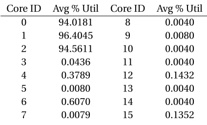
Alexnet on a basic pipeline.
Table 5.1: Average core usage when using simulated 3 core allocation on a Titan node.
Core ID Avg % Util Core ID Avg % Util
0 94.0181 8 0.0040
1 96.4045 9 0.0080
2 94.5611 10 0.0040
3 0.0436 11 0.0040
4 0.3789 12 0.1432
5 0.0080 13 0.0040
6 0.6070 14 0.0040
7 0.0079 15 0.1352
5.4
Energy Usage
A secondary benefit from decreased CPU usage is power savings. Most modern CPUs automatically
decrease clock frequency3in order to save power when no instructions are being fed. Therefore it
seems reasonable to expect some energy savings if CPU usage is reduced significantly. While it is
sometimes possible to obtain CPU or GPU power readings directly through software, Titan does not
provide this capability.
Instead, we collect energy consumption data through 2 metered cabinets. Each of these cabinets
includes 96 nodes, 8 of which are service nodes, leaving a total of 88 nodes for user jobs. The
major limitation of these cabinets is that they only record the consumption of theentirecabinet, so
distinguishing between the power usage of different devices within the cabinet is impossible. Thus
the results we report are the power consumption of all devices in the cabinet, not just the CPU.
In order to eliminate possible power variances due to jobs executing on different systems, we
reserved only one cabinet for all jobs. We submit each ensemble training job sequentially, with
approximately 2 minute breaks between the job’s end and the next launch. Additionally, we launch
each type of job twice to obtain some measure of redundancy and confidence in our results.
Executing jobs within these cabinets requires a special reservation request filed through a
web-form, along with some setup from the OLCF staff. After the reservation, the technicians send the
energy report containing the Kilo-Watt consumption at specific date-times. In order to accurately
measure the usage of each job launched during the reservation, our program prints a time-stamp at
the beginning and end of training. After receiving the data, we find all power entries that fall within
Chapter
6
Experiments and Results
This chapter will provide experimental results to show the benefits that can be gained from
alter-native pipelines. We first measure the throughput capabilities of each pipeline architecture over
varying numbers of ensemble nodes. Such a measurement provides a rough idea of the performance
of each design, allowing us to remove those that are slow. For the best pipeline, we then measure
the amount by which the CPU usage is reduced, which we refer to as CPU reduction. Additionally,
we test the speedups obtained when the number of usable CPU cores is reduced. As a final measure,
we provide data on the energy that a Titan cabinet consumes when training the baseline and our
best pipeline.
Table 6.1: Titan cluster specifications.
Processor 16-Core AMD
GPU K20X Kepler
Architecture Cray XK7
Interconnect Gemini
Number of cabinets 200
Table 6.2: Characteristics of the DNNs used in our tests. The layers and parameters data was obtained from[19, 18, 34, 29]. The compute rate, in units of images-per-second, is our measurement of the rate at which each DNN can consume preprocessed data when using the specified batch size.
DNN Batch Size # Layers Deep # Parameters Compute Rate (images/sec)
Alexnet 128 8 60M 306
Inception V1 32 22 6.8M 69
VGG-A 32 11 133M 31
6.1
Methodology
All experiments reported in this chapter were performed on the Titan cluster at Oak Ridge National
Laboratory using Tensorflow version 1.3.0. Titan’s specifications are provided in Table 6.1.
The input data for the pipeline was part of the ImageNet dataset, and included approximately
1.2 million images. Images sometimes have varying sizes, so the preprocessing stage resizes the
images to 224×224, which is the required dimensions for the first layer in our test networks. We choose this dataset because preprocessing is more expensive on larger images.
The Slim module[4]provides the preprocessing mechanisms needed to prepare images for
training. This module also provided Tensorflow implementations of the three DNNs used in our
tests, namelyAlexnet,Inception V1, andVGG-A. Some of the basic specifications of these DNNs
are provided in Table 6.2. Different versions of these networks are commonly used by the research
community for performance and accuracy benchmarks[5, 6, 8, 15, 16, 30].
The motivation for using these three networks is their varyingcompute rates. This is the rate at
which each DNN consumes preprocessed images. We measure this value experimentally in units of
images/secon Titan. Note that the compute rate is the key factor that influences the preprocessing
stage. A high rate will place extra demand on the CPU for image preprocessing, which will result
in high CPU utilization. Alexnet is well-suited for this purpose. On the other hand, Inception and
especially VGG require a smaller data rate, and so the CPU is used much less. In order to produce
meaningful results, we must demonstrate that our pipelines will produce savings over such a range
0 50 100 150
# nodes (n)
0 100 200 300 400 500 600 700 800 image/sec Alexnet Inception V1 VGG-A All-Shared SB-npre=5 SB-npre=20 MB-npre=5 MB-npre=20
(a) Full 16-core testing up to 150 nodes.
0 10 20 30 40 50
# nodes (n)
0 100 200 300 400 500 600 700 800 image/sec Alexnet Inception V1 VGG-A All-Shared SB-npre=5 SB-npre=20 MB-npre=5 MB-npre=20
(b) Partial 4-core test up to 50 nodes.
6.2
Peak Throughput
In order to effectively compare each pipeline to find the best, we first observe differences in peak
throughput of the preprocessing stage, or peak(n). Recall that this function is a measure of the
steady state image throughput for the preprocessing stage, and does not include any DNN training.
Figure 6.1a shows the value of peak(n) forn≤150 for increments of 5 nodes. Since the SB and MB pipelines each also needppreprocessors, technically we need to illustrate peak(n,p). For simplicity,
the figure shows peak(n, 5) and peak(n, 20). We observe that changing the number of preprocessors
between 5 and 20 does little to affect the throughput asnincreases. Furthermore, the SB and MB
pipelines are incapable of saturating Alexnet, since they drop below itsrc line. Despite their poor
performance, they still provide a viable mechanism to train larger networks, as both Inception and
VGG are well within their compute demands.
In order to clarify this data when core usage is restricted, Figure 6.1b shows peak(n) for up to 50
nodes. The performance for SB and MB is markedly decreased, while AS remains unchanged. This
confirms that AS is better in terms of peak throughput for both full-core and partial core training.
0 10 20 30 40 50
# nodes 0
0.5 1 1.5
2 2.5
3 3.5
CPU usage (normalized to AS)
SB MB
For SB and MB, these results point towards the broadcast operation as a performance problem.
Asnincreases whilepremains constant, the broadcast size also increases. This correlates to the
slow decrease in throughput seen in Figure 6.1.
As a final test for the broadcasting pipelines, we compare the CPU usage for AS, SB, and MB in
Figure 6.2. We vary the number of nodes in the ensemble between 10 and 50 and normalize the
resulting CPU usage to the AS pipeline. The SB pipeline uses marginally more CPU than AS, while
MB uses far more. This indicates that both of these pipelines are inferior to AS in both preprocessor
throughput and CPU usage. Thus, our next series of tests are only performed on AS.
6.3
CPU
Figure 6.3 shows the reduced CPU usage provided by the AS pipeline. We see that the usage is
reduced by up to 10.8X, 3.5X, and 2.4X for Alexnet, Inception, and VGG, respectively. We observe
that the reduction is inversely proportional to the compute rate of the DNN being trained (compute
rate data is provided above in Table 6.2). The compute rate is the primary indicator of how much
0 10 20 30 40 50
# nodes
1 3 5 7 9 11
CPU Reduction
Alexnet Inception V1 VGG-A
CPU time is needed to preprocess data for the GPU. Higher demanding networks like Alexnet will
cause the preprocessing stage to use much more CPU, while Inception and VGG will use less. Thus
we see smaller reductions for larger/slower networks.
Aside from measuring CPU usage reduction, we also test training time when CPU limits are
imposed. Figure 6.4 shows the speedup that AS provides when both AS and the baseline are subjected
to core restrictions. Recall that each Titan node has a 16 core CPU.
Alexnet sees a speedup of up to 10X for 1 core allocation on the AS pipeline. To understand this,
Table 6.3 provides information on how each pipeline slows down under core limitations. From this
table, we see that Alexnet’s speedup is due primarily to the dramatic slowdown that the baseline
incurs (9.6X) from this limitation, since it relies on additional CPU power to preprocess data. In
contrast, the AS pipeline only incurs a 54% slowdown due to the severe core limitation. While the
AS pipeline’s large number of individual processor cores should in theory be able to handle the
1 2 4 8 12 16
# cores
13 5 7 9 11
Speedup
Alexnet Inception V1 VGG-A
Table 6.3: Slowdowns under a 1-core limitation, measured relative to the 16-core performance of the same DNN and pipeline.
Pipeline DNN 1-core slowdown
Alexnet 9.61X
Baseline Inception 3.49X
VGG 1.83X
Alexnet 1.54X
All-Shared Inception 1.06X
VGG 1.02X
necessary preprocessing, having only 1 core limits other systems as well from executing efficiently,
thus causing the slowdown. However, the AS pipeline is able to train Inception and VGG on 1 core
incurring only a 6% and 2% slowdown, respectively. Since less preprocessing is needed for these
networks, less competition for CPU resources is present, allowing near-full-speed training. As with
the CPU-reduction results, the potential speedups under core limitations is inversely proportional
to the size of the DNN being trained. To reiterate, this is simply because larger networks need less
CPU for preprocessing since they train slowly.
6.4
Energy Consumption
Figure 6.5 shows the power usage of the 12 jobs launched during the 6 hour reservation of the
metered cabinet on Titan. In order to accurately distinguish between each job, the ensemble program
automatically notes the beginning and end time of the execution. We can then use these times, as
shown in Table 6.4, to crop the data to each task run.
One important note for this data is the minimum and maximum energy recorded. We can
observe in Figure 6.5 that there is a high minimum energy usage for the cabinet around 18-20KW. We
used a different reservation left in an idle state (no jobs being run) to determine that the minimum
energy usage is almost precisely 19KW, with very little deviation. We also observed that the maximum
energy for the cabinet was exactly 32.767KW. This data is reported in Table 6.5. This indicates that the
0 1 2 3 4 5
time (hours)
0 5 10 15 20 25 30 35
KW
Cabinet KW Usage
Figure 6.5: Total power draw over entire cabinet reservation period. The 12 jobs run during this time are described in Table 6.4.
Table 6.4: Jobs launched during an 8AM - 2PM reservation on one power metered cabinet on Titan. Times are formatted ashh:mm:ss.
Start Time End Time Duration Pipeline Version DNN
08:05:37 08:18:06 00:12:29 All-Shared Alexnet
08:21:35 08:40:24 00:18:48 Baseline Alexnet
08:44:35 08:59:58 00:15:22 All-Shared Inception
09:03:35 09:19:31 00:15:56 Baseline Inception
09:23:38 09:36:05 00:12:26 All-Shared Alexnet
09:39:41 09:58:22 00:18:41 Baseline Alexnet
10:04:35 10:19:59 00:15:23 All-Shared Inception
10:23:43 10:39:39 00:15:55 Baseline Inception
10:44:42 11:18:36 00:33:54 All-Shared VGG
11:22:40 11:57:12 00:34:32 Baseline VGG
12:00:38 12:34:32 00:33:53 All-Shared VGG