Scholarship@Western
Scholarship@Western
Electronic Thesis and Dissertation Repository
4-17-2012 12:00 AM
Experimental and Numerical Study of Flow Structures Associated
Experimental and Numerical Study of Flow Structures Associated
with Low Aspect Ratio Elliptical Cavities
with Low Aspect Ratio Elliptical Cavities
Taravat Khadivi
The University of Western Ontario
Supervisor Dr. Eric Savory
The University of Western Ontario
Graduate Program in Mechanical and Materials Engineering
A thesis submitted in partial fulfillment of the requirements for the degree in Doctor of Philosophy
© Taravat Khadivi 2012
Follow this and additional works at: https://ir.lib.uwo.ca/etd
Part of the Aerodynamics and Fluid Mechanics Commons
Recommended Citation Recommended Citation
Khadivi, Taravat, "Experimental and Numerical Study of Flow Structures Associated with Low Aspect Ratio Elliptical Cavities" (2012). Electronic Thesis and Dissertation Repository. 462.
https://ir.lib.uwo.ca/etd/462
This Dissertation/Thesis is brought to you for free and open access by Scholarship@Western. It has been accepted for inclusion in Electronic Thesis and Dissertation Repository by an authorized administrator of
(Spine title: FLOW STRUCTURES ASSOCIATED WITH ELLIPTICAL CAVITIES)
(Thesis format: Monograph)
by
Taravat Khadivi
Graduate Program in Mechanical and Materials Engineering
A thesis submitted in partial fulfillment of the requirements for the degree of
Doctor of Philosophy
The School of Graduate and Postdoctoral Studies The University of Western Ontario
London, Ontario, Canada
ii
THE UNIVERSITY OF WESTERN ONTARIO School of Graduate and Postdoctoral Studies
CERTIFICATE OF EXAMINATION
Supervisor
______________________________ Dr. Eric Savory
Supervisory Committee
______________________________ Dr. Gregory Kopp
______________________________ Dr. Anthony Straatman
Examiners
______________________________ Dr. Girma Bitsuamlak
______________________________ Dr. Roger E. Khayat
______________________________ Dr. Gary Rankin
______________________________ Dr. Jun Yang
The thesis by
Taravat Khadivi
entitled:
Experimental and Numerical Study of Flow Structures
Associated with Low Aspect Ratio Elliptical Cavities
is accepted in partial fulfillment of the requirements for the degree of
Doctor of Philosophy
iii
Abstract
The flow regimes associated with a 2:1 aspect ratio, elliptical planform cavity in a turbulent flat plate boundary layer have been systematically examined for various depth/width ratios (0.1 to 1.0) and yaw angles (0° to 90°), using a combination of wind tunnel experiments (involving Particle Image Velocimetry and helium bubble visualization) and Computational Fluid Dynamics (CFD) simulations (employing three- dimensional steady calculations with the Reynolds Stress model turbulence closure). Satisfactory agreement has been found between the results using the two methods, indicating that the steady numerical simulations can be a cost-effective tool to predict the mean flow features.
The flow has been found to be highly dependent on yaw angle and cavity depth. For each of the three broad flow categories specified according to yaw angle, which include the symmetric flow regime (yaw angle = 0°), the straight vortex regime (yaw angle = 90°) and the asymmetric flow regime (15° ≤ yaw angle ≤ 60°) different regimes are found to
exist, depending on cavity depth. For each combination of yaw angle and depth, the flow has been analyzed through investigation of shear layer parameters, the three-dimensional vortex structure, pressure distribution and drag, wake flow, and vortex oscillations.
While the elliptical cavity flows have been found to have some similarities with those of nominally two-dimensional and rectangular cavities, the three-dimensional effects due to the low aspect ratio and curvature of the walls give rise to features exclusive to low aspect ratio elliptical cavities, including formation of cellular structures at intermediate depths and unique vortex structures within and downstream of the cavity.
iv
Keywords
v
Dedication
This thesis is dedicated, in loving memory, to my father Iraj Khadivi, who passed away
on July 28, 2011, while I was preparing this thesis. I know how important it was for him
to see me graduate, but he never got the chance. He was my hero and role model. His
beautiful heart was warm, nonjudgmental, and always open. I miss him every day of my
vi
Acknowledgments
It is my pleasure to thank the many people who made this thesis possible. My gratitude goes first and foremost to my advisor, Professor Eric Savory for his continued guidance, instruction, and encouragement. Also, I would like to thank him for his support and understanding during the difficult time I have been going through.
I am also grateful to Professor Gregory Kopp and Professor Horia Hangan for providing essential parts of the experimental equipment and facilities I have used in my research.
I want to acknowledge Mr. Christopher Vandelaar from University Machine Shop, whose professional services have been essential in preparation of my experimental setup. My sincere thanks go to Mr. Gerry Dafoe who was always willing to help and make equipment available at the Boundary Layer Wind Tunnel Laboratory.
I would like to thank my fellow graduate students, Mr. Adam Kirchhefer and Ms. Maryam Refan for helping me with the experimental setup and equipment, and also the members the Advanced Fluid Mechanics research group for their constructive comments.
My special appreciation goes to my loving, supportive, and patient husband, Dr. Arash Naghib-Lahouti, who has unconditionally supported me during my studies.
And finally, I would like to express my thanks to my late father Iraj, and my mother
vii
Table of Contents
CERTIFICATE OF EXAMINATION ... ii
Abstract ... iii
Dedication ... v
Acknowledgments... vi
Table of Contents... vii
List of Tables ... x
List of Figures ... xi
List of Appendices ... xx
Nomenclature... xxi
1 Introduction... 1
1.1 Gaps in Research on Elliptical Cavities... 2
1.2 Hypotheses... 3
1.3 Objectives of the Research... 5
1.4 Approach of the Current Investigation ... 6
1.5 Organization of the Thesis ... 7
1.6 Summary... 9
2 Literature Review... 10
2.1 Introduction... 10
2.2 A Brief Review of the Fundamental Concepts of Vorticity ... 11
2.3 Cavity Flow Classifications ... 17
2.4 Effect of Upstream Conditions on Cavity Flow ... 24
2.4.1 Cavity Flows ... 25
2.4.2 Backward Facing Step Flows... 29
2.5 Cavity Flow Oscillations... 33
2.6 Yawed Cavities ... 37
2.7 Different Cavity Planforms... 38
2.8 Drag of Cavities ... 40
2.9 Numerical Simulations of Cavity Flows... 45
viii
3 Numerical Simulation ... 56
3.1 Introduction... 56
3.2 Governing Equations ... 56
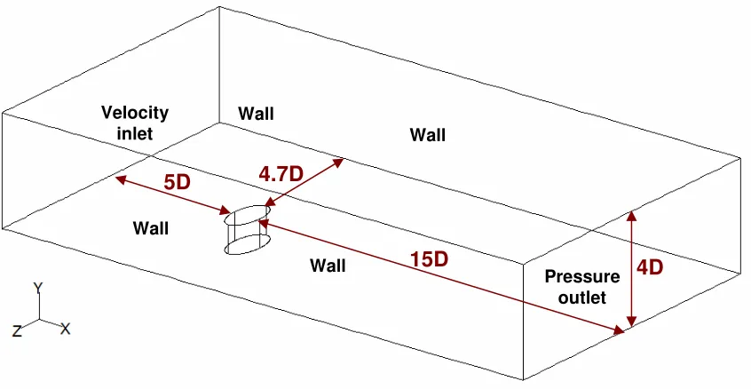
3.3 Computational Domain... 65
3.4 Computational Grid ... 66
3.5 Boundary Conditions ... 68
3.6 Solution Parameters ... 71
3.7 Validation of the Results of Numerical Simulations ... 72
3.8 Summary... 74
4 Experimental Methodology ... 76
4.1 Introduction... 76
4.2 Wind Tunnel ... 76
4.3 Model Specifications ... 77
4.4 Boundary Layer ... 87
4.5 Pressure Measurement Equipment... 90
4.6 PIV System ... 91
4.7 Flow Visualization ... 96
4.8 PIV Measurement Planes and Convergence Test ... 98
4.9 Experimental Uncertainty ... 100
4.9.1 Pressure Transducers ... 100
4.9.2 PIV System ... 101
4.10 Reference Velocity... 105
4.11 Detecting Vortex Core Position ... 110
4.12 Proper Orthogonal Decomposition ... 112
4.13 Summary... 113
5 Results and Discussion ... 115
5.1 Introduction... 115
5.2 Comparative Evaluation of the Experimental and Numerical Results ... 117
5.2.1 Comparison of PIV Experiments and Numerical Simulations ... 118
ix
5.3.1 Behaviour of the Shear Layer ... 130
5.3.2 Flow Structure... 133
5.3.3 Drag Characteristics... 144
5.3.4 Flow Downstream of the Cavity... 145
5.3.5 Flow Dynamics ... 151
5.3.6 Summary of Findings for Symmetric Flow Regimes ... 160
5.4 Nominally Two-Dimensional Flow Regime... 163
5.4.1 Behaviour of the Shear Layer ... 163
5.4.2 Flow Structure... 166
5.4.3 Drag Characteristics... 175
5.4.4 Flow Downstream of the Cavity... 176
5.4.5 Flow Dynamics ... 181
5.4.6 Summary of Findings for the Nominally Two-Dimensional Flow Regime 187 5.5 Asymmetric Flow Regimes... 190
5.5.1 Behaviour of the Shear Layer ... 191
5.5.2 Flow Structure... 193
5.5.3 Drag Characteristics... 208
5.5.4 Flow Downstream of the Cavity... 210
5.5.5 Flow Dynamics ... 213
5.5.6 Summary of Findings for the Asymmetric Flow Regimes ... 219
5.6 Summary... 221
6 Conclusions and Recommendations ... 224
6.1 Summary of the Findings... 224
6.2 Conclusions... 230
6.3 Recommendations for Future Work... 233
REFERENCES ... 236
Appendix A: Cavity Model Drawings ... 245
x
List of Tables
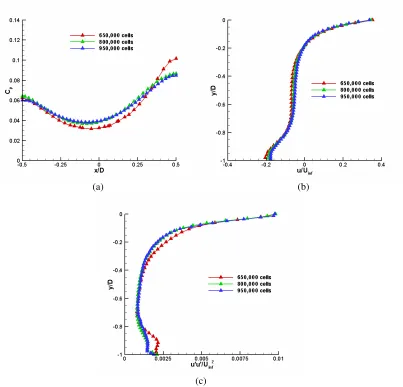
Table 3-1 Variations of selected parameters with the number of cells... 67
Table 3-2 Quantitative comparison of Cp values obtained by numerical simulations and experimental data ... 73
Table 4-1 Boundary layer parameters... 89
Table 4-2 The locations of vertical planes for different yaw angles... 98
Table 4-3 The locations of horizontal planes for different cavity depths ... 99
Table 4-4 Average variations of u and urms due to increasing the number of samples .. 100
Table 4-5 Total uncertainty of flow variables... 104
Table 4-6 u/Uinf for two yaw angles at two different locations (h/D = 1.0)... 109
Table 4-7 List of numerical simulation and experimental measurement cases ... 114
Table 4-8 Comparison of the parameters of present and Hering’s experiments [58]... 114
Table 5-1 Average distance between vortex cores (CFD & PIV results) ... 124
xi
List of Figures
Figure 2-1 General cavity variables shown for a rectangular cavity ... 11
Figure 2-2 Closed (a) and open (b) cavity flow regimes at subsonic speeds (adapted from ref. [14]) ... 18
Figure 2-3 Closed (a) and open (b) cavity flow regimes at supersonic speeds (adapted from ref. [14]) ... 19
Figure 2-4 Cavity base centreline pressure profiles (adapted from ref. [15])... 20
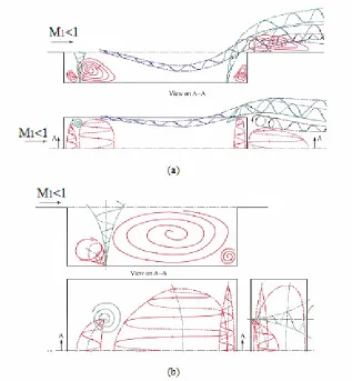
Figure 2-5 Main three-dimensional flow structures for rectangular closed (a) and open (b) cavities (adapted from ref. [14]) ... 21
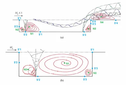
Figure 2-6 Topology of flow for closed (a) and open (b) rectangular cavities... 24
Figure 2-7 Mean flow field (adapted from ref. [24]) ... 28
Figure 2-8 Typical feedback resonance mechanism [53] ... 35
Figure 2-9 Schematic model of aerodynamic phenomena resulting in vorticity shedding [49]... 38
Figure 2-10 Resulting flow regimes of yawed elliptical cavities [6]... 40
Figure 2-11 Variation of normalized drag coefficient with h/D for rectangular cavities at 0° yaw angle (The line is added to visualize the general trend.) ... 43
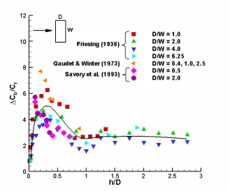
Figure 2-12 Variation of normalized drag coefficient with h/D for elliptical cavities at 0° yaw angle (The lines are added to visualize the general trend for elliptical (solid line) and circular (dashed line) planform shape.) ... 44
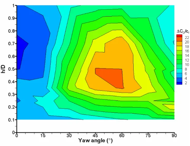
Figure 2-13 Effect of yaw angle and depth on the normalized drag coefficient of an elliptical cavity (W/D = 2) [58] ... 44
Figure 3-1 Typical velocity distribution in turbulent flow near a wall... 61
Figure 3-2 The turbulent boundary layer (adapted from ref. [75]) ... 62
Figure 3-3 Near-wall treatments (adapted from ref. [75]) ... 63
Figure 3-4 Geometry and boundary types ... 66
Figure 3-5 Computational grid in the cavity and the surroundings ... 67
Figure 3-6 Comparison of Cp (a), u/Uinf (b), and 2 inf /U u u′ ′ (c) for three different numbers of cells ... 68
xii
Figure 3-8 Dimensionless u'u' (a), v'v' (b), and u'v' (c) Reynolds stress profiles at the inlet
... 70
Figure 3-9 Turbulence kinetic energy (k) (a) and Turbulence dissipation rate (ε) (b) at the inlet ... 71
Figure 3-10 Comparison of Cp profiles on the centreline of the cavity base for three different h/D ratios at yaw angles of 0° (a) and 90° (b)... 73
Figure 3-11 Cp contours on cavity walls and around the cavity for h/D =1.0 at 0° yaw angle based on numerical simulation (a) and experimental results [58] (b) ... 74
Figure 4-1 Schematic representation of the wind tunnel [92]... 77
Figure 4-2 Schematic representation of the model ... 77
Figure 4-3 Cavity model and ground plate ... 78
Figure 4-4 Leading edge shape and surface roughness ... 79
Figure 4-5 Support leg ... 81
Figure 4-6 Trailing edge flap ... 82
Figure 4-7 Plate surface pressure coefficient upstream of the cavity in streamwise (a) and spanwise directions (b) for different combinations of yaw angle and the flap angle (α) ... 82
Figure 4-8 Velocity Profiles 1cm upstream of the cavity lip... 84
Figure 4-9 Two and three-dimensional obstacles ... 84
Figure 4-10 Velocity profiles comparison ... 86
Figure 4-11 Velocity profiles downstream a two-dimensional obstacle, solid line shows experimental data and dashed line shows the power law profile [103] ... 86
Figure 4-12 Comparison of the measured turbulent boundary layer data to the law of the wall... 88
Figure 4-13 Comparison of dimensionless u profiles (a) and u′v′ profiles (b) at seven upstream spanwise locations... 89
Figure 4-14 Example calibration curves for pressure transducers... 90
Figure 4-15 Images of the experimental setup, showing the main components: (1) model, (2) camera, (3) laser, (4) spherical lens, (5) laser beam reflector and cylindrical lens, (6) synchronizer, (7) imager recording computer ... 93
xiii
Figure 4-17 Dry ice placed at the upstream of the cavity (a) and inside the cavity (b).... 97 Figure 4-18 Helium bubble generator... 98
Figure 4-19 Effect of the number of samples on distributions of u (a) and urms (b) on a
horizontal line located at z/D = 0 and y/D = -0.6, for the cavity with h/D = 1.0 at yaw angle = 90º... 100 Figure 4-20 Image distortion for yaw angle = 90º (a) and yaw angle = 0º (b) ... 105 Figure 4-21 Velocity profile comparison for two different yaw angles at two different locations ... 107 Figure 4-22 The location of shear layer centre (h/D = 1.0) ... 108 Figure 4-23 Shear layer thickness... 109
Figure 4-24 Schematic figure of velocity profile at x/D = 0 (green line), contours of y u
∂ ∂
(red lines), shear layer (black dashed line), cavity walls (blue lines), and Uref
(black vector) ... 110 Figure 4-25 Different methods to find vortex core location inside the cavity (h/D = 1.0 & yaw = 90°)... 111 Figure 5-1 Different flow regimes of yawed elliptical cavity (adapted from ref. [6]). Symmetric, asymmetric and nominally two-dimensional regimes are highlighted in blue, red, and green, respectively. ... 117
Figure 5-2 Numerical and experimental results comparison of u and u'u'profiles for h/D = 1.0 at 90º yaw angle... 120
Figure 5-3 Numerical and experimental results comparison of u and u'u'profiles for h/D = 1.0 at 45º yaw angle... 121
xiv
Figure 5-7 Vortex core position (a) and pressure coefficient contours on cavity base, ground plane, and side walls for h/D = 0.5, yaw angle = 90º from reference [58] (b) and numerical simulations (c)... 129 Figure 5-8 Shear layer thickness at 0º yaw angle ... 131
Figure 5-9 The location of shear layer centre at 0º yaw angle... 132 Figure 5-10 Streamlines and Cp contours for cavity with h/D = 1.0 at 0° yaw angle at z/D
= 0 (a) and z/D = 0.7 (b) ... 134 Figure 5-11 Instantaneous flow visualization image obtained using the Helium bubble technique, for the cavity with h/D = 1.0 at yaw angle = 0º... 135 Figure 5-12 Vortex core positions and Cp contours at yaw angle = 0º for h/D = 0.7, 0.5,
and 0.35... 137 Figure 5-13 Sectional streamlines and Cp contours for cavity with h/D = 0.5 at 0° yaw
angle at z/D = 0 (a) and z/D = 0.7 (b) ... 138 Figure 5-14 Cp contours for a rectangular cavity (W/D = 3.18 & h/D = 0.5) at 0° yaw
angle (adapted from ref. [49])... 139 Figure 5-15 Cp contours at yaw angle = 0º for h/D = 0.5, Hering [58] (a), Savory and Toy
(adapted from ref. [5]) (b)... 140 Figure 5-16 Vortex core positions and Cp contours at yaw angle = 0º for h/D = 0.2 and
0.1... 142 Figure 5-17 Streamlines and Cp contours of cavity with h/D = 0.2 at 0° yaw angle (a) and
instantaneous streamlines of a nominally two-dimensional rectangular cavity with h/D = 0.13 [119] ... 142 Figure 5-18 Streamlines and and Cp contours for cavity with h/D = 0.1 at 0° yaw angle at
z/D = 0 (a) and z/D = 0.7 (b)... 143
Figure 5-19 Cp contours at yaw angle = 0º for h/D = 0.1 [58]... 144
xv
Figure 5-23 Quantitative comparison of velocity deficit at 0º yaw angle ... 150 Figure 5-24 Streamwise vorticity contours at x/D = 0.5 for h/D = 0.7 (a) and h/D =0.5 (b) at 0° yaw angle... 151 Figure 5-25 urms contours for h/D = 1.0 (a), 0.7 (b), and 0.5 (c) at 0° yaw angle at z/D = 0
... 153 Figure 5-26 Comparison of urms (a) and vrms (b) profiles on the vertical centreline ... 153
Figure 5-27 The first four POD modes of the fluctuating streamwise velocity component ... 154 Figure 5-28 The first four POD modes of the fluctuating vertical velocity component. 155 Figure 5-29 The first forty normalized eigenvalues for h/D = 1.0 (a) and 0.5 (b) at 0° yaw angle at z/D = 0 ... 156 Figure 5-30 vrms contours on vertical mid-plane (z/D = 0) by Oszalp (adapted from ref.
[29]) for a two-dimensional rectangular cavity (a), Haigermoser (adapted from ref. [54]) for a circular cavity (b), and the present study (c)... 156 Figure 5-31 Normalized time-varying coefficients for the cavities with h/D = 1.0 (a) and 0.5 (b)... 157 Figure 5-32 Phase averaged streamtraces in the vertical plane located at z/D = 0.35, for the cavity with h/D = 1.0. The phase interval between consecutive plots is 90°. ... 159 Figure 5-33 Phase averaged streamtraces in the vertical plane located at z/D = 0.35, for the cavity with h/D = 0.5. The phase interval between consecutive plots is 90°. ... 159 Figure 5-34 Schematic representation of the flow structure in an elliptical cavity in the symmetric-deep flow regime ... 161
xvi
Figure 5-39 Vortex core position (a) and pressure coefficient contours on cavity base, ground plane, and side walls for h/D = 1.0, yaw angle = 90º from reference [58] (b) and numerical simulations (c)... 167 Figure 5-40 Sectional streamlines and Cp contours for cavity with h/D = 1.0 at 90° yaw
angle at z/D = 0 (a) and z/D = 0.35 (b) ... 168 Figure 5-41 Example of mean velocity contours and streamlines in a nominally
two-dimensional rectangular cavity with h/D = 0.5 (adapted from ref. [122]).... 168 Figure 5-42 Instantaneous flow visualization images obtained using the Helium bubble technique, for the cavity with h/D = 1.0 at yaw angle = 90º... 169 Figure 5-43 Streamlines for cavity with h/D = 0.5 at 90° yaw angle at z/D = 0 (a) and z/D = 0.35 (b)... 170 Figure 5-44 streamlines of a nominally two-dimensional rectangular cavity (h/D = 0.25) (adapted from ref. [24])... 171 Figure 5-45 Cp contours for a rectangular cavity (W/D = 2 & h/D = 0.5) at 0° yaw angle
(adapted from ref. [49])... 171 Figure 5-46 Vortex core position (a) and pressure coefficient contours on cavity base, ground plane, and side walls for h/D = 0.1, yaw angle = 90º from reference [58] (b) and numerical simulations (c)... 173 Figure 5-47 Streamlines for cavity with h/D = 0.1 at 90° yaw angle at z/D = 0 (a) and z/D = 0.35 (b)... 174 Figure 5-48 Two-dimensional RANS computation of the flow pattern for h/D = 0.1 [123]
... 175 Figure 5-49 Comparison of Cp profiles on the centreline of the cavity base at yaw angle =
90° from numerical simulations (a) and reference [58] (b) ... 175
xvii
Figure 5-54 Streamwise vorticity contours at x/D = 1.0 for h/D = 0.7 (a) and h/D =0.5 (b) at 90° yaw angle... 180 Figure 5-55 Streamwise vorticity contours at y/D = 0.08 for h/D = 0.7 at 90° yaw angle
... 181
Figure 5-56 urms contours for h/D = 1.0 (a), 0.7 (b), and 0.5 (c) at 90° yaw angle at z/D =
0... 182 Figure 5-57 Comparison of urms (a) and vrms (b) profiles on the vertical centreline ... 182
Figure 5-58 The first four POD modes of the fluctuating streamwise velocity component ... 184 Figure 5-59 The first four POD modes of the fluctuating vertical velocity component. 184 Figure 5-60 The first forty normalized eigenvalues for h/D = 1.0 (a) and 0.5 (b) at 90° yaw angle at z/D = 0 ... 185 Figure 5-61 Normalized time-varying coefficients for the cavities with h/D = 1.0 (a) and 0.5 (b)... 185 Figure 5-62 Phase averaged streamtraces in the vertical plane located at z/D = 0, for the cavity with h/D = 1.0. The phase interval between consecutive plots is 90° 186 Figure 5-63 Phase averaged streamtraces in the vertical plane located at z/D = 0, for the cavity with h/D = 0.5. The phase interval between consecutive plots is 90° 186 Figure 5-64 Schematic representation of the flow structure in an elliptical cavity in the nominally two dimensional-deep flow regime ... 188 Figure 5-65 Schematic representation of the flow structure in an elliptical cavity in the nominally two dimensional-intermediate depth flow regime ... 188 Figure 5-66 The location of shear layer centre at 30º yaw angle... 192 Figure 5-67 Shear layer thickness for h/D = 0.5 at different yaw angles ... 193
Figure 5-68 Vortex core positions and Cp contours at yaw angle = 15º for h/D = 1.0, 0.5
and 0.1... 195 Figure 5-69 Vortex core positions and Cp contours at yaw angle = 30º for h/D = 1.0, 0.5
and 0.1... 196 Figure 5-70 Streamlines and Cp contours for cavity with h/D = 1.0 at 30° yaw angle at
xviii
Figure 5-71 Cp contours at yaw angle = 30º for h/D = 0.5 for a 2:1 elliptical cavity [58]
and a 2:1 rectangular cavity (adapted from ref. [49]) ... 198 Figure 5-72 Vortex core positions and Cp contours at yaw angle = 45º for h/D = 1.0, 0.5
and 0.1... 201
Figure 5-73 Vortex core positions and Cp contours at yaw angle = 30º for h/D = 1.0, 0.5
and 0.1... 202 Figure 5-74 Instantaneous flow visualization image obtained using the Helium bubble technique, for the cavity with h/D = 1.0 at yaw angle = 45º... 203 Figure 5-75 Cp contours at yaw angle = 45º for h/D = 0.5, Hering [58] (a), Savory and
Toy (adapted from [5]) (b)... 204 Figure 5-76 Cp contours at yaw angle = 60º for h/D = 0.5 for a 2:1 rectangular cavity
(adapted from ref. [49])... 205 Figure 5-77 Cp distribution at two vertical planes inside the cavity... 206
Figure 5-78 Cp distribution contours on cavity base (a) and Cp distribution contours and
velocity vectors in three horizontal planes inside the cavity (b)-(d)... 207 Figure 5-79 Schematic representation of the flow structure in an elliptical cavity in the strongly asymmetric flow regime ... 208 Figure 5-80 Comparison of drag coefficient for cavity with h/D = 0.5 at various yaw angles (The lines are added to visualize the general trend for each planform shape.) ... 209 Figure 5-81 Velocity deficit contours based on numerical simulations (left) and experimental measurements [58] (right) at 45º yaw angel ... 211 Figure 5-82 Streamwise vorticity contours at x/D = 0.7 for h/D = 0.7 at 45° yaw angle211 Figure 5-83 Velocity deficit contours based on PIV measurements in a horizontal plane at
45º yaw angle ... 212 Figure 5-84 Quantitative comparison of velocity deficit at 45º yaw angle ... 213 Figure 5-85 Comparison of urms (a) and vrms (b) profiles on the vertical centreline ... 214
xix
Figure 5-88 The first forty normalized eigenvalues for h/D = 1.0 (a) and 0.5 (b) at 45° yaw angle at z/D = 0.26 ... 216 Figure 5-89 Normalized time-varying coefficients for the cavities with h/D = 1.0 (a) and 0.5 (b)... 217
Figure 5-90 Phase averaged streamtraces in the vertical plane located at z/D = 0.26, for the cavity with h/D = 1.0. The phase interval between consecutive plots is 90° ... 218 Figure 5-91 Phase averaged streamtraces in the vertical plane located at z/D = 0.26, for the cavity with h/D = 0.5. The phase interval between consecutive plots is 90° ... 218 Figure 5-92 Comparison of urms values for three different yaw angles at 0.1D downstream
xx
List of Appendices
xxi
Nomenclature
A Dimensionless drag parameter (function of h/D)
a POD time varying coefficient
B Dimensionless drag parameter (function of M)
CD Drag coefficient
∆CD Incremental drag coefficient due to cavity presence
Cf Local skin friction coefficient
Cp Mean pressure coefficient, ( P -Pstatic)/Pdynamic
D Cavity minor axis
e Absolute uncertainty
h Cavity depth
H Boundary layer shape factor, δ*/θ
k Turbulent kinetic energy
l Turbulent length scale
M Mach number
N Number of samples
P Mean pressure
Pdynamic Freestream dynamic pressure
Pstatic Freestream static pressure
rms Root mean square, 2
u
ReD Reynolds number based on cavity minor axis, UinfD/ν
Sij Shear strain rate
St Stokes number
Uinf Freestream velocity
Uref Reference velocity
u Mean velocity
uλ Kolmogorov velocity scales
xxii '
'u
u Reynolds stress component in streamwise direction
W Cavity width
x Streamwise coordinate
y Vertical coordinate
z Spanwise coordinate, probability of estimating the mean value within ±e
α Trailing edge flap angle
Γ Circulation
δ Boundary layer thickness (based on u = 0.99Uinf)
δ* Boundary layer displacement thickness
δω Vorticity thickness
ε Rate of strain, Dissipation rate
θ Boundary layer momentum thickness
κr Real part of the wave number
Λ Integral length scale
λ POD eigenvalue, Kolmogorov length scales
µ Dynamic viscosity
µt Turbulence viscosity
ν Kinematic viscosity
ρ Density of air
σx Standard deviation
τ' Shear stress across cavity mouth
τf Characteristic time scale of the fluid flow
τfD Time scale of macroscopic fluid motion
τfΛ Time scale of integral-scale turbulent motions τfλ Time scale associated with Kolmogorov scale τP Response time of a seeding particle
τw Wall hear stress
ϕ POD Mode (eigen function)
ψ Stream function
Ωij Vorticity magnitude
1 Introduction
The flow over cavities (surface cut-outs) is relevant to the aerodynamics of aircraft and road vehicles and has been investigated since the early 1930s. The main focus of the research has been drag reduction by removing or modifying cavities and reducing the noise associated with them. Drag reduction is a major challenge in aerodynamic design but there is usually room for improvement. For a typical civil transport aircraft, parasitic drag, which originates from skin friction, surface imperfections, and pressure drag of the non-lifting components, is about 3% of the total drag [1]. Reduction of the parasitic drag can improve the vehicle’s fuel economy without affecting its aerodynamic performance. As an example of the significance of aerodynamic refinement through drag reduction, a 1% reduction in aerodynamic drag for an Airbus A340 airplane operating in the long range mode will result in savings of about 400,000 litres of fuel per year [2].
Surface irregularities are mostly caused by design or manufacturing constraints on aircraft or road vehicles. These include landing gear wells, weapons bays, flap recesses, rivet depressions and recessed windows for airplanes [3] and truck beds, sun roofs and door gaps for automobiles [4]. Most of these examples can be adequately approximated by models of simple geometry such as cavities of rectangular, circular or elliptical planforms. This highlights the importance of a thorough understanding of the flow associated with three-dimensional cavities of various planform shapes and depths.
The present study is focused on three-dimensional cavities with elliptical planforms, as one of the most general and complex forms of cavities. Compared to three-dimensional cavities with rectangular planforms, the flow associated with an elliptical cavity is more complicated due to the curved sidewalls. Furthermore, unlike a three-dimensional cavity with a circular planform, the flow associated with an elliptical cavity is affected by yaw angle, due to its elongated planform shape.
planform shape, and yaw angle, as well as flow related parameters, including Reynolds number (laminar or turbulent flow), approaching boundary layer parameters, and Mach number. These parameters have been shown to have significant effects on all aspects of the flow inside and around cavities, including flow structure and vortices, pressure
distribution and aerodynamic forces, and flow dynamics. It is therefore not adequate to generalize the findings related to cavities with a given set of geometric and flow parameters to other combinations of these parameters, which may require dedicated studies.
Although many researches have been performed on cavity flow over the past eighty years, most of them have been focused on nominally two-dimensional rectangular cavities subject to laminar flows. Only a few studies were focused on three-dimensional cavities, which were mostly confined to rectangular planforms, parallel to the flow.
The elliptical cavities have been studied by a few investigators. Friesing [3] studied the effect of elliptical cavity depth and aspect ratio on the resulting drag. Savory and Toy [5] have studied the effect of yaw angle and cavity depth for the elliptical cavities with aspect ratio of 2:1 and noticed an increase in drag for certain yaw angles. Hering and Savory [6] have studied the elliptical cavities with aspect ratio of 2:1 with different combinations of cavity depths and yaw angles. They have investigated the associated drag for each case, and presented a classification of different flow regimes for elliptical cavities. The limited number of studies on elliptical cavity flow has left many gaps in this research field. These gaps are discussed in detail in the next section.
1.1 Gaps in Research on Elliptical Cavities
The review presented in Chapter 2 indicates that the physics of the flow associated with elliptical cavities has not been completely determined, because of the limited number of previous studies in this area. Certain gaps exist in the knowledge on the flow associated with elliptical cavities, which can be summarized as follows:
• While the three-dimensional effects caused by the presence of sidewalls, such as
three-dimensional vortical structures, are relatively well-documented for cavities with straight walls (rectangular cavities), little is known about these effects in the case of cavities with curved walls.
• Elliptical cavities have been found to have highly asymmetric flows at certain yaw
angles, and drag forces larger than those of comparable rectangular cavities. This behaviour has been observed in a few previous studies, based on surface pressure distributions and wake velocity measurements; however, the flow structure at these conditions has not been investigated in detail, and therefore little knowledge of the mechanisms leading to this behaviour is available
• The effect of yaw angle on flow structure, pressure distribution, and drag of elliptical cavities is different for cavities with different depths (deep,
intermediate-depth, and shallow cavities). Specifically, the high drag associated with strongly asymmetric flows is observed only for deep and intermediate depth cavities. The
reason for this behaviour has not been explained.
• Previous studies on elliptical cavities include surface pressure measurements,
which can provide evidence of the flow structure near the cavity surfaces. No measurement of the flow inside an elliptical cavity, which would make it possible to establish a detailed and comprehensive three-dimensional representation of the flow structure inside the cavity, has been reported in the past. Also, the knowledge on dynamics of the flow inside elliptical cavities is limited to pointwise measurements using hotwire anemometry or surface pressure data, and no description of the dynamic behaviour of the principal flow structures (such as the shear layer and vortices) are available, in the case of elliptical cavities.
1.2 Hypotheses
Definition of the objectives, direction, and scope of the research is based on the following hypotheses, which will be evaluated throughout the thesis:
• Significant changes occur in the flow, when a nominally two-dimensional cavity
is bounded by sidewalls. These changes are more pronounced for cavities with low aspect ratios. It is expected that the curvature of the sidewalls leads to additional three-dimensional effects in the flow, such as curvature and displacement of recirculation regions and the associated vortices, and more complicated secondary flow structures, and gives rise to flow features unique to elliptical cavities, especially for low aspect ratios.
• Different flow regimes have been observed in both nominally two-dimensional and finite aspect ratio rectangular cavities, depending on cavity depth. Similarly,
the flow regime in elliptical cavities is also expected to be dependent on the cavity depth, but the flow structure in these regimes may not necessarily be similar to
those of the aforementioned cavities, due to the presence of curved walls.
• It is hypothesized that various asymmetric flow structures exist in elliptical
cavities, depending on the combination of yaw angle and cavity depth. These flow structures are expected to have unique features due to the elliptical planform shape. It is also conceivable that the high drag observed for elliptical cavities at certain yaw angles is related to asymmetric flow structures similar to that of the circular cavity with h/D = 0.5.
• Considering previous studies on nominally two-dimensional and rectangular
• Based on the relationship between position of the vortex core and the
low-pressure regions inside the cavity, which will be verified for elliptical cavities in the present study, a quantitative relationship is expected to exist between vortex strength and pressure levels on cavity surfaces.
• The flow in the wake of the elliptical cavity is expected to show traces of the flow phenomena caused by presence of the cavity. Depending on these phenomena, which may include the separation bubble formed immediately downstream of the cavity, side-edge vortices, and trailing vortices formed in certain asymmetric flow regimes, the wake may be dominated by velocity deficit or vorticity. Drag of the cavity is expected to be larger in the cases in which the wake is dominated by velocity deficit.
• The dynamic phenomena of the flow in an elliptical cavity, including feedback
resonance in the shear layer, shear layer oscillations, and vortex oscillations, are expected to be dependent on the combination of upstream boundary layer properties and state, geometric proportions of the cavity, and yaw angle. Therefore, it is conceivable for the flow in the cavity to show different levels of oscillation for different combinations of the above-mentioned parameters.
1.3 Objectives of the Research
In order to evaluate the above-mentioned hypotheses, the following objectives have been defined for the present research:
• To establish a comprehensive three-dimensional representation of the flow structure in the elliptical cavity volume, in order to complement previous studies in which the flow structure is determined based on surface pressure
measurements.
• To determine the effects of wall curvature on the flow structure in elliptical
• To analyze the effect of depth on the flow structure inside and around elliptical
cavities, in order to identify the flow regimes and features affected by depth and to determine similarities and differences with cavities with other planform shapes.
• To investigate the effect of yaw angle on the flow structure inside and around elliptical cavities with various depths, and to determine the flow structure and mechanisms associated with the increased drag forces associated with strongly asymmetric flows.
• To analyze the flow in the wake of the cavity, in order to investigate effect of the
cavity flow phenomena on the wake
• To study the dynamic behaviour of the vortex structures in the cavity.
• To identify the underlying mechanisms from which the above-mentioned effects originate.
1.4 Approach of the Current Investigation
Fulfillment of the above-mentioned objectives requires investigation of the flow inside and around elliptical cavities for multiple combinations of geometric parameters, such as cavity aspect ratio, relative depth, and yaw angle, and flow parameters, including Reynolds number, and the thickness and state of the upstream boundary layer.
An investigation involving combinations of all of the above-mentioned parameters is beyond the time and facility resources available for the present research. Therefore, the
scope of the present research has been defined by limiting these parameters to values that cover an adequate range of flow regimes, and make it possible to compare the results of the present study to previous ones involving elliptical and rectangular cavities.
cavities with rectangular planforms. The cavity with a circular planform (which is a special case of elliptical cavity with an aspect ratio of 1:1), has also been studied experimentally in the past, and interesting three-dimensional flow features have been reported in both cases. The elliptical planform with an aspect ratio of 2:1 has been chosen
to examine the flow mechanisms in comparison with those reported with the above-mentioned cases. Combinations of six ratios of cavity depth to minor axis length (h/D), including 0.1, 0.2, 0.35, 0.5, 0.7, and 1.0, and six yaw angles, including 0°, 15°, 30°, 45°, 60°, and 90° have been analyzed.
With regards to the flow parameters including Reynolds number, and the thickness and state of the upstream boundary layer, an attempt has been made to adjust them so that they match or are close to those of previous studies involving elliptical cavities. As will be shown in the coming chapters, this makes it possible to compare the observations and results of the present study with those of the previous work. Details of the flow related parameters will be described in Chapters 3 and 4.
Particle Image Velocimetry (PIV) and CFD simulations are the most adequate measurement and analysis techniques for achieving the first objective, since they can be used to acquire information not only on the boundaries of the cavity, but also inside the cavity volume. Therefore, these techniques have been selected as the principal tools for the present study.
1.5 Organization of the Thesis
The methodologies implemented in the present research, the results of the measurements and simulations, and their analysis, are presented in the following chapters of this thesis, according to the following organization:
• In Chapter 2, a comprehensive review of the literature related to the flow in
measurements of cavity flow. The findings of the reviewed research work have been summarized at the end of the chapter, to specify the framework within which the present research has been defined.
• Chapter 3 describes the details of the methodology of the numerical simulations
conducted in the present study. The chapter includes detailed description of the governing equations and their discretization, description of the turbulence treatment approach, the simulation domain and its boundary conditions, the grid and sensitivity of the results to it, and validation of the numerical methodology adopted in the present study through comparison with previously published experimental data.
• Chapter 4 describes the details of the methodology of the experiments conducted
in the present study. The chapter starts with a description of the experimental equipment, including the wind tunnel, the model, and the flow measurement and
visualization equipment. This is followed by a description of techniques used to adjust the flow upstream of the cavity and the boundary layer parameters. The chapter also includes an analysis of the experimental uncertainties, considerations for selection of reference velocity, and methods for detection of vortex cores.
• Chapter 5 presents the results of the simulations and the experiments, with the objectives of providing a detailed explanation of the flow structure for various combinations of cavity depth and yaw angle, comparing the findings with those of previous studies involving elliptical cavities and other similar flows, and identifying underlying trends and flow mechanisms. The chapter starts with a qualitative and quantitative comparison of the results of the present study with previous studies involving elliptical cavities, to combine the results for description of the flow behaviour. This is followed by presentation and analysis of the results, including flow structure, pressure distribution, and flow dynamics, in three major categories elliptical cavity flows: Symmetric flow regimes, asymmetric flow
summary, in which similarities and differences of the results of the present study with previous work are highlighted.
• Chapter 6 presents the conclusions of the present research. In this chapter, the
findings presented in Chapter 5 are summarized with the objectives of identifying and describing the underlying trends and fluid mechanics phenomena leading to the observed flow structures, and highlighting the flow features unique to elliptical cavities. Based on the findings and trends observed in the present study, suggestions for future research are made.
1.6 Summary
2 Literature Review
2.1 Introduction
In this chapter, a comprehensive review of literature is presented. Considering that the flow inside the cavity is dominated by vortices, the fundamental concepts of vorticity are discussed at the beginning of the review. This is followed by presentation of cavity flow classifications defined for nominally two-dimensional rectangular cavities.
Later, the effects of upstream flow condition, such as boundary layer characteristics and flow state (laminar or turbulent), on cavity flow are reviewed. The unsteady nature of cavity flows is discussed and flow dynamic mechanisms, including feedback resonance and conditions leading to it, are introduced. This is followed by a discussion on the principal factors affecting the cavity flow, such as yaw angle, depth and cavity planform
shape. Cavity drag is another topic which is reviewed in this chapter.
It should be mentioned that most of the review of the cavity flows is based on experimental studies undertaken in wind or water tunnels. Computational fluid dynamics studies of cavity flows are discussed separately, to determine the best and the most feasible approach to perform the numerical simulation part of the present research.
Finally the key findings are summarized succinctly which leads to highlighting the gaps in the previous studies, which have been mentioned in section 1.1. The research hypotheses and objectives, as well as investigation approach have been defined accordingly in sections 1.2 to 1.4.
In the following paragraphs, D refers to the stream-wise length of the cavity (chord), W is the span-wise width of the cavity and h is the depth of the cavity. Aspect ratio is the cavity width to length ratio (W/D). Figure 2-1 shows these variables for a yawed rectangular cavity.
Figure 2-1 General cavity variables shown for a rectangular cavity
2.2 A Brief Review of the Fundamental Concepts of Vorticity
Flow in the cavity is dominated by one or more vortices, generated as a result of the interaction of the shear layer separated from the upstream edge of the cavity, and the cavity boundaries. Throughout the thesis, the vorticity contained in the shear layer, the vortices, and their interaction with the boundaries will be discussed in several instances. These discussions often rely on the fundamental concepts related to vorticity, which might not be mentioned in the discussion. The objective of this section is to provide a brief review of these concepts, which will support the discussions in the following chapters of the thesis.
The review includes some fundamental definitions, followed by an overview of the concepts of generation of vorticity, the relationship between vorticity and rate-of-strain, and diffusion and decay of vorticity.
• Definitions
Conceptually, vorticity is defined as the local angular rate of rotation in a fluid. This conceptual definition leads to the mathematical definition of vorticity, as the curl of the velocity vector: ur r r × ∇ =
ω
(2-1)A number of fundamental definitions are usually used to describe vorticity fields. As indicated by its definition, vorticity is a three-dimensional vector in a three-dimensional flow field. The line that is tangent to the vorticity vector in the flow field is called a “vortex line”. It can be proved mathematically that vortex lines at a solid boundary are orthogonal to the streamlines [7].
Vortex lines can form closed loops (finite but endless paths) within the flow field, or extend to the boundary (solid, free-surface, or infinite), but cannot end within the flow field [8]. A “vortex tube” is a virtual closed surface formed by a series of vortex lines. It is usually assumed to have a circular cross section. The integral of the vorticity component normal to the cross section of a vortex tube, across the cross section is known
as circulation. Circulation, given by Γ=
∫
⋅ SdS nr r
ω
, is a measure of the strength of thevortex tube, and is constant along the tube in the absence of viscous effects, such as the “cross-diffusive” mechanism described later in this section, and turbulent decay of vorticity.
The equation governing transport and diffusion of vorticity in the flow field is known as the Helmholtz equation, or vorticity transport equation. This equation is written for an incompressible, homogeneous fluid as follows:
ω ν ω
ω ω
ωr r (r.r)r (r.r)r 2 r
∇ + ∇ = ∇ + ∂ ∂
= u u
t Dt D
(2-2)
The material derivative on the right hand side of the equation shows the rate of change of vorticity (or angular velocity) for a fluid particle or element as it moves in the flow field.
It accounts for the effect of unsteadiness in the flow (through the term t ∂ ∂ωr
), as well as
movement of the fluid element from one point to another (through the term (ur.∇r)ωr ).
The first term on the left hand side of the equation ((ωr.∇r)ur) is called the processing
term. This term accounts for local amplification of vorticity because of velocity gradients. The effect of velocity gradients can be stretching of vortex filaments, or local tilting or
turning of them. The second term on the left hand side of the equation (ν∇2ωr ) accounts for diffusion of vorticity in the flow field due to viscosity [7].
• Generationof vorticity
The Helmholtz equation does not contain any generation term to account for creation of vorticity. The source of vorticity generation in homogeneous fluids is the boundary, and is included in the solution of the vorticity equation through wall boundary conditions. The physical effect of a wall boundary on the flow is the wall shear stress
( 0 = ∂ ∂ = y w y u µ
τ ), where y is the wall-normal coordinate. The shear stress leads to a
tangential force, which in turn causes angular acceleration, torque, and rotation of the fluid near the wall.
In the simplified case of a two-dimensional flow, the vorticity vector assumes the following form: } 0 , , 0
{ ∂u ∂y−∂v ∂x =
ω
r (2-3)At the wall boundary, ∂v ∂x=0, because the wall-normal velocity is zero. Therefore, the
boundary conditions at the wall becomes:
} 0 , , 0 { } 0 , , 0 { 1
0 u y τw
Therefore, ω0.τw =0. This is an important conclusion regarding the relationship between
vorticity and wall shear stress. It implies that at the wall, vorticity is tangential to the surface, and at a 90o angle to the shear stress. The other implication is that wall shear stress is not responsible for generation of vorticity. In fact, vorticity and wall shear stress
are two representations of the wall-normal velocity gradient, related by µ[7] and [9]).
The time rate of change of circulation in the vicinity of the wall boundary can be considered as a measure of generation of vorticity. In a two dimensional flow field, circulation a thin closed circuit in the vicinity of the wall can be approximated by:
(
u U)
δ
xδ
Γ= − (2-5)in which U is the flow velocity outside the near wall region. Circulation per unit length of the solid boundary is therefore Γ=u−U, and the time rate of change of circulation is:
dt dU dt du dt d − = Γ (2-6)
Substituting the conservation of momentum equation ( u
x p x u u t u dt
du 1 + ∇2
∂ ∂ − = ∂ ∂ + ∂ ∂ = ν ρ )
in the above equation, leads to the following equation for generation of vorticity:
dt dU u x p dt d − ∇ + ∂ ∂ − =
Γ 1 ν 2
ρ (2-7)
Several conclusions regarding generation of vorticity can be made based on this equation. The formula indicates that vorticity generation results from acceleration or initiation of motion of a boundary in the tangential direction, and tangential pressure gradients along a boundary. In the case of a flat plate boundary layer in uniform flow, for example vorticity is generated at the leading edge of the plate (which in practice has a finite radius) at a rate
of 2 2
1U , and is then transferred downstream and diffused into the thickening boundary
According to the equation above, a change in the direction of wall acceleration or pressure gradient leads to generation of vorticity with opposite sense at the wall. Also,
viscosity plays no role in generation of vorticity, but it has a major role in redistribution of vorticity after generation. The formula also indicates that vorticity generation is
instantaneous, and once it is generated, it cannot be lost by diffusion to the wall boundaries ([7] and [10]).
• Vorticity and rate-of-strain
Rate-of-strain in a two-dimensional flow is given by:
x v y u ∂ ∂ + ∂ ∂ =
ε
(2-8)There are extreme cases of a flow in which vorticity can exist without rate of strain, or vice versa. For example, in a flow with pure rigid-body type rotation, uniform vorticity exists, without any rate-of-strain. However, in most cases, a combination of both exists in
the flow.
For example, in a shear flow with parallel streamlines, in which velocity is different on each streamline, a specific relationship exists between vorticity and rate-of-strain. The flow motion near the wall boundary is parallel to the wall. Therefore, the wall acts as a
source of both vorticity and rate-of-strain. At the wall, =0 ∂ ∂
x
v , and rate of strain is
equal to vorticity. This is the reason why there is vorticity but no large scale vortex structures in a laminar boundary layer.
The relationship between vorticity and rate-of-strain can be used to identify vortices in a region where both vorticity and rate-of-strain exists. This is the concept of the Q-criterion for identifying vortices, which subtracts rate-of-strain from vorticity, to identify the boundary of a vortex [11].
(
u u u)
(
S)
Q= ii − ij ji = Ω − 2 1 2 1 , , 2
In the above-mentioned formula, S and Ω are the symmetric and anti-symmetric
components of ∇u; i.e. ( ) 2
1
, ,j ji i
ij u u
S = + and ( )
2 1
, ,j ji i ij = u −u
Ω . Thus, Q represents
the local balance between shear strain rate and vorticity magnitude. It should be noted that unlike vorticity, rate-of-strain can be generated not only at the boundaries, but also inside the fluid. Examples and more detail can be found in Reference [7].
• Decay of vorticity
The Helmholtz equation (Equation 2-2) and the equation of vorticity generation (Equation 2-7) show that vorticity cannot be lost by diffusion to the solid boundaries. The decay and loss of vorticity in a flow field occurs by a mechanism called “cross-diffusive” annihilation [7] and [9]). The concept of this mechanism is based on the fact that vorticity
of opposite signs is generated at different regions (or time intervals) in the flow field. When the vorticity of opposite signs is transferred into the flow field, they interact and cancel each other. This leads to net loss of vorticity in the flow field.
Morton cites the global condition for circulation, which states that the gross circulation in an enveloping contour of a bounded region with outer boundary at rest must be zero, and concludes that at any given time, there exists an equal strength of vorticity of opposite signs within the domain, which may in time lead annihilation of vorticity when they diffuse and interact, depending on the flow structure. This principle can be verified for several types of flow, which are bounded completely or in part by solid boundaries [7].
• Diffusion of vorticity
Vorticity is a diffusive quantity and the mechanism by which it diffuses is viscous
diffusion. Diffusion of vorticity is quantified by the ν∇2ωr term in the Helmholtz equation. Unlike linear momentum, diffusion of vorticity does not occur at the molecular
byν∇2vr in the Navier-Stokes equations), which in turn is related to velocity gradients in
the flow field.
The cavity flow structure is dominated by vortices, and is strongly influenced by vorticity dynamics. Many of the cavity flow studies that will be reviewed in the following sections focus on global phenomena in the cavity, such as drag, pressure distribution, and acoustics. The present study, however, focuses on the flow structure in the cavity, including vortices and their dynamic behaviour. The principles described in the previous paragraphs provide a theoretical basis for the analysis and description of the behaviour of these vortices, which will be presented in Chapter 5.
2.3 Cavity Flow Classifications
In the case of depressions or cavities, simple geometries were initially investigated to examine the effects of cavity dimensional ratios on aerodynamic drag. Most of these studies were conducted on two-dimensional rectangular slots normal to the flow direction [4] and [12]. In later studies, fully three-dimensional cavities with different geometries and approaching flow conditions have been examined. These investigations have shown that the cavity flow regime varies with geometry (depth to length ratio, aspect ratio, and planform shape), yaw angle, Reynolds number (laminar or turbulent flow), approaching boundary layer parameters, and Mach number [13]-[58].
In 1961, the effects of depth to length ratio for two-dimensional rectangular cavities were studied and classic definitions of the different flow regimes were introduced [13]. Distinct flow patterns arise for certain conditions and, in general, cavity flows have been classified into two distinct categories, “open” and “closed” cavities with a transitional
The term “closed” cavity refers to the case where the shear layer separates at the leading cavity lip and impinges on the cavity base near the middle of the cavity, as seen in Figure
2-2-(a). The shear layer then separates from the cavity base and passes over the downstream wall of the cavity. A stagnation point exists near the cavity lip of the
downstream wall. In this case two regions of flow recirculation exist, one aft of the rearward-facing front wall, the other ahead of the forward-facing rear wall [14]. This flow regime occurs for shallow cavities where the cavity depth is much smaller than the cavity length (h/D<<1).
The “Open” cavity regime occurs for cavities in which h/D>0.1 in the case of a rectangular cavity planform. In this regime, the shear layer separates at the upstream cavity lip and bridges the cavity opening. The stagnation point occurs slightly closer to the cavity lip on the downstream cavity wall when compared to the closed flow [14]. A stable vortex forms inside the cavity volume for open type flows, as noted by Roshko [4]. Different configurations are possible for the stable vortex depending on the ratio h/D. This captive stable vortex is driven by the separated shear layer spanning the cavity [4].
Figure 2-2 Closed (a) and open (b) cavity flow regimes at subsonic speeds (adapted from ref. [14]) D
h
(a)
The flow regimes are strongly affected by Mach number. The same categorization is possible for supersonic speeds as well. In case of closed cavities expansion fans are
generated at the upstream and downstream edges. For the closed regime, two shock waves, known as the impingement and exit shock waves originate from the cavity base.
In the case of open cavities two shock waves exist close to the two edges (Figure 2-3). For supersonic speeds two transitional stages, known as transitional-open and transitional-closed, were identified [14].
Figure 2-3 Closed (a) and open (b) cavity flow regimes at supersonic speeds (adapted from ref. [14])
Plentovich et al. studied the centre line (x-y plane at z = 0 on the cavity base) pressure coefficient pattern for a rectangular cavity subjected to subsonic (0.2<M<0.95) fully turbulent flow with a very thin boundary layer, to determine the effect of the flow regime on the centre line pressure distribution. They realized that for open flow the pressure is approximately uniform for a considerable extent and then increases near the downstream wall. For closed flow a plateau occurs and downstream of the plateau the pressure decreases to form a minimum, followed by a rise in pressure to a maximum. For transitional flow, the pressure over the forward portion is similar to that of the open flow,
and over the rearward portion is concave down (Figure 2-4) [15]. (a)
(b)
The other important geometrical aspect of cavity flow is the width of the cavity. Early studies have shown that, even in cavities with large span-to-chord ratios which would
normally be considered to have two-dimensional flow near their centre lines, the flow is in fact three-dimensional and wave like structures (also known as cellular structures) can
be observed across the span of the cavity. The number of cellular structures was dependent on the aspect ratio and cavity depth. The study by Maull and East [16], which deals with rectangular cavities with varying aspect ratios of width to streamwise length (W/D) and depth to streamwise length (h/D) documents the cellular structures in detail for the open cavity flow regime beneath turbulent boundary layer. At a constant width to length ratio (W/D = 9), as the cavity depth was increased (h/D decreased from 2.5 to 0.5), cellular structures with a fewer number of cells were observed. Also, for a constant depth (h/D = 0.5), when the width to length ratio (W/D) was increased from 2 to 5.5, the number of cellular structures increased from 2 to 6. The case of W/D = 2 and h/D = 0.5, in which 2 cellular structures were observed, is of particular interest, as it resembles a part of the findings of the present study, which will be discussed in Chapter 5.
For rectangular cavities where W/D<1 the side walls and corners greatly affect the flow inside the cavity. The schematic diagrams of flow structures for small width open and
closed rectangular cavities at subsonic speeds (Figure 2-5) illustrate the possible three-dimensional nature of the main flow [14].
Figure 2-5 Main three-dimensional flow structures for rectangular closed (a) and open (b) cavities (adapted from ref. [14])
The flow patterns suggest the following main flow structures within the closed and open cavities:
• Closed cavity (Figure 2-5-(a))
effects. A very weak lateral vortex forms between the front wall and the forward separation line, making a counter rotating flow region. On the cavity base just aft of the
front wall and close to the side walls, there are two weak separation nodes, which are associated with a pair of counter rotating vertical vortices. There are two other separation
nodes on the cavity floor, close to the side walls and at the extremities of the separation line, which are indicated by a pair of counter rotating vertical vortices. While the shear layer cascades over the front wall, the flow is entrained over the side walls. Because of the recompression action of shear layer rising to pass over the rear wall, some of the entrained flow is ejected from the side walls.
When this schematic is compared to cavity base centreline pressure profiles (Figure 2-4), it can be observed that there is a low pressure area near the upstream wall of the cavity which is associated with the recirculation region at the upstream corner. Downstream of the recirculation region, the pressure rises again. This is then followed by a pressure drop, which can be attributed to the shear flow approaching the cavity floor. Then, another pressure rise is observed just before the downstream wall, due to a stagnation region formed when the entrained flow exits the cavity.
The results of previous studies on the flow inside and around rectangular cavities indicate that for the cases in which the length (streamwise dimension) of the rectangular planform is much larger than its width (spanwise dimension), streamwise vortices are formed along the edges of the cavity sidewalls [14]. The mechanism leading to formation of these vortices is the “cascading” of the shear layer over the upstream edge of the cavity, which leads to entrainment of the flow into the cavity over the sidewalls. When this entrained flow passes over the sharp, 90-degree edge of the cavity sidewall, “side edge vortices” are formed. Further downstream, these vortices are lifted clear of the downstream wall,
• Open cavity (Figure 2-5-(b))
There are tandem rotating vortices, in the central spanwise region. There is also a small, weak corner vortex, which has a sense of rotation opposite to that of the strong rear vortex. Also there are two separation nodes on the cavity floor just aft of the front wall, which indicate a pair of counter rotating vertical vortices.
For deep open cavities, one large captive vortex usually dominates the flow and the two recirculation areas associated with corner vortices are either small or negligible. Therefore, as shown in Figure 2-4, the pressure on the centreline is more or less uniform, for the most part, and then increases near the downstream wall of the cavity. However, for open-transitional flow regimes, the upstream recirculation zone has a non-negligible size. In these cases, the pressure distribution shows a lower pressure near the upstream wall when compared to the open cavity flow type.
Hunt et al. (1978) have established a criterion for consistency of topological representations of flow structures [17]. This criterion can be used to verify whether or not a topological representation, which can be based on flow visualizations, measurements or simulations, is compatible with the principles of kinematics, which require a finite, continuous velocity field. The criterion can be summarized as follows:
∑
(N+ 12N′)−∑
(S +21S′)=1−n (2-10)where N is the number of node points, N' is the number of half-nodes, S is the number of saddle points, and S' is the number of half-saddle points. Nodes and saddle points represent critical point in the flow field, for which a detailed mathematical definition can be found in the work of Hunt et al. [17]. From the point of view of practical application of this criterion, a vortex core can be considered an example of a node, while separation, reattachment, and stagnation points can be considered as practical examples of saddle points. Half-nodes and half-saddle points are nodes and saddle points forming on the solid boundaries of the flow field. Also, n is the surface connectivity parameter, which is
In order to verify the consistency of the topological representations of the flow in open and closed cavities, shown in Figure 2-5-(a) and (b), nodes and saddle points have been
identified and shown in Figure 2-6-(a) and (b). For the closed cavity case, 4 nodes representing the vortices, and eight half-saddle points representing separation,
reattachment, and stagnation points are found. In the case of open cavity flow three nodes, and six half-saddle points are observed. Considering the connectivity parameter of n = 1 for the cavity flow, both representations balance Equation 2-10. It can be concluded that these topological representations of flow in open and closed cavities are physically plausible, satisfying the criterion established by Hunt et al. [17].
Figure 2-6 Topology of flow for closed (a) and open (b) rectangular cavities
2.4 Effect of Upstream Conditions on Cavity Flow
The condition of the boundary layer upstream of the cavity plays an important role on the characteristic of the flow inside the cavity. The thickness of the boundary layer relative to
the depth of the cavity, and the state of the boundary layer (laminar or turbulent) are two (a)


![Figure 2-8 Typical feedback resonance mechanism [53]](https://thumb-us.123doks.com/thumbv2/123dok_us/7782714.1286248/58.612.109.539.185.387/figure-typical-feedback-resonance-mechanism.webp)
![Figure 2-10 Resulting flow regimes of yawed elliptical cavities [6]](https://thumb-us.123doks.com/thumbv2/123dok_us/7782714.1286248/63.612.182.467.175.405/figure-resulting-flow-regimes-yawed-elliptical-cavities.webp)