ISSN 2348 – 7968
On The Comparison of Methods of Estimating Variance
Components: A Case of Gudali Beef Cattle
P
1
P
A. V.PPOladugba P
2
P
O. C. Asogwa
P
1
P
Department of Statistics, University of Nigeria, Nsukka. Nigeria.
P
1
P31TU
P
2
P
Department of Mathematics/ Statistics/ Computer Science & Informatics, Federal University Ndufu Alike-Ikwo, Ebonyi State. Nigeria.
31TP
2
PU
Abstract
A two-stage nested design with unequal replications was used in this study with an intention to capture the
variability effects in the model. Moreover, five different methods of variance component estimation which were
randomly chosen from the frequency approach were compared in this study. These methods which were Analysis of
Variance method (ANOVA), Quasi-maximum-likelihood method (QML), Modified likelihood method (ML),
Restricted maximum-likelihood method (REML), and Modified maximum likelihood method (MML), recommended
“modified maximum likelihood method as the best since it has the smallest minimum variances”.
Keywords: Two-way nested design, Analysis of variance method (ANOVA), Quasi-maximum-likelihood method (QML), Modified likelihood method (ML), Restricted maximum-likelihood method (REML), Modified maximum likelihood method (MML).
1.0
Introduction
Nested design, otherwise called hierarchical design, is a form of experimental design with a prominent characteristic
such that each level of every factor occurs with all levels of the other factors, without interactions. For instance, in
certain types of studies, the levels of one factor B, will not be identical across all levels of factor A, each level of
factor A will contain different levels of factor B, therefore, levels of B are said to be nested within the levels of
factor A.
However, the basic principle for estimating variance components has been, and to a large extent still is, that of
equating quadratic functions of the observations to their expected values. Obvious candidates for such functions are
those of the analysis of variance table. The first papers describing this procedure appear to be those of [7], whose
interest wasin weights of slubbings from the carding process in the woolen industry, and [28] who analyzed catches
of different species in successive hauls of plankton nets.
Although [7] and [28] represent both sides of the Atlantic, it appears that major developments in variance
components estimation subsequently took place mainly in the U. S. A. An exception to this was [11], dealing with
nested classifications, and then came [6] concerned with randomized complete blocks, and [24] dealing with
approximate sampling distributions of estimated variance components. This was followed by [9] who put a firm
foundation to the distinction between the fixed effects model (Model I) and the random effects model (Model II), a
distinction which [29] later took great exception to.
[2] is the first book that gives any treatment of variance components, its final four chapters being devoted to the
topic entirely. This really set the subject on a firm footing and well and truly laid out the procedure of equating
analysis of variance sums of squares to their expectations as a method of estimating variance components. The book
deals very thoroughly with estimation from unbalanced data for both mixed and random models; it also deals with
unbalanced data for nested classifications and, after considering incomplete blocks designs, it poses a number of
pertinent research problems, many of which have still not been answered satisfactorily. In all, the book is a
milestone in variance components estimation.
However, several researches have been carried out under the context of nested design. [27] described the use of
nested designs in ruggedness testing in pharmaceutical work and proposed an alternative analysis method for use in
ruggedness testing. See [17], [18], [3], [25], [19], [21], for more literatures on nested design.
Therefore the aim of this work is to compare five different methods of variance component estimation from the
frequency approach, based on the properties of estimators adopted by [22]. The determination of the variability
effects due to sires, dams within sire and estimation of variance components were the objectives.
1.1 Uses and Applications of Variance Components Estimation
Most statistical methods are developed in response to the demands of practical problems. Variance components
estimation is no exception. The first papers, by [7] and [28], dealt with woolen industry and with plankton net data,
respectively. [6] was interested in Drosophila egg production and he also refers to a variety of other applications
of-variance components: enumeration sampling, cereal experiments, swine breeding (three papers), corn breeding and
soil sampling. Papers by [13] on sheep breeding could be added to the list. Clearly, by the mid- 40’s, animal and
plant breeders were making considerable use of variance components. The [2] book also contains references to
numerous uses of variance components in subject-matter disciplines: industrial experimentation, corn trials,
psychological testing, sample surveys (wheat fields, soybean trials and forest nurseries), the sampling of baled wool,
studies of egg production and hog prices, and analyses of the efficacy of measuring instruments. Closely allied to the
animal breeder's parameter of repeatability is the psychologist's and educationalist's measure of reliability of a test
instrument, namely 𝜎2 respondent / (𝜎2 respondent + 𝜎2residual), as, for example, in [1]. Geneticists and others who use the experimental design of the diallel cross (originating in genetics) also make great use of variance
components – [20] provides a comprehensive review – and so do those designing sample surveys. Analyses of
trajectory and orbital data in rocket flight testing have been based on the mixed model version of variance
components models, [4] and so have analyses of data from clinical trials involving several clinics, [5]. Kalman
filtering techniques of engineering, as described by [8], also utilize mixed model theory, as noted by [12]. And
economists nowadays make very wide use of mixed models in combining cross-section with time series data [15],
referring to their models as error components models. Variance components estimation continues, therefore, to be a
technique that is quite widely used in data analysis, as well as receiving considerable attention on its theoretical side.
ISSN 2348 – 7968
2.0
Material and Methods
A two-stage nested design with unequal replication model (unbalanced data), proposed by [22] was applied in a
population of Gudali beef cattle, to estimate the significant effects of variability in sires (male cattle) and dams
(female cattle) within sire and also compute its variance components. In a population of 110 sires, a random sample
of 20 sires was drawn and a further sample of 3 dams out of 3565 dams, were randomly selected to be nested within
the sires. Then a total of 60 dams were drawn to be nested within the 20 selected sires, and the weaning weights of
their progeny (offspring) measured. The selection was facilitated by the tags on their body and randomness was a
case of lottery method of randomization. However, according to [22] the model equation is given as
𝑦𝑖𝑗𝑘 = 𝜇 + 𝐴𝑖+ 𝐵𝑗(𝑖)+ 𝜀𝑖𝑗𝑘; 𝑖 = 1, 2, … , 𝑝 ; 𝑗 = 1, 2, … , 𝑞𝑖 ; 𝑘 = 1,2, … , 𝑛𝑖𝑗
𝐴𝑖~𝑁(0, 𝜎𝐴2), 𝐵𝑗(𝑖)~𝑁�0, 𝜎𝐵(𝐴)2 �, 𝜀𝑖𝑗𝑘~𝑁(0, 𝜎𝜀2)
where 𝑦𝑖𝑗𝑘 is the kP
th
P
observed response in ijP
th
P
cell
𝜇 is the universal constant, which is also called the overall mean
𝐴𝑖is the effect of the iP
th
P
level of sire
𝐵𝑗(𝑖) is the effect of the jP
th
P
level of dam nested within the iP
th
P
level of sire
𝜀𝑖𝑗𝑘 is the random observational error associated with 𝑦𝑖𝑗𝑘; 𝑛𝑖𝑗 is the number of replication
𝑝 is the iP
th
P
level of sire; 𝑞𝑖 is the jP
th
P
level of dam. However, it is noted that the total number of observations is denoted by 𝑁 = ∑ 𝑁𝑖 𝑖= ∑ 𝑛𝑖 𝑖𝑗for an unbalanced case and 𝑁 = 𝑎𝑛 for a balanced case by [22].
2.1
Layout of the design
The layout of the design is given by
Figure 1 above shows the layout of the nested design with unbalanced arrangement. Each of the parameters has their
explained meaning. The sire was represented by p. qRijR represented the dams within the sire and the weights of the
progeny were represented by nRijR.
2.2
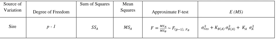
An Analysis of Variance table with all the necessary description
Source of
Variation Degree of Freedom
Sum of Squares Mean
Squares Approximate F-test E (MS)
Sire
p - 1 𝑆𝑆𝐴 𝑀𝑆𝐴 𝐹 =𝑀𝑆𝐴
𝑀𝑆𝜃 ~ 𝐹(𝑝−1), 𝐹𝜃 𝜎𝑟𝑒𝑠
2 + 𝐾
𝐵(𝐴) 𝜎𝐵(𝐴)2 + 𝐾𝐴 𝜎𝐴2
7 8 9 10
3 2
1
1 2 3 4 5 6
1
2 4 5 qi
P
. . .
. . .
. . . nij Figure 1
Table1: ANOVA table for two –stage nested design random effect model
From the table 1, 𝐾𝐴, 𝐾𝐵(𝐴), 𝐾1 , 𝑀𝑆𝜃 , 𝐹𝜃, was derived with the denotations below and approximate F test was derived too since there is no immediate F ratios for the main effects in a case of unbalanced nested design.
𝐾𝐴= 𝑁 − 𝑁−1∑ 𝑁𝑖 𝑖2 ; 𝐾𝐵(𝐴)=
∑ 𝑁𝑖 𝑖2∑ 𝑛𝑖 𝑖𝑗−2 𝑁−1∑ 𝑛𝑖𝑗 𝑖𝑗2
∑ 𝑞𝑖 𝑖−𝑝 ; 𝐾1=
𝑁−∑ 𝑁𝑖 𝑖−1∑ 𝑛𝑖𝑗 𝑖𝑗 2 ∑ 𝑞𝑖 𝑖−𝑝 ;
𝐹𝜃= (𝑀𝑆𝜃)2�𝜃2�𝑀𝑆𝐵(𝐴)�
2
𝐹𝐵 +(1−𝜃)2[𝑀𝑆𝑟𝑒𝑠]𝐹𝑍 �
−1
; 𝑤ℎ𝑒𝑟𝑒 𝜃 = 𝐾𝐵(𝐴)
𝐾1 , 𝛼 = 0.05
𝑎𝑙𝑠𝑜; 𝑀𝑆𝜃= 𝜃𝑀𝑆𝐵(𝐴)+ (1 − 𝜃)𝑀𝑆𝑟𝑒𝑠 ;
𝑤𝑒 𝑎𝑙𝑠𝑜 𝑑𝑒𝑓𝑖𝑛𝑒 𝐹𝑍= 𝑁 − � 𝑞𝑖
𝑖
; 𝐹𝐵= � 𝑞𝑖
𝑖
− 𝑝
𝑆𝑆𝐴 is sum of square of sire; 𝑆𝑆𝐵(𝐴) is the sum of square of dam nested with sire.
𝑆𝑆𝑟𝑒𝑠 is the residual sum of square; 𝑆𝑆𝑇 is the sum of square total.
𝑀𝑆𝐴 is the mean square of sire; 𝑀𝑆𝐵(𝐴) is the mean square of dam nested within sire.
𝑀𝑆𝑟𝑒𝑠 is the mean square of the residual; 𝜎𝑟𝑒𝑠2 is the variance of the residual.
𝜎𝐴2 is the variance of sire; 𝜎𝐵(𝐴)2 is the variance of dam nested within sire.
3.0 Methods of Variance Component Estimation
Estimation of variance components is a method often used in population genetics and applied in animal breeding.
Even experienced population geneticists nowadays feel lost if confronted with the huge set of different methods of
variance component estimation. Especially because there exists no uniformly best method, a decision which method
should be used is often difficult to take, [22]. This work considered only the frequency approach. This approach
assumes that the parameters of the distribution and by this especially the overall mean and the variance components
are fixed but unknown real values or vectors. Quasi Maximum Likelihood Method (QML), Analysis of Variance
Method (ANOVA), Restricted Maximum Likelihood Method (REML), and Maximum Likelihood Method (ML),
Modified Maximum-Likelihood Method (MML) were those five methods of variance components estimation from
the frequency approach, considered in this work. These methods were chosen on no criteria.
3.1
Analysis of Variance Method (ANOVA-method)
According to [10], analysis of variance method is the one of the oldest and commonest methods of estimating
variance components. In this method we replace in the column E (MS) of the ANOVA table the variance
Dam(sire) 𝐹𝐵= � 𝑞𝑖 −𝑝
𝑖
𝑆𝑆𝐵(𝐴) 𝑀𝑆𝐵(𝐴) 𝐹 =𝑀𝑆𝑀𝑆𝐵(𝐴)
𝑟𝑒𝑠 ~ 𝐹𝐹𝐵, 𝐹𝜃 𝜎𝑟𝑒𝑠
2 + 𝐾
1𝜎𝐵(𝐴)2
Residual 𝐹𝑍= 𝑁 − � 𝑞𝑖
𝑖
𝑆𝑆𝑟𝑒𝑠 𝑀𝑆𝑟𝑒𝑠 𝜎𝑟𝑒𝑠2
Total
N – 1 𝑆𝑆𝑇
ISSN 2348 – 7968 components of each 𝜎 (population standard deviation) by its estimate S (sample standard deviation) and we put the
resulting expressions equal to the observed Mean Square component and finally we solve the resulting equations by
substitution. In this case where we considered unbalanced two- stage classification this leads to:
𝑆2= 𝑀𝑆
𝑟𝑒𝑠 (1)
𝑆2+ 𝐾
𝐵(𝐴)𝑆𝐵(𝐴)2 + 𝐾𝐴𝑆𝐴2= 𝑀𝑆𝐴 (2)
𝑆2+ 𝐾
1𝑆𝐵(𝐴)2 = 𝑀𝑆𝐵(𝐴) (3)
On solving equation (1) – (3) above by substitution from the ANOVA table gives
𝑆2= 𝜎�
𝐴𝑁𝑂𝑉𝐴= 𝑀𝑆𝑟𝑒𝑠 (4)
𝑆𝐴2= 𝜎�𝐴. 𝐴𝑁𝑂𝑉𝐴= 𝐾1
𝐴�𝑀𝑆𝐴− 𝑀𝑆𝑟𝑒𝑠− 𝐾𝐵(𝐴)
𝐾1 �𝑀𝑆𝐵(𝐴)− 𝑀𝑆𝑟𝑒𝑠�� (5)
𝑆𝐵(𝐴)2 = 𝜎�𝐵(𝐴).𝐴𝑁𝑂𝑉𝐴= 𝐾11�𝑀𝑆𝐵(𝐴)− 𝑀𝑆𝑟𝑒𝑠� (6)
Therefore, from the computation carried out;
𝑆2= 464.2744, 𝑆
𝐴2= 178.0210 , 𝑎𝑛𝑑 𝑆𝐵(𝐴)2 = 32.4560
3.2
Quasi- Maximum-Likelihood Method (QML)
A quasi-maximum likelihood estimate is obtained by minimizing the likelihood function of the sample under the
restriction that the solution lies in the parameter space. Without this restriction some variance components may be
negative. For more details, see [23]. We estimate the variances using these equations:
𝑆2= 𝜎�
𝑄𝑀𝐿2 = 𝑀𝑆𝑟𝑒𝑠 (7)
𝑆𝐴2= 𝜎�𝐴. 𝑄𝑀𝐿2 =𝐾1𝐴�(𝑝−1)𝑝 𝑀𝑆𝐴− 𝑀𝑆𝑟𝑒𝑠� (8)
𝑆𝐵(𝐴)2 = 𝜎�𝐵(𝐴). 𝑄𝑀𝐿2 =𝐾𝐵(𝐴)1 �𝑦
∗
𝑥∗𝑀𝑆𝐵(𝐴)− 𝑀𝑆𝑟𝑒𝑠� (9)
𝑆2= 464.2743 , 𝑆
𝐴2= 170.6439 , 𝑎𝑛𝑑 𝑆𝐵(𝐴)2 = 32.1370, .
𝑥∗= 𝑁 − � 𝑞
𝑖 𝑖
; 𝑦∗= �𝑁 − � 𝑞
𝑖 𝑖
� − 1 ; 𝑁 = 90; � 𝑞𝑖
𝑖
= 60 ;
𝑝 = 20; 𝑥∗= 31; 𝑦∗= 30
3.3
Maximum Likelihood Method (ML)
According to [14] a real maximum likelihood estimator was derived. The restriction being imposed on it is to enable
the solution to lie within the parameter space. The estimators here are biased. Variances can be computed like:
𝑆2= 𝜎�
𝑀𝐿2 = 𝑀𝑖𝑛 �𝑀𝑆𝑟𝑒𝑠, 𝑆𝑆𝑟𝑒𝑠𝑥+ 𝑆𝑆∗ 𝐴� (10),
𝑤ℎ𝑒𝑟𝑒 𝑥∗ 𝑖𝑠 𝑘𝑛𝑜𝑤𝑛
𝑆𝐴2= 𝜎�𝐴. 𝑀𝐿2 =𝐾1𝐴𝑀𝑎𝑥 ��(𝑝−1)𝑝 𝑀𝑆𝐴− 𝑀𝑆𝑟𝑒𝑠� ; 0� (11)
𝑆𝐵(𝐴)2 = 𝜎�𝐵(𝐴). 𝑀𝐿2 =𝐾𝐵(𝐴)1 𝑀𝑎𝑥 ��𝑦
∗
𝑥∗𝑀𝑆𝐵(𝐴)− 𝑀𝑆𝑟𝑒𝑠� ; 0� (12)
𝑆2= 464.2742, 𝑆
𝐴2= 170.6439 , 𝑎𝑛𝑑 𝑆𝐵(𝐴)2 = 32.1370,
3.4
Restricted Maximum-Likelihood Method (REML)
According to [2], restricted maximum-likelihood uses a translation invariant restricted likelihood function depending
on the variance components to be estimated only and not on the fixed effects like 𝜇 . This restricted likelihood
function as a function of the sufficient statistics for the variance components. The latter is then derived with respect
to the variance components under the restriction that the solutions are non- negative. The solutions are:
𝑆2= 𝜎�
𝑅𝐸𝑀𝐿2 = 𝑀𝑖𝑛 �𝑀𝑆𝑟𝑒𝑠, 𝑆𝑆𝑟𝑒𝑠𝑦+ 𝑆𝑆∗ 𝐴� (13)
𝑤ℎ𝑒𝑟𝑒 𝑦∗ 𝑖𝑠 𝑘𝑛𝑜𝑤𝑛
𝑆𝐴2= 𝜎�𝐴. 𝑅𝐸𝑀𝐿2 =𝐾1𝐴𝑀𝑎𝑥{(𝑀𝑆𝐴− 𝑀𝑆𝑟𝑒𝑠); 0} (14)
𝑆𝐵(𝐴)2 = 𝜎𝐵(𝐴). 𝑅𝐸𝑀𝐿2 =𝐾11𝑀𝑎𝑥��𝑀𝑆𝐵(𝐴)− 𝑀𝑆𝑟𝑒𝑠�; 0� (15)
𝑆2= 464.2741, 𝑆
𝐴2= 184.5122 , 𝑎𝑛𝑑 𝑆𝐵(𝐴)2 = 32.4560.
3.5
Modified Maximum-Likelihood Method (MML)
Details on the estimation processes can be seen in [26] and [16]. Hence the solutions are given as:
𝑆2= 𝜎�
𝑀𝑀𝐿2 = 𝑀𝑖𝑛 �𝑀𝑆𝑟𝑒𝑠 ,𝑆𝑆𝑟𝑒𝑠𝑥∗+1+𝑆𝑆𝐴 ,𝑆𝑆𝑟𝑒𝑠+𝑆𝑆𝐴+𝑥
∗𝑦�2
𝑦∗+2 , … � (16)
𝑆𝐴2= 𝜎�𝐴. 𝑀𝑀𝐿2 =𝐾1𝐴𝑀𝑖𝑛 〈�𝑀𝑎𝑥 ��(𝑃−1)𝑃+1 𝑀𝑆𝑟𝑒𝑠� ; 0�� ; 𝑀𝑎𝑥 ��𝑆𝑆𝐴+𝑥
∗𝑦�2…
𝑥∗+2 − 𝑀𝑆𝑟𝑒𝑠� ; 0�〉 (17)
𝑆𝐵(𝐴)2 = 𝜎�𝐵(𝐴). 𝑀𝑀𝐿2 =𝐾𝐵(𝐴)1 𝑀𝑖𝑛 〈𝑀𝑎𝑥 �� 𝑦
∗
𝑥∗+1𝑀𝑆𝐵(𝐴)− 𝑀𝑆𝑟𝑒𝑠� ; 0� ; 𝑀𝑎𝑥 ��𝑆𝑆𝐵(𝐴)+ 𝑥
∗𝑦�2…−𝑀𝑆𝑟𝑒𝑠
𝑥∗+2 � ; 0�〉 (18)
ISSN 2348 – 7968
𝑆2= 464.2740 , 𝑆
𝐴2= 95.4440 , 𝑎𝑛𝑑 𝑆𝐵(𝐴)2 = 16.6741.
4.0
Evaluation of the Analysis of Variance Table
The calculated values of the parameters in the ANOVA Table were given below. See appendix for details.
𝑆𝑆𝐴= 𝑆𝑆𝑠𝑖𝑟𝑒= 26.349.857; 𝑆𝑆𝐵(𝐴)= 𝑆𝑆𝑑𝑎𝑚(𝑠𝑖𝑟𝑒)= 20, 516.324; 𝑆𝑆𝑇𝑜𝑡𝑎𝑙 = 2,170,418
𝑆𝑆𝑟𝑒𝑠 = 14,392.50; 𝑀𝑆𝑠𝑖𝑟𝑒= 1386.835; 𝑀𝑆𝑑𝑎𝑚(𝑠𝑖𝑟𝑒)= 512.958; 𝑀𝑆𝑟𝑒𝑠= 464.274 𝐾𝐴= 5.0;
𝐾𝐵(𝐴)= 1.0; 𝐾1= 1.5; 𝐹𝜃= 66.00; 𝐹𝑍= 31; 𝐹𝐵= 40
Evaluated Analysis of Variance Table for Two-Stage Nested Design; Unbalanced Case
Source of Variation Degree of Freedom Sum of Squares Mean Square Approximate. - Test Sig-value
Sire 20 26349.857 1386.836 1.660 0.020
Dam(sire) 40 20518.324 512.958 1.690 0.060
Res 31 14392.500 464.274
Total 90 2170418
Table 2: Computed ANOVA table for two stage nested design random effect model.
4.1
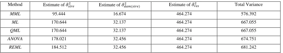
Table of Results
The results of comparative study of different methods of variance components estimation is presented below:
Method Estimate of 𝜎�𝑠𝑖𝑟𝑒2 Estimate of 𝜎�𝑑𝑎𝑚(𝑠𝑖𝑟𝑒)2 Estimate of 𝜎�𝑟𝑒𝑠2 Total Variance
MML 95.444 16.674 464.274 576.392
ML 170.644 32.137 464.274 667.055
QML 170.644 32.137 464.274 667.055
ANOVA 178.021 32.456 464.274 674.751
REML 184.512 32.456 464.274 681.242
Table 3: Comparative table of variance components
Based on the result above, the five different methods of variance components estimation considered from the
frequency approach differ only slightly from one another. But it might be quite different for higher classification or
hierarchy (more than two stage classification) and covariates in the models. Such conclusions can be drawn only if
we apply the different methods to a data set for which the parameter are known like in our collected data. Otherwise
we can only see differences between the methods but we do not know which of them is good. But based on the
results from the numerical example in this study, MML gave the smallest minimum variance among others, and
hence was recommended as the best, among the considered methods from the frequency approach. Moreover, the
effect due to sires is significant whereas that of dams within sire is not.
5.0
Conclusion
In this work where application of two-stage nested design unbalanced case was applied on a population of Gudali
beef Cattle, observing weight of the progeny under dams nested with the sires with a view to observe the significant
effects of variability and the variance components, conclusion was that the variability effects of sires was significant
and that of dams within sire was not. Moreover, modified maximum likelihood method of variance component
estimation was recommended as the one with the smallest minimum variance. This smallest minimum variance,
which Modified maximum likelihood method has placed it first before the other considered methods, in line with the
properties of estimators [22].
Appendixes
App.1Weaning Weight
Sire Dam 1 2 3
1. 1
2 3 189 194 155 180 168
203 145
2. 4
5 6 150 160 170 163 123 131
3. 7
8 9 112 107 146 182 133
4. 10
11 12 163 140 156 130 149 179
5. 13
14 15 149 139 113 109
6. 16
17 18 166 169 150 166 165 150 140
7. 19
20 21 170 139 152 149
8. 22
23 24 202 205 149 164 170
9. 25
26 27 146 160 200 129 167 160
10. 28 29 30
171 170 145
11. 31 32 33 89 128 130 100 144 72
12. 34 35 36
128 224 160
13. 37 38 39
169 146 144
14. 40 41 42
113 169 187
15. 43 44 45 149 150 198 168 139
16. 46 47
140 163
48 180
17. 49 50 51
120 145 113
18. 52 53 54
139 143 157
19. 55 56 57 166 149 126 142
20. 58 59 60 163 159 163 150
App. Table 1: table showing the weaning weight of progeny produced by dams nested within sire.
App.2
Dam
𝑛𝑖𝑗2
Sire 1 2 3
1. 4 4 9 17
2. 4 4 4 12
3. 1 4 4 9
4. 4 4 4 12
5. 4 1 1 6
6. 9 4 4 17
7. 4 1 1 6
8. 4 1 4 9
9. 4 4 4 12
10. 9 1 4 14
11. 1 4 4 9
12. 1 1 1 3
13. 1 1 4 6
14. 4 1 1 6
15. 1 4 1 6
16. 1 1 1 3
17. 1 1 1 3
18. 1 1 1 3
19. 1 4 1 6
20. 4 1 1 6
Table 2: 𝑛𝑖𝑗2table.
Calculation of sum of squares
𝑆𝑆𝜇=𝑌…2𝑁= 2109157.319
𝑆𝑆𝐴= � 𝑌𝑖𝑗.2 𝑛𝑖𝑗
𝑖𝑗
−𝑌𝑁 = 26349.857…2
𝑆𝑆𝐵(𝐴)= � 𝑌𝑖𝑗.2 𝑛𝑖𝑗
𝑖𝑗
− �𝑌𝑖..2
𝑁𝑖 𝑛𝑖𝑗
𝑖
= 20516.324
𝑆𝑆𝑇= � 𝑌𝑖𝑗𝑘 2 𝑛𝑖𝑗
𝑖𝑗
= 2170418
𝑆𝑆𝜀= 𝑆𝑆𝑇− 𝑆𝑆𝜇− 𝑆𝑆𝐴− 𝑆𝑆𝐵(𝐴)= 14392.50
Estimation of 𝑲𝑨, 𝑲𝑩(𝑨), 𝑲𝟏,
𝐾𝐴= 𝑁 − 𝑁−1� 𝑁𝑖2 𝑛𝑖𝑗
𝑖
= 4.525 ≈ 5.0
𝐾𝐵(𝐴)=
∑ 𝑁−1∑ 𝑛
𝑖𝑗 2 𝑛𝑖𝑗
𝑖𝑗 − 𝑁−1
𝑛𝑖𝑗
𝑖 ∑ 𝑛𝑛𝑖𝑗 𝑖𝑗2
∑ 𝑞𝑛𝑖𝑖𝑗 𝑖− 𝑝
= 0.74846 ≈ 1.0
𝐾1=
𝑁−1∑ 𝑁
𝑖−1 𝑛𝑖𝑗
𝑖 ∑ 𝑛𝑛𝑖𝑗𝑖𝑗 𝑖𝑗2
∑ 𝑞𝑛𝑖𝑖𝑗 𝑖− 𝑝
= 1.48286 ≈ 1.5
Estimation of 𝑭𝜽
𝐹𝜃= (𝑀𝑆𝜃)2�𝜃2�𝑀𝑆𝐹𝐵(𝐴)� 𝐵
2
+(1 − 𝜃)2[𝑀𝑆𝜀]
𝐹𝑍 �
2
= 66.1365 ≈ 66.0
𝑀𝑆𝜃= 𝜃𝑀𝑆𝐵(𝐴)+ (1 − 𝜃)𝑀𝑆𝜀 = 496.892
Where 𝜃 = 𝐾𝐵(𝐴)𝐾
1 = 0.6
Acknowledgement
The authors are grateful to the Institute of Agricultural Research for Development (IARD), Wakwa Station in
Cameroon, and Dr (Mrs.) H. Foleng, for making the data for this research available.
REFRENCES
[1] Alwin, D. F. (1976). Attitude scales as cogeneric tests: a re-exam1nation of an attitude-behavior model.
Sociometry 39, 377-383.
[2] Anderson, R. L., and Bancroft, T. A. (1952): Statistical Theory in Research. McGraw-Hill, New York.
[3] Bainbridge, T. R. (1965). Staggered nested designs for estimating variance components. Industrial Quality
Control, 22, 12 – 20.
[4] Bush, N. (1971). Unmodeled error analysis on trajectory and orbital estimation. Technometrics 13, 303-314.
[5] Chakravarti, S. R. and Grizzle, J. E. (1975). Analysis of data from multiclinic experiments. Biometrics 31,
325-338.
[6] Crump, S. L. (1946). The estimation of variance components in analysis of variance. Biometrics Bulletin 2, 7-11.
[7] Daniels, H. E. (1939). The estimation of components of variance. J. Roy. Statist. Soc. Suppl. 6, 186-197
[8] Duncan, D. B. and Horn, S. D. (1972). Linear dynamic recursive estimation from the viewpoint of regression
analysis. J· Am. Stat. Assoc. 67, 815-821.
[9] Eisenhart, C. (1947). The assumptions underlying the analysis of variance. Biometrics 3, 1-21.
[10] Fisher, R. A. (1925): Statistical Methods for Research Workers, Oliver and Boyd, London.
[11] Ganguli, M. (1941). A note on nested sampling. Sankya 5, 449-452.
[12] Harville, D. A. (1977). Maximum likelihood approaches to variance component estimation and to related
problems. J. Am. Stat. Assoc. 72 (in press).
[13] Hazel, L. N. and Terrill, C. E. (1945). Heritability of weaning weight and staple length in range Rambouillet
lambs. J. Animal Sci. 4, 347-358.
[14] Herbach, L. H. (1959): Properties of Model II type analysis of Variance tests A: Optimum nature of the F-test
for model II in balanced case. Ann. Math. Statist. 30, 939-959.
[15] Houthakker, H. S., Verleger, P. K., Jr., and Sheehan, D. P. (1974). Dynamic demand analyses for gasoline and
residential electricity. American J· of Agric. Econ. 56, 412-418.
[16] Klotz, J. H., Milton, R. C., and Zacks, S. (1969): Mean Square efficiency of estimators of variance
components. J. Am. Stat. Assoc., 46, 1383-1402.
[17] Lamar, J. M. and Zirk, W. E. (1991). Nested designs in the chemical industry. In Annual Quality Congress
Transactions, American Society for Quality Control, Milwaukee, W. I. pp. 615-622.
[18] Liu, S. and Batson, R. G. (2003). A nested experiment design for gauge gain in steel tube manufacturing.
Quality Engineering. 16(2), 269-282.
[19] Pignatiello, J. (1984). Two stage nested design. ASQC Statistics Division Newsletter, 6(1), September. (This
can be accessed by ASQC members at
31TU
http://www.asq.org/forum/statistical/newsletters/vol_6_no_1_sept 1984.pdfU31T.)
[20] Randall, J. J. (1976). The diallel cross. Unpublished M.S. thesis, Biometrics Unit, Cornell University, Ithaca,
New York.
[21] Rao, C. R. and Kleffe, J. (1988). Estimation of variance components and applications. Amsterdam: North –
Holland.
[22] Rasch, D. and Masata, O. (2006). Methods of variance components estimation. Czech J. Anim. Sci., 51,
2006(6): 227-235.
[23] Rasch, D., Verdooren, L. R., Gowers, J. I. (1999). Fundamentals in the Design and Analysis of Experiments
and Surveys-Grundlagen der planung und Auswertung von Versuchen und Erheungen. Oldenbourg
Verlag, Munchen, Wien.
[24] Satterthwaite, F. E. (1946). An approximate distribution of estimates of variance components. Biometrics
Bulletin 2, 110-114.
[25] Sinibaldi, F. J. (1983). Nested designs in process variation studies. In ASQC Annual Quality Congress
Transaction. Pp. 503 -508. American Society for Quality Control, Milwaukee, W. I.
[26] Stein, C. (1969). Inadmissibility of the usual estimator for the variance of a normal distribution with unknown
mean. Ann. Inst. Statist. Math. (Japan), 16, 155-160.
[27] Vander Heyden, Y., K. De Braekeleer, Y. Zhu, E. Roets, J. Hoogmartens, J. De Beer, and D. L. Massart (1999).
Nested designs in ruggedness testing. Journal of Pharmaceutical and Biomedical Analysis, 20(6), 875
– 887.
[28] Winsor, C. P. and G. L. Clarke (1940). Statistical study of variation in the catch of plankton nets. Sears
Foundation Journal of MarineResearch 3, 1-34.
[29] Yates, F. (1967). A fresh look at the basic principles of the design and analysis of experiments. Proc. 5th
Berkeley Symp. Math. Statist. Prob. IV, 777-790. L. Lecam and J. Neyman, Eds., University of
California Press.