Decision Support
Implementing stochastic multicriteria acceptability analysis
Tommi Tervonen
a,b,c,*, Risto Lahdelma
aa
University of Turku, Department of Information Technology, FIN-20520 Turku, Finland b
INESC—Coimbra, R. Antero de Quental 199, 3000-033 Coimbra, Portugal c
Faculdade de Economia da Universidade de Coimbra, Av. Dias da Silva 165, 3004-512 Coimbra, Portugal Received 27 July 2004; accepted 29 December 2005
Available online 17 April 2006
Abstract
Stochastic multicriteria acceptability analysis (SMAA) is a family of methods for aiding multicriteria group decision making in problems with inaccurate, uncertain, or missing information. These methods are based on exploring the weight space in order to describe the preferences that make each alternative the most preferred one, or that would give a certain rank for a specific alternative. The main results of the analysis are rank acceptability indices, central weight vectors and confidence factors for different alternatives. The rank acceptability indices describe the variety of different preferences resulting in a certain rank for an alternative, the central weight vectors represent the typical preferences favouring each alternative, and the confidence factors measure whether the criteria measurements are sufficiently accurate for making an informed decision.
The computations in SMAA require the evaluation of multidimensional integrals that must in practice be computed numerically. In this paper we present efficient methods for performing the computations through Monte Carlo simulation, analyze the complexity, and assess the accuracy of the presented algorithms. We also test the efficiency of these methods empirically. Based on the tests, the implementation is fast enough to analyze typical-sized discrete problems interactively within seconds. Due to almost linear time complexity, the method is also suitable for analysing very large decision prob-lems, for example, discrete approximations of continuous decision problems.
2006 Elsevier B.V. All rights reserved.
Keywords: Stochastic multicriteria acceptability analysis; Simulation; Multiple criteria analysis; Complexity analysis
1. Introduction
Stochastic multicriteria acceptability analysis (SMAA) methods have been developed for discrete
multicriteria decision aiding (MCDA) problems, where criteria measurements are uncertain or inac-curate and where it is for some reason difficult to obtain accurate or any preference information from the decision makers (DMs) (Lahdelma and Salmi-nen, 2001).
Usually in MCDA problems the preference infor-mation is modelled by determining importance weights for criteria. The SMAA methods are based on exploring the weight space in order to describe
0377-2217/$ - see front matter 2006 Elsevier B.V. All rights reserved. doi:10.1016/j.ejor.2005.12.037
* Corresponding author. Address: INESC—Coimbra, R. Ante-ro de Quental 199, 3000-033 Coimbra, Portugal. Tel.: +351 96 529 1325; fax: +351 23 982 4692.
E-mail addresses: [email protected].fi (T. Tervonen),
[email protected].fi(R. Lahdelma).
the preferences that would make each alternative the most preferred one, or that would give a certain rank for a specific alternative. The main results of the analysis are rank acceptability indices, central weight vectors and confidence factors for different alternatives. The rank acceptability indices describe the variety of different preferences resulting in a cer-tain rank for an alternative, the central weight vec-tors represent the typical preferences favouring each alternative, and the confidence factors measure whether the criteria measurements are sufficiently accurate for making an informed decision.
In MCDA literature outside SMAA, there is a long history of methodologies that allow decision aiding under uncertain and/or imprecise informa-tion. See e.g. Dias and Clı´maco (2000), Dias et al. (2002), Fishburn (1965), Hazen (1986), Kirkwood and Sarin (1985), Mousseau et al. (2000, 2003), and for more general information on this subject, see Figueira et al. (2005). Although this area has been studied for three decades, the SMAA methods are the first ones allowing both preference informa-tion and criteria measurements to be expressed as arbitrarily distributed stochastic variables. The SMAA approach has also recently been applied to extend other MCDA methods to allow using them with imprecise information (see Tervonen et al., 2005).
The SMAA methods are based on inverse weight space analysis, which has also been considered in the works of Charnetski Soland (1978) and Bana e Costa (1986). In the original SMAA method by Lahdelma et al. (1998) the weight space analysis is performed based on an additive utility or value function and stochastic criteria measurements. The SMAA-2 method (Lahdelma and Salminen, 2001) generalized the analysis to a general utility or value function, to include various kinds of preference information and to consider holistically all ranks. The SMAA-3 method (Lahdelma and Salminen, 2002) applies ELECTRE III type pseudo-criteria in the analysis. The SMAA-O method (Lahdelma et al., 2003) extends SMAA-2 for treating mixed ordinal and cardinal criteria in a comparable man-ner. The SMAA-A method (or Ref-SMAA method) models the preferences using reference points and achievement scalarizing functions (Lahdelma et al., 2005).Durbach (2006)has also developed a variant
of the SMAA-A method using achievement
functions.
SMAA methods are applicable in many real-life problem types for a number of reasons. Firstly,
the inverse weight space approach is suitable for many group decision-making problems, where the DMs are unable or unwilling to provide preference information, or it is difficult to reach consensus over the preferences. In such cases the preference infor-mation can be expressed as weight intervals includ-ing preferences of all DMs, or with some other weight distribution accepted by all DMs. SMAA can then be used to compute descriptive informa-tion about the acceptability of different alternatives, and this can help the DMs to identify commonly acceptable compromise solutions. Secondly, SMAA supports a very general and flexible way to model different kinds of uncertain or inaccurate preference and criteria information through stochastic distri-butions. Thirdly, as demonstrated in this paper, the SMAA computations can be implemented very efficiently through numerical methods, making it possible to use the method in many different deci-sion-making contexts, including interactive decision processes. As a consequence, SMAA methods have been successfully applied in a number of real-life decision problems in Finland. For applications of SMAA, see e.g. Hokkanen et al. (1998, 1999, 2000), Kangas et al. (2003, in press), Kangas and Kangas (2003), Lahdelma and Salminen (2006), Lahdelma et al. (2001, 2002).
In this paper we describe how the basic computa-tions of the SMAA-2 and SMAA-O methods can be implemented efficiently through Monte Carlo simu-lation. We have chosen to present the computations of these two methods, because they form the basis for all other SMAA variants. In particular, we pres-ent the algorithms for computing the rank accept-ability indices, central weight vectors, and confidence factors. We begin by introducing the SMAA-2 and SMAA-O methods in Section 2. In Section 3, we describe the implementation of the algorithms and discuss techniques for handling pref-erence information. Following this, we analyze the complexity of the algorithms theoretically in Section 4. We assess the accuracy of the computations in Section 5, and present results from empirical effi-ciency tests in Section 6. We end this paper with conclusions in Section7.
2. The SMAA-2 and SMAA-O methods 2.1. The basic SMAA-2 method
The SMAA-2 method (Lahdelma and Salminen, 2001) has been developed for discrete stochastic
multicriteria decision-making problems with multi-ple DMs. SMAA-2 applies inverse weight space analysis to describe for each alternative what kind of preferences make it the most preferred one, or place it on any particular rank. The decision prob-lem is represented as a set of m alternatives {x1,x2,. . .,xm} that are evaluated in terms ofn cri-teria. The DMs’ preference structure is represented by a real-valued utility or value function u(xi,w). The value function maps the different alternatives to real values by using a weight vectorwto quantify DMs’ subjective preferences. SMAA-2 has been developed for situations where neither criteria mea-surements nor weights are precisely known. Uncer-tain or imprecise criteria are represented by stochastic variables nij with joint density function
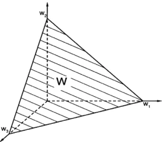
fX(n) in the space XRm·n. The DMs’ unknown or partially known preferences are represented by a weight distribution with joint density function fW(w) in the feasible weight spaceW. Total lack of preference information is represented in ‘Bayesian’ spirit by a uniform weight distribution in W, that is, fW(w) = 1/vol(W). The weight space can be defined according to needs, but typically, the weights are non-negative and normalized, that is; the weight space is an n1-dimensional simplex inn-dimensional space: W ¼ w2Rn: wP0 and X n j¼1 wj¼1 ( ) . ð1Þ
Fig. 1presents the feasible weight space of a three-criterion problem as the shaded triangle with corner points (1, 0, 0), (0, 1, 0), and (0, 0, 1).
The value function is used to map the stochastic criteria and weight distributions into value distribu-tions u(ni,w). Based on the value distributions, the rank of each alternative is defined as an integer from the best rank (=1) to the worst rank (=m) by means of a ranking function
rankði;n;wÞ ¼1þX m
k¼1
qðuðnk;wÞ>uðni;wÞÞ; ð2Þ
whereq(true) = 1 andq(false) = 0. SMAA-2 is then based on analysing the stochastic sets of favourable rank weights
WriðnÞ ¼ fw2W :rankði;n;wÞ ¼rg. ð3Þ
Any weightw2Wr
iðnÞresults in such values for
dif-ferent alternatives, that alternativexiobtains rankr. The first descriptive measure of SMAA-2 is the rank acceptability indexbri, which measures the vari-ety of different preferences (weights) that grant alternative xi rank r. It is the share of all feasible weights that make the alternative acceptable for a particular rank, and it is most conveniently expressed percentage-wise. The rank acceptability indexbri is computed numerically as a multidimen-sional integral over the criteria distributions and the favourable rank weights as
bri ¼ Z n2X fXðnÞ Z w2Wr iðnÞ fWðwÞdwdn. ð4Þ
The most acceptable (best) alternatives are those with high acceptabilities for the best ranks. Evi-dently, the rank acceptability indices are in the range [0, 1], where 0 indicates that the alternative will never obtain a given rank and 1 indicates that it will obtain the given rank always with any choice of weights.
Favourable rank weights and rank acceptability indices are illustrated inFig. 2. The figure represents a deterministic two-criterion, three-alternative prob-lem with linear value function. The favourable first rank weightsðW1iÞare shown in light gray, bordered by the favourable second rank weightsðW2iÞin dark gray. First and second rank acceptability indices
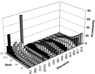
ðb1i;b2iÞ correspond in this figure to the distances spanned by the favourable rank weights. When the problem contains multiple criteria and alternatives, the rank acceptability indices can be better visual-ized by a three-dimensional column chart. Fig. 3 shows the rank acceptability indices from the Hel-sinki Harbour case with 13 alternatives and 11 crite-ria (Hokkanen et al., 1999).
The first rank acceptability index b1i is called the acceptability index ai. The acceptability index is par-ticularly interesting, because it is non-zero for sto-chastically efficient alternatives (alternatives that are efficient with some values for the stochastic cri-teria measurements) and zero for inefficient alterna-tives. The acceptability index not only identifies the efficient alternatives, but also measures the strength of the efficiency considering the uncertainty in crite-ria and DMs’ preferences.
Thecentral weight vectorwc
i is the expected centre
of gravity (centroid) of the favourable first rank weights of an alternative. The central weight vector
represents the preferences of a ‘typical’ DM sup-porting this alternative. The central weights of dif-ferent alternatives can be presented to the DMs in order to help them understand how different weights correspond to different choices with the assumed preference model. The central weight vector wc
i is
computed numerically as a multidimensional inte-gral over the criteria distributions and the favour-able first rank weights using
wci ¼ Z n2X fXðnÞ Z w2W1 iðnÞ fWðwÞwdwdn=ai. ð5Þ
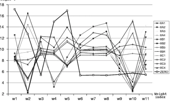
Fig. 4presents a sample chart of central weight vec-tors from the Helsinki Harbour decision-making problem.
Theconfidence factorpc
i is the probability for an
alternative to obtain the first rank when the central weight vector is chosen. The confidence factor is computed as a multidimensional integral over the criteria distributions using
pc i ¼ Z n2X:rankði;n;wc iÞ¼1 fXðnÞdn. ð6Þ
Confidence factors can similarly be calculated for any given weight vectors. The confidence factors measure whether the criteria measurements are accurate enough to discern the efficient alternatives. 2.2. Ordinal criteria
The SMAA-O method (Lahdelma et al., 2003) extends SMAA-2 to handle ordinal criteria mea-surements. In SMAA-O, the criteria may be ordinal, cardinal, or mixed. In the mixed case some of the criteria are measured on cardinal (interval) scales and others on ordinal scales. For an ordinal crite-rion, each alternative is measured by assigning it a rank level. The rank levelxijis an integer from the best rank level 1 to the worst rank levelmj. Observe that multiple alternatives may obtain the same rank level, in which casemj<m. The idea in SMAA-O is to map the ordinal criteria measurements into cardi-nal scales before they are used in the computations. The mapping is implemented by a functiongj(Æ) that preserves the ordinal information:
xijxkj()gjðxijÞ>gjðxkjÞ 8i;k2 f1;. . .;mg. ð7Þ
Without loss of generality we can assume that the mapping is scaled to interval [0, 1]. Otherwise the
Fig. 2. First and second rank acceptabilities in a deterministic two-criterion problem with linear value function (Lahdelma and Salminen, 2001).
Fig. 3. Rank acceptability indices (bi) from the Helsinki Harbour
shape of the mapping is unknown. SMAA-O simu-lates numerically all such mappings that preserve the ordinal criteria information.
2.3. Preference information
There are several different ways to handle partial preference information in SMAA methods. In this paper we focus on two ways that are applicable when the value function is additive (Lahdelma and Salminen, 2001):
• interval constraints for weights, and • complete ranking of the criteria.
The preference information might also be mixed: there might be exact numerical values for some weights, ranking for a set of weights, and interval constraints for some weights. Mixed preference information is not considered in this paper.
Interval constraints for weights are given in the form
06wmin
j 6wj6wmaxj 61; wherej2 f1;. . .;ng. ð8Þ
The intervals [wmin,wmax] can be defined so that they contain the preferences of the DMs (and other inter-est groups). The DMs can express their preferences
either as precise weights or as weight intervals. The weight space analysis of SMAA is then performed in the restricted weight space
W0¼ fw2Wjwminj 6wj6wmax
j ; j¼1;. . .;ng. ð9Þ
This means that the uniform weight distribution fW(w) is redefined as fWðwÞ ¼ 1=volðW0Þ if w2W0; 0 otherwise. ( ð10Þ
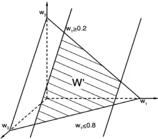
Fig. 5illustrates the restricted feasible weight space of a three-criterion problem with lower and upper bounds forw1.
Complete ranking of the criteria is expressed as a sequence of inequality constraints for the weights
wj1Pwj2 P Pwjn. ð11Þ
Such a ranking can be obtained by asking the DMs to identify the most important, second most tant, etc. criterion. When judging mutual impor-tance of the criteria, the DMs should consider the difference between the best and worst value for each criterion. If the DMs consider two criteria equally important, this can be represented by an equality constraint between those criteria in(11).Fig. 6 illus-trates the feasible weight space for a three-criterion problem with the rankingw1Pw2Pw3.
3. Description of the SMAA algorithm
The multidimensional integrals(4)–(6)of SMAA computations are in practice impossible to compute analytically, because the distributions fX and fW vary according to the application and can be arbi-trarily complex. Straightforward integration tech-niques based on discretizing the distributions with respect to each dimension are infeasible, because the integrals have a very high dimension, and the required effort depends exponentially on the num-ber of dimensions. For example, in a problem with
eight criteria and 10 alternatives, the dimension of the integral for computing rank acceptability indices is 88, because in(4)the outer integration is through the eight-dimensional criteria space, and the inner one through the space of all criteria measurements for all alternatives (8·10 = 80 dimensions). How-ever, due to the nature of the problem, we do not need an answer with very high precision. Monte Carlo simulation is a well-established method for computing approximative values for high-dimen-sional integrals. In Monte Carlo simulation the required number of iterations is inversely propor-tional to the square of the desired accuracy, but does not significantly depend on the dimensionality of the problem (Fishman, 1996). Thus, Monte Carlo simulation can be used to obtain a precision of a few decimal places with moderate effort.
The algorithm is described in four parts. We first describe the method for generating a criterion matrix with cardinal and ordinal criteria. Secondly, we describe the applied weight generation technique and how preference information is handled. Before we describe the actual SMAA algorithm, we observe that the confidence factors(6) depend both on the central weight vectors and on the acceptability indi-ces. As a consequence, the algorithm must consist of two phases.Phase 1consists of computation of the rank acceptability indices and the central weight vectors. The confidence factors are computed in Phase 2.
The following symbols are used inAlgorithms 1– 4:
hji number of times alternative i is evaluated into rank jin Monte Carlo simulations of Phase 1 (hits for rankjof alternativei) Kw number of iterations in Phase 1 (rank
acceptability index and central weight vec-tor computation)
Kc number of iterations in Phase 2 (confidence
factor computation)
mj number of rank levels for ordinal criterionj
r= [r1,. . .,rm] vector of ranks of the alternatives
t= [t1,. . .,tm] vector of value function values of the alternatives
The algorithms also use the following functions and subroutines:
RANDU[0,1]() function returning a uniformly
dis-tributed random number from the interval [0, 1]
RANDX() function returning a random criterion matrix from criteria distributionfX
Fig. 6. Feasible weight space of a three-criterion problem with ranking of the criteria.
Fig. 5. Feasible weight space of a three-criterion problem with lower and upper bounds forw1.
RANDW() function returning a random weight vector from weight distributionfW
RANK(t) function returning a vector of ranks cor-responding to the vector of value function valuest
SORTasc(s) subroutine sorting the components of
vectorsinto ascending order
SORTdesc(s) subroutine sorting the components of
vectorsinto descending order
3.1. Generation of the criteria measurement matrix The RANDX() function generates a random cri-terion matrix of size m·n from the given criteria distribution. Each row of the matrix contains crite-ria measurements of a certain alternative. Cardinal criteria measurements follow a joint distribution, or independent distributions. We do not consider joint distribution for cardinal criteria in this paper. Refer toLahdelma et al. (2004). Independent crite-ria measurements are generated separately from their corresponding distributions. Their distribu-tions may have an arbitrary shape (e.g.uniform, normal,. . .).
If some of the criteria are measured on ordinal scales, then the ordinal to cardinal mapping must be simulated for those criteria each time a new cri-terion matrix is created. The ordinal to cardinal mapping is simulated using the following method: first,mj2 uniformly distributed random numbers from the interval ]0, 1[ are generated and sorted into
descending order (mjis the number of rank levels). Then, 1 is inserted as the first number and 0 as the last number. The simulated cardinal value for rank leveljis then thejth of these numbers. Thus the sim-ulated cardinal value for the best rank level is 1, and the simulated cardinal value for the worst rank level is 0. The simulated cardinal values for other rank levels should be unique and in the interval ]0, 1[. Because the majority of pseudo-random number generators will not produce duplicate floating point values except after a very long sequence, it is in practice unnecessary to have any special treatment for duplicate values. The procedure for generating the simulated cardinal values is defined as pseudo-code in Algorithm 1. Complexity of this procedure is due to sorting O(mlog(m)). The procedure must be executed once for each ordinal criterion when a new criterion matrix is generated. Fig. 7illustrates a possible mapping with 11 rank levels generated by this procedure.
Algorithm 1. Generation of mj simulated cardinal values (q1,. . .,qmj). Output:q 1:forj 2tomj1 do 2: qj RANDU[0,1]() 3:end for 4: SORTdesc(q) 5:q1 1 6:qmj 0
3.2. Generation of weights and handling preference information
The RANDW() function generates the weights from the given weight distribution. We describe weight generation corresponding to three different types of preference information:
• absent preference information, • interval constraints for weights, and • complete ranking of the criteria.
In case of absent preference information the weights are generated from a uniform distribution in the normalized weight space (1). Because the weights must sum to unity, thenweightswjare gen-erated according to the following method: firstn1 independent random numbers are generated from the uniform distribution in interval [0, 1], and sorted into ascending order (q1,q2,. . .,qn1). After that, 1
is inserted as the last number (qn= 1) and 0 as the first number (q0= 0). Uniformly distributed
nor-malized weights are then obtained as intervals between the consecutive numbers (wj=qjqj1)
(David, 1970). The procedure for generating the n uniformly distributed normalized weights is defined in Algorithm 2. Complexity of this procedure is O(nlog(n)) due to sorting.
When preference information is available, the weight generation process must be modified a little. Upper and lower bounds for weights (and in princi-ple also more comprinci-plex weight constraints) can be implemented by the rejection technique. After a vec-tor of uniformly distributed normalized weights has been generated, the weights are tested against their bounds. If any of the constraints is not satisfied, the entire set is rejected and the weight generation is repeated. A problem with the rejection technique is that it may cause a very large share of the weights to be rejected and a very small share of them to be accepted. A small acceptance rate not only slows down the computation, but may also cause problems with the quality of the generated pseudo-random numbers that pass the rejection test. However, upper and lower bounds affect the acceptance rate differ-ently. As can be seen fromFig. 5, upper bounds cut off the tip of the simplex, but lower bounds cut off the base. In a high-dimensional weight space, the vol-ume of the tip is very small, but the volvol-ume of the base is large in relation to the entire weight space.
To estimate how large a share of the weight vec-tors need to be rejected due to upper bounds, we
assume that all weights have a common upper bound wmax. Then the probability for the largest of the generated weights to exceed the upper bound is P½maxfwjg>wmax ¼nð1wmaxÞn1 n 2 ð12w maxÞn1 þ ð1Þk1 n k ð1kw maxÞn1 ; ð12Þ
where the series continues as long as 1kwmax> 0 (David, 1970). For example, if there are n= 5 weights with upper boundwmax= 0.4, the rejection percentage is 63.2%. If we are applying both lower and upper bounds, it might be the case, that the lower bounds render some upper bounds redun-dant. Consider a three-criterion case with a lower bound of 0.3 for all weights. Then the maximum value that any weight may obtain is 10.30.3 = 0.4. Therefore all upper bound weight constraints of 0.4 or higher are redundant.
The rejection technique can be very inefficient for weights with lower bounds in high-dimen-sional problems. Lower bounds can be treated effi-ciently by using a simple transformation technique. With lower bounds the feasible weight space becomes W0¼ w2Rnjw jPwminj and Xn j¼1 wj¼1 ( ) ; ð13Þ
which has the same simplex shape as the original weight space W, but is smaller. By substituting
w0j¼wjwminj the restricted weight space becomes
W0¼ w02Rnjw0 jP0 and Xn j¼1 w0j¼1C ( ) ; whereC¼X n j¼1 wminj . ð14Þ
The shifted weights w0j can now be generated by a modification of Algorithm 2where the weights are generated to sum to 1C instead of 1. Then the lower bounded weightswjare obtained by substitut-ing backwj¼w0jþw
min
j . Lower bounds do therefore
not increase the complexity of weight generation. Preference information presented in form of a complete ranking of the criteria is handled using a similar technique that was used for simulating the
ordinal to cardinal mapping in the previous section. First we generate a set of weights from a uniform distribution in the normalized weight space as in the case of absent preference information. Then we sort the weights into a consistent order according to the ranking of the criteria. This does not increase the complexity of weight generation.
Algorithm 2. Generation ofnuniformly distributed random weights from the interval [0, 1] (w1,. . .,wn) which sum to unity.
3.3. Phase 1. Computation ofbr i and w
c i
To compute the rank acceptability indicesbri and the central weight vectorswc
i for each alternativei,
we must integrate over the criteria and weight distri-butions. Straightforward computation of the rank acceptability indices (4) would require executing Monte Carlo simulation mÆn times, once for each index. Similarly, computing the central weight vec-tor(5) for each alternative would requirem
execu-tions. We can speed up the computation
remarkably by observing that all rank acceptability indices and central weight vectors can be computed in a single simulation run. To do this, we generate during each iteration a random criterion matrix and a random weight vector from their correspond-ing distributions. Then we compute statistics on the ranks that different alternatives obtained and update the central weight vector of the most pre-ferred alternative. Phase 1 is described as pseudo-code inAlgorithm 3.
Algorithm 3 uses the function RANK(t). RANK(t) returns a vector of ranks for alternatives based on their values in vector t. For example, if t= [0, 0.5, 0.2], the resulting rank vector is [3, 1, 2]. This function is implemented efficiently by sorting
the alternatives into descending order by their val-ues and then assigning consecutive ranks from 1 to m to the sorted alternatives. Sometimes two or more alternatives may have the same values, and they should thus be assigned the same rank. Rank assignment should be implemented to handle such cases properly. However, shared ranks will be extre-mely rare when the criteria measurements are sto-chastic and independent. Complexity of this procedure is due to sorting O(mlog(m)).
Observe in Algorithm 3 that the central weight vector ðwc
iÞ is defined only when the acceptability
index is non-zero, or, equivalently, when hits for the first rank ðh1iÞis greater than zero.
Algorithm 3. Monte Carlo simulation to compute the central weight vectors (wci’s) and the acceptabil-ity indices (bri’s). Output:w 1:forj 1to n1 do 2: qj RANDU[0,1]() 3:end for 4: SORTasc(q) 5:q0 0 6:qn 1 7:forj 1to ndo 8: wj qjqj1 9:end for Output:wc i’s,b r i’s 1: // Initialization ofwc
i and hit count
2:fori 1tomdo 3: wc i 0 4: forj 1 tomdo 5: hji 0 6: end for 7:end for 8: // Main loop 9:fork 1 toKwdo 10: w RANDW() 11: x RANDX() 12: fori 1to mdo 13: ti u(xi,w) 14: end for 15: r RANK(t) 16: fori 1to mdo 17: hrii hrii þ1 18: ifri= 1then 19: wc i w c i þw 20: end if 21: end for 22:end for 23: // Computation ofwc i andb r i 24:for i 1 tomdo 25: ifh1i >0 then 26: wc i w c i=h 1 i 27: end if 28: forj 1to mdo 29: bji hji=Kw 30: end for 31:end for
3.4. Phase 2. Computation ofpc i
To compute the confidence factorspc
i from(6)we
must integrate over the criteria distribution with respect to the different central weight vectors. Naive implementation of the computation would require repeating the simulation m times, once for each alternative. Again, we can device a way to compute all integrals simultaneously. To do this, we first gen-erate during each iteration a random criterion matrix from the appropriate criteria distribution. After that, we evaluate for each alternative whether that alternative is the most preferred one using its central weight vector and the random criterion matrix. This technique decreases the number of generated criterion matrices by a factor of m. However, to evaluate if the alternative is the most preferred one, we still need to evaluate the value function a maximum of m times in an inner loop. We shall see later a surprising result on the expected complexity of this algorithm. The algo-rithm for Phase 2 is presented as pseudo-code in Algorithm 4.
Algorithm 4. Monte Carlo simulation to compute the confidence factors (pci’s).
4. Complexity of the SMAA algorithm
If all of the criteria are measured on cardinal scales, the complexity of the algorithm for Phase 1 (Algorithm 3) is O(KwÆ/W+KwÆ/X+KwÆmÆn+ KwÆmlog(m) +m2), where /Wis the complexity of generating a weight vector from the weight distribu-tion and/Xis the complexity of generating a crite-rion matrix from the criteria distribution. In many applications the weights are generated from a uni-form distribution following the method described before (Algorithm 2). In practice the number of iter-ationsKwm, because Kwis fairly large (104–106)
to obtain sufficient accuracy and mis fairly small. With these assumptions the complexity can be writ-ten as O(KwÆ(nlog(n) +mÆn+/X+ mlog(m))). If criteria measurements are independent, the com-plexity is O(KwÆ(n log(n) +mÆn+ mlog(m))). In
many practical decision-making problems the term mÆn dominates, and the complexity can thus be written as O(KwÆmÆn). If some of the criteria are
measured on ordinal scales, the ordinal to cardinal mapping is required for those criteria, and in that case the total complexity of Algorithm 2 is O(KwÆnÆmlog(m)).
The complexity of the algorithm for Phase 2 (Algorithm 4) is O(KcÆ(/X+m2Æn)), if all of the criteria are measured on cardinal scales. During each iteration, the algorithm first generates a crite-rion matrix for all alternatives, and then uses these when computing the values with different central weight vectors. This decreases the number of crite-rion matrices generated during Phase 2 of the algo-rithm fromKcÆmtoKcand affects the running time
remarkably. If the criteria measurements are inde-pendent, the complexity of the algorithm for Phase 2 can be written as O(KcÆm2Æn).
The algorithm for Phase 2 which has squared worst-case complexity with respect tom, has in fact quite low typical-case complexity. The squared complexity is a consequence of the inner loop com-paring values of the alternatives. However, that loop is almost never executed completely. Normally, when the criteria measurements are independent stochastic variables, the values of the alternatives will be distinct. If we assume that during each Monte Carlo iteration one of the alternatives will have the best value with respect to its central weight vector, one the second best, etc., and if the alterna-tives are compared in a random order, then the Output:pc i’s 1:fori 1 tomdo 2: pc i 0 3:end for 4:forj 1 toKcdo 5: x RANDX() 6: fori 1 tomdo 7: t uðxi;wciÞ 8: for allk2{1,. . .,m}n{i} do 9: ifuðxk;wciÞ>t then 10: gotoworse 11: end if 12: end for 13: pc i p c i þ1 14: worse: 15: end for 16:end for 17:fori 1to mdo 18: pc i pci=Kc 19:end for
expected number of value function evaluations dur-ing each Monte Carlo iteration is
ð1þ ðm1ÞÞ þ 1þm 2 þ 1þm 3 þ þ 1þm m ¼m1þmX m i¼1 1 i ¼m1þmHm. ð15Þ
In this formula, the mth subsum of the harmonic series is known as the harmonic number Hm. Hm grows very slowly, so the typical-case complexity of the algorithm is not squared with respect to m, but rather close to linear. The typical-case complex-ity can be written as O(KcÆHmÆmÆn). Again, if cri-teria are measured on ordinal scales, the complexity of the ordinal to cardinal mapping procedure in-creases the total typical-case complexity of Algo-rithm 4to O(KcÆHmÆnÆmlog(m)).
5. Accuracy of the SMAA computations
The accuracy of the results can be calculated by considering the Monte Carlo simulations as point estimators for bri andpc
i. By the central limit
theo-rem we can conclude thatbriandpc
i are normally
dis-tributed, if the numbers of iterations (Kw,Kc) are
large enough (>25) (Milton and Arnold, 1995). In practical SMAA computations the number of itera-tions is typically 104–106.
If we want to achieve accuracydbwith 95% con-fidence for bri, we need the following number of Monte Carlo iterations Kw (Milton and Arnold,
1995):
Kw¼
1:962
4d2b . ð16Þ
For example, if we want to achieve error limits of 0.01 forbri, that can be accomplished with 95% con-fidence by performing Kw= 9604 Monte Carlo
iterations.
The accuracy ofpc
i depends on the accuracy of
the central weight vectors and the criteria distribu-tion in a complex manner. In theory, an arbitrarily small error in a central weight vector may cause an arbitrarily large error in a confidence factor. If we disregard this error source for the confidence fac-tors, then the same accuracy analysis applies for the confidence factors as for the rank acceptability indices, that is, Kc=Kw yields the same precision
for the confidence factors as for the rank acceptabil-ity indices.
The accuracy ofwc
i does not depend on the total
number of Monte Carlo iterations, but rather on the number of iterations that contribute to the compu-tation of that central weight vector. To achieve an accuracy of dw with 95% confidence for wci, the
required number of iterations is
Kc ¼
1:962
ai4d2w
. ð17Þ
Thus, alternatives with small acceptability indices require more iterations to compute their central weight vectors with a given accuracy. In practice, we are normally not interested in central weight vec-tors for alternatives with extremely low acceptabil-ity indices.
6. Empirical tests
We have performed empirical tests to measure the running time of the algorithm separately for Phases 1 and 2. The tests were performed on a GNU/Linux personal computer with one 2.6 GHz Pentium-4 processor and no significant extra load during the tests.
Our test problems include all combinations of the number of alternatives mand number of criteria n, where
m2 f4;6;8;10;15;25;50;100;150;200g and
n2 f4;8;16;32g.
For each problem size we generated six sample problems: three with uniformly distributed cardinal criteria measurements (SMAA-2), and three with ordinal criteria measurements (SMAA-O). The car-dinal criteria measurements were uniformly distrib-uted in the intervals [xij0.2,xij+ 0.2] where the mean xij was chosen randomly from the interval [0, 1]. The ordinal measurements had distinct ran-dom rank levels for all criteria. For both SMAA-2 and SMAA-O, one problem contained no prefer-ence information (NOP), another included complete ranking of the criteria (ORDP), and the third con-tained preference information in form of weight intervals [1/(n* 2), 0.5] for all criteria (INTP). Thus, we have a total of 10Æ4Æ6 = 240 test problems.
For each test run we used 10 000 Monte Carlo iterations (Kw=Kc= 10 000). Based on Eq. (16)
this yields an accuracy of d< 0.01 for the rank acceptability indices, which is sufficient in many real-life applications.
We executed the SMAA algorithm 20 times for all test problems. After that, we calculated the mean of the running time for each model. Total running times are presented inFig. 8. The times for test runs with weight intervals are not shown in the figure, because including weight intervals had no observa-ble impact on the running time when compared with no preference information. FromFig. 8we can see that when the problem size grows, SMAA-O is
clearly slower than SMAA-2. Still, both methods are fast enough to be used in practical decision-making situations. Inclusion of ordinal preference information does not significantly increase the run-ning time of SMAA-O, and imposes only a minor increase to the running time of SMAA-2.
To analyze the complexity of Phases 1 and 2 in more detail, we have computed the running times in milliseconds divided by the product of number of alternatives and criteria. We have plotted these times as stacked columns for SMAA-2 in Fig. 9 and for SMAA-O inFig. 10. Note that some combi-nations of (m,n) result in duplicate labels on thex -axis. From these figures it can be seen, that the
Fig. 8. Total running times of tests.
Phase 1 indeed has linear running time in respect to the number of criteria and alternatives. The running time for Phase 2 grows a little faster than the factor Hmwould indicate. This is due to the fact that our implementation does not randomize the order in which the alternatives are compared in the inner-most loop.
The empirical test results show that SMAA methods are applicable in MCDA problems with a large number of criteria and alternatives. In a typi-cal MCDA ranking or choosing problem, there are under 20 alternatives and criteria. In this case, the execution of the algorithm with a personal com-puter takes only a few seconds. It should also be noted, that the total execution time grows almost linearly with respect to the number of alternatives and criteria. Therefore, these algorithms can be used also with very large decision-making problems (for example, over 100 criteria and over 1000 alternatives).
7. Conclusions
Stochastic multicriteria acceptability analysis is a family of methods for aiding multicriteria group decision making in problems with inaccurate, uncer-tain, or missing information. The multidimensional integrals which form core of the SMAA computa-tions are in practice impossible to compute analyti-cally. We have demonstrated that the computations can be implemented efficiently with sufficient accu-racy using Monte Carlo simulation techniques. With cardinal criteria, the computation time is
nearly proportional to nÆm. With ordinal criteria, the computation time is nearly proportional to nÆmÆlog(m).
In a group decision-making process, it is com-mon that new preference information is received and old information is adjusted as the process evolves. When new information is added to the model, the SMAA computations must be repeated. The empirical efficiency tests of the presented imple-mentations show that the required time for comput-ing a typical decision-makcomput-ing problem with 10 alternatives and eight criteria with a personal com-puter is less than a second. Thus, the effect of modified preference information on the results can be investigated interactively by the decision makers.
Some decision-making problems are continuous by nature, and the number of alternatives is thus in principle infinite. One approach to solve such problems is to form a large number of discrete deci-sion alternatives and to evaluate them using discrete decision support methods. SMAA methods can help in such processes to filter out alternatives that are inefficient or otherwise inferior. The results in this paper show that SMAA methods are fast enough also to be used in such, fairly large problems. Acknowledgements
The work of Tommi Tervonen was partially sup-ported by the MONET research project (POCTI/ GES/37707/2001) and grants from Turun Yliopisto-sa¨a¨tio¨ and the Finnish Cultural Foundation.
References
Bana e Costa, C.A., 1986. A multicriteria decision aid method-ology to deal with conflicting situations on the weights. European Journal of Operational Research 26, 22–34. Charnetski, J., Soland, R., 1978. Multiple-attribute decision
making with partial information: The comparative hypervo-lume criterion. Naval Research Logistics Quarterly 25, 279– 288.
David, H.A., 1970. Order Statistics. Wiley, New York. Dias, L., Clı´maco, J., 2000. ELECTRE TRI for groups with
imprecise information on parameter values. Group Decision and Negotiation 9 (5), 355–377.
Dias, L., Mousseau, V., Figueira, J., Clı´maco, J., 2002. An aggregation/disaggregation approach to obtain robust con-clusions with ELECTRE TRI. European Journal of Opera-tional Research 138, 332–348.
Durbach, I., 2006. A simulation-based test of stochastic multi-criteria acceptability analysis using achievement functions. European Journal of Operational Research 170 (3), 923–934. Figueira, J., Greco, S., Ehrgott, M. (Eds.), 2005. Multiple Criteria Decision Analysis: State of the Art Surveys. Springer Science+Business Media, Inc., New York.
Fishburn, P., 1965. Analysis of decisions with incomplete knowledge of probabilities. Operations Research 13, 217–237. Fishman, G., 1996. Monte Carlo: Concepts, Algorithms, and
Applications. Springer-Verlag, New York.
Hazen, G., 1986. Partial information, dominance, and potential optimality in multiattribute utility theory. Operations Research 34, 297–310.
Hokkanen, J., Lahdelma, R., Miettinen, K., Salminen, P., 1998. Determining the implementation order of a general plan by using a multicriteria method. Journal of Multi-Criteria Decision Analysis 7 (5), 273–284.
Hokkanen, J., Lahdelma, R., Salminen, P., 1999. A multiple criteria decision model for analyzing and choosing among different development patterns for the Helsinki cargo harbor. Socio-Economic Planning Sciences 33, 1–23.
Hokkanen, J., Lahdelma, R., Salminen, P., 2000. Multicriteria decision support in a technology competition for cleaning polluted soil in Helsinki. Journal of Environmental Manage-ment 60, 339–348.
Kangas, A., Kangas, J., Lahdelma, R., Salminen, P., in press. Using SMAA-2 method with dependent uncertainties for strategic forest planning. Forest Policy and Economics. Kangas, J., Kangas, A., 2003. Multicriteria approval and
SMAA-O method in natural resources decision analysis with both ordinal and cardinal criteria. Journal of Multi-Criteria Decision Analysis 12, 3–15.
Kangas, J., Hokkanen, J., Kangas, A., Lahdelma, R., Salminen, P., 2003. Applying stochastic multicriteria acceptability anal-ysis to forest ecosystem management with both cardinal and ordinal criteria. Forest Science 49 (6), 928–937.
Kirkwood, C., Sarin, R., 1985. Ranking with partial information: A method and an application. Operations Research 33, 38–48. Lahdelma, R., Salminen, P., 2001. SMAA-2: Stochastic multi-criteria acceptability analysis for group decision making. Operations Research 49 (3), 444–454.
Lahdelma, R., Salminen, P., 2002. Pseudo-criteria versus linear utility function in stochastic multi-criteria acceptability anal-ysis. European Journal of Operational Research 14, 454–469. Lahdelma, R., Salminen, P., 2006. Classifying efficient alterna-tives in SMAA using cross confidence factors. European Journal of Operational Research 170 (1), 228–240.
Lahdelma, R., Hokkanen, J., Salminen, P., 1998. SMAA— Stochastic multiobjective acceptability analysis. European Journal of Operational Research 106, 137–143.
Lahdelma, R., Salminen, P., Simonen, A., Hokkanen, J., 2001. Choosing a reparation method for a landfill using the SMAA-O multicriteria method. In: Multiple Criteria Decision Mak-ing in the New Millenium. Lecture Notes in Economics and Mathematical Systems, vol. 507. Springer-Verlag, Berlin, pp. 380–389.
Lahdelma, R., Salminen, P., Hokkanen, J., 2002. Locating a waste treatment facility by using stochastic multicriteria acceptability analysis with ordinal criteria. European Journal of Operational Research 142, 345–356.
Lahdelma, R., Miettinen, K., Salminen, P., 2003. Ordinal criteria in stochastic multicriteria acceptability analysis (SMAA). European Journal of Operational Research 147, 117– 127.
Lahdelma, R., Makkonen, S., Salminen, P., 2004. Treating dependent uncertainties in multi-criteria decision problems. In: Rao, M.R., Puri, M.C. (Eds.), Operational Research and Its Applications: Recent Trends, vol. II, New Delhi, pp. 427– 434.
Lahdelma, R., Miettinen, K., Salminen, P., 2005. Reference point approach for multiple decision makers. European Journal of Operational Research 164 (3), 785–791.
Milton, J.S., Arnold, J.C., 1995. Introduction to Probability and Statistics. Probability and Statistics, 3rd ed. McGraw-Hill International editions.
Mousseau, V., Słowin´ski, R., Zielniewicz, P., 2000. A user-oriented implementation of the ELECTRE-TRI method integrating preference elicitation support. Computers & Operations Research 27 (7–8), 757–777.
Mousseau, V., Figueira, J., Dias, L., Gomes da Silva, C., Clı´maco, J., 2003. Resolving inconsistencies among con-straints on the parameters of an MCDA model. European Journal of Operational Research 147, 72–93.
Tervonen, T., Almeida-Dias, J., Figueira, J., Lahdelma, R., Salminen, P., 2005. SMAA-TRI: A parameter stability analysis method for ELECTRE TRI. Research Report 6/ 2005 of The Institute of Systems Engineering and Computers (INESC-Coimbra), Coimbra, Portugal. Available from: <http://www.inescc.pt>.