Iterative technique for coupled integral boundary value problem of non integer order differential equations

(1)

R E S E A R C H

Open Access

Iterative technique for coupled integral

boundary value problem of non-integer

order differential equations

Yongjin Li

1,2*

_{, Kamal Shah}

1,2

_{and Rahmat Ali Khan}

1,2

*_{Correspondence:}

[email protected]

1_{Department of Mathematics, Sun}

Yat-Sen University, Guangzhou, P.R. China

2_{Department of Mathematics,} University of Malakand, Dir (Lower), KPK, Pakistan

Abstract

This article is concerned to the investigation of extremal solutions for a system of fractional order diﬀerential equations with coupled integral boundary value problem. In initial stage, we establish a comparison result and then using the iterative

technique of monotone type together with the procedure of extremal solutions, we develop sufficient conditions to obtain the solutions for the considered fractional differential system. Moreover, the investigated results are also justified by providing suitable examples.

MSC: 34A08; 35A11; 34G10; 34G20

Keywords: coupled system; coupled integral boundary conditions; fractional derivative; monotone iterative technique; extremal system of solutions

1 Introduction

The aims and objectives of this manuscript is to establish conditions to obtain the solu-tions for the system of arbitrary order diﬀerential equasolu-tions (FDEs) with coupled integral boundary conditions given by

⎧ ⎪ ⎨ ⎪ ⎩

–c_Dα_w₍_t_{) =}₍_t_,_w₍_t_),_z₍_t_)); _t_∈_{(, );  <}_α_≤_,

–cDβ_z₍_t_{) =}₍_t_,_w₍_t_),_z₍_t_)); _t_∈_{(, );  <}_β_≤_,

w() =z() = , w() =_z(t)φ(t)dt, z() =_w(t)ϕ(t)dt.

()

The functionsφ,ϕ∈L_{[, ] are non-negative and nondecreasing on [, ], while}_,_:

[, ]×[,∞)×[,∞)→[,∞) are nonlinear continuous functions.c_D_{stands for the}

Caputo fractional order derivative.

Differential equations of arbitrary order and their systems are the valuable tools for describing many physical, biological, psychological phenomena more accurately as com-pared to classical differential equations. Moreover, many problems related to engineering and applied science can also be described accurately by using fractional differential equa-tions. Besides, applications of fractional differential equations (FDEs) are also found in the field of computer networking, electro chemistry, viscoelasticity, control theory, aero-dynamics, electrodynamics of complex medium, polymer rheology and image and signal processing phenomenonetc. (see [–]). Therefore, considerable attention was paid to

(2)

study the field devoted to differential equations of fractional order. In last few decades, boundary value problems of differential equations of fractional order were greatly studied by many researchers for the existence of solutions (see [–] and the references therein). This is due to the fact that boundary value problems have significant applications in ap-plied sciences. The aforesaid area is well explored and plenty of research work is available on it. Another important class of differential equations is in the field of system of differen-tial equations with coupled boundary conditions. It has been found that differendifferen-tial system with coupled boundary conditions mostly occur in investigation concerned with mathe-matical physics, mathemathe-matical biology, biochemical system, biomedical engineering and so on (see [, ]). Therefore, this field very recently attracted the attention of researchers towards itself.

The monotone iterative technique coupled with the method of upper and lower solu-tions is a powerful scheme applied to approximate solusolu-tions to differential equasolu-tions of arbitrary order as well as classical order and their systems. The aforesaid techniques were used in some articles to develop conditions for existence of iterative solutions for ordi-nary and fractional order differential equations (FDES) (see [–]). There is no need of special restrictions for the utility and importance of the technique. In the mentioned tech-nique, upper and lower solutions are used as initial iterations and monotonic sequences are developed from the corresponding linear differential equations/system which con-verge monotonically to their corresponding extremal solutions. By using the aforesaid technique to establish the necessary and sufficient conditions for the existence of itera-tive solutions to a system of coupled boundary conditions, one needs proper differential inequalities as comparison results. Monotone iterative techniques to develop conditions for extremal solutions to coupled boundary value problems are very rarely studied and very few articles are devoted to this. For instance, Asif and Khan [] studied the coupled system with four point coupled boundary conditions for the positive solutions given by

–w(t) =(t,w(t),z(t)), –z(t) =(t,w(t),z(t)); t∈(, ),

w() = , w() =αz(ξ), z() = , z() =βw(η), ()

whereξ,η∈(, ),  <αβξ η< ,,: [, ]×[,∞)×[,∞)→[,∞) are continuous and the system become singular att=  andt= . The above system (), was extended to fractional order under the same coupled boundary conditions by Cui and Zou [], as given by

–cDα_w₍_t_{) =}₍_t_,_w₍_t_),_z₍_t_)), _–c_Dβ_z₍_t_{) =}₍_t_,_w₍_t_),_z₍_t_)); _t_∈_{(, ),}

w() = , w() =αz(ξ), z() = , z() =βw(η), ()

whereξ,η∈(, ),  <αβξ η< ,,: [, ]×[,∞)×[,∞)→[,∞) are continuous and the system become singular att=  andt= . Recently, Shahet al.[], studied the following coupled system with coupled m-point boundary condition for upper and lower solutions:

c_Dα_w₍_t_{) +}₍_t_,_w₍_t_),_z₍_t_{)) = ,} c_Dβ_z₍_t_{) +}₍_t_,_w₍_t_),_z₍_t_{)) = ;} _t_∈_{(, ),}

(3)

where  <α,β ≤, ηi,ξi(i= , , . . . ,m– )∈(, ), m–

i= δiηi < , m–

i= γiξi <  and ,: (, )×R_→_R _{are given continuous functions and}c_D_{is stand for the Caputo’s}

fractional order derivative of orderα,β, respectively. Similarly Cui and Zou [], studied the following coupled system with coupled integral boundary conditions:

w(t) +(t,w(t),z(t)) = , z(t) +(t,w(t),z(t)) = ; t∈(, ),

w() = , w() =_z(t)dA(t), z() = , z() =_w(t)dB(t), () whereA,Bare right continuous on [, ) and left continuous att=  and nondecreasing on [, ],A() =B() = ,_μ(s)dA(s),_μ(s)dB(s) denote Riemann-Stieljes integral of

μwith respect toA,B, respectively. Cui and Sun [], studied a boundary value problem with coupled integral boundary conditions and developed some useful results.

Motivated by the above work, we establish fractional diﬀerential inequalities as a com-parison result to study the coupled system (). By using the monotone iterative technique coupled with the method of upper and lower solutions, we develop conditions for ex-tremal solutions for the system (). We also derive the corresponding convergent mono-tone sequences for the lower and upper solutions. Finally, we also developed conditions for uniqueness of the positive solution for the considered coupled system with coupled integral boundary conditions. Further, we provide examples to justify the main results.

2 Preliminaries

Here, we recall some fundamental notions and results of the fractional calculus and func-tional analysis which are found in [–].

Deﬁnition . Letα>  andw: [a, +∞)→R. Then the Riemann-Liouville arbitrary or-der integral ofh(t) is given by

Iα a+w(t) =



(α)

t

a

(t–s)α–w(s)ds,

whereα∈R+and ‘’ is a Gamma function provided that the integral at the right side is

pointwise deﬁned on (,∞).

Deﬁnition . The fractional order derivative in the Caputo sense of a functionwon the interval [a,b] is given by

c_Dα a+w(t) =



(n–α)

t

a

(t–s)n–α–w(n)(s)ds,

wheren= [α] +  and [α] represents the integer part ofα, provided that the integral on the right side is point wise deﬁned on (,∞).

Lemma . The unique solution of fractional diﬀerential equationc_Dα_w₍_t_{) = ,}_{for w}_∈

C(, )∩L(, )is provided by

Iαc_Dα

w(t)=w(t) +

n–

k=

Cktk,

(4)

Let

λ= 



tφ(t)dt, λ= 



tϕ(t)dt, λ=  –λλ, E=C[, ].

We need the following assumption throughout in this paper:

(A) λ> and <λ,λ< .

Deﬁnition . (w,z)∈E×Eis called the lower system of solutions of the fractional dif-ferential system (), if

⎧ ⎪ ⎨ ⎪ ⎩

c_Dα_w₍_t_{) +}₍_t_,_w₍_t_),_z₍_t₎₎_≥_; _t_∈_{(, ),  <}_α_≤_, c_Dβ_z₍_t_{) +}₍_t_,_w₍_t_),_z₍_t₎₎_≥_; _t_∈_{(, ),  <}_β_≤_,

w()≤, z()≤, w()≤_z(t)φ(t)dt, z()≤_w(t)ϕ(t)dt. Similarly (w,z)∈E×Eis called an upper system of solutions for the fractional diﬀerential system (), if

c_Dα_w₍_t_{) +}₍_t_,_w₍_t_),_z₍_t₎₎_≤_, c_Dβ_z₍_t_{) +}₍_t_,_w₍_t_),_z₍_t₎₎_≤_; _t_∈_{(, ),}

w()≥, z()≥, w()≥_z(t)φ(t)dt, z()≥_w(t)ϕ(t)dt. Assume that

w(t)≤w(t), z(t)≤z(t), t∈[, ]. ()

We deﬁne the ordered sector as

S= [w,w]×[z,z] =(w,z)∈E×E: (w,z)≤(w,z)≤(w,z). ()

We recall the following lemma.

Lemma .([]) Let w∈E,  <α≤,attain its minimum at t∈(, ),then c_Dα

w(t)≥



( –α)

(α– )t–_αw() –w(t)

–t–_αw(), for all <α≤. ()

Thenc_Dα_w₍_t

)≥,for all <α≤.

Lemma .([]) Assume that w∈E,  <α≤,attains its minimum at t∈(, )and if

w()≤.ThencDα_w₍_t

)≥,for all <α≤.

We extend this inequity for our coupled system () in the following theorem.

Theorem . Let –λ> ,  –λ> hold and assume that w,z∈E,(t,w,z),(t,w,z)∈

C([, ]×R₎_{such that}₍_t_,_w_,_z_{) < ,}₍_t_,_w_,_z_{) < }_{for all t}_∈_{(, ).}_{If w}₍_t_),_z₍_t₎_{satisfy the}

following inequalities:

c_Dα_w₍_t_{) +}₍_t_,_w_,_z₎_≤_, c_Dβ_z₍_t_{) +}₍_t_,_w_,_z₎_≤_; _t_∈_{(, ),  <}_α_,_β_≤_,

w()≥, z()≥, w()≥_z(t)φ(t)dt, z()≥_w(t)ϕ(t)dt, ()

(5)

Proof Assume that the conclusion is not true, thenw(t) andz(t) have absolute minima at sometwithw(t) <  andz(t) < . Ift∈(, ), thenw(t) = ,z(t) = . Therefore, we

prove that

c_Dα

w(t)≥, cDβw(t)≥.

In view of Lemma ., we have

c_Dα_w₍_t )≥



( –α)

(α– )t–α 

w() –w(t)

–t–α  w()

, for all  <α≤,

c_Dβ

z(t)≥



( –β)

(β– )t–β

z() –z(t)

–t–βz()

, for all  <β≤.

()

Sincew(t)≤w(),z(t)≤z(),t> , andw()≤,z()≤, by Lemma ., from the

ﬁrst inequality of () and boundary conditionw()≥, we have 

( –α)

(α– )t_–αw() –w(t)

–t–_αw() ≥ t–α

( –α)

(α– )w() –w()–tw()

≥ t–α ( –α)

–tw()

≥, asw()≤.

ThuscDα_w₍_t

)≥ and in a similar way we can prove thatcDβz(t)≥.

Ifw() >  andz() > , then by similar way as in [], we can obtain the same results by using Lemma .. Hence in both cases, we concluded thatw(t)≥ andz(t)≥ for all

t∈[, ].

We need the following assumptions:

(A) The nonlinear function(t,w,z)is strictly decreasing inw;

(A) the nonlinear function(t,w,z)is strictly decreasing inz.

Lemma . Under the assumptions(A)-(A),let(w,z)and(w,z)be ordered lower and

upper solutions such that(t,w,z)is strictly decreasing with respect to w and(t,w,z)is strictly deceasing with respect to z.Then

(w,z)≤(w,z), for t∈[, ].

Proof In view of the deﬁnition of the lower and upper solutions, we have

c_Dα_w₍_t_{) +}₍_t_,_w₍_t_),_z₍_t₎₎_≥_, c_Dβ_z₍_t_{) +}₍_t_,_w_,_z₎_≥_; _t_∈_{(, ),}

w()≤, z()≤, w()≤_z(t)φ(t)dt, z()≤_w(t)ϕ(t)dt, () and

c_Dα_w₍_t_{) +}₍_t_,_w₍_t_),_z₍_t₎₎_≤_, c_Dβ_z₍_t_{) +}₍_t_,_w_,_z₎_≤_; _t_∈_{(, ),}

(6)

From () and (), we have

c_Dα₍_w_–_w_{) +}_t_,_w₍_t_),_z₍_t₎_–_t_,_w₍_t_),_z₍_t₎_≤_, c_Dβ₍_z_–_z_{) +}_t_,_w₍_t_),_z₍_t₎_–_t_,_w₍_t_),_z₍_t₎_≤_.

Using the mean value theorem and takingu=w–w,v=z–z, we have

c_Dα

u+∂

∂w(ξ)≤, whereξ=δw+ ( –δ)w,ξ∈[, ],

c_Dβ

v+∂

∂z(η)≤, whereη=δw+ ( –δ)w,η∈[, ], u()≥, v()≥, u()≥





v(t)φ(t)dt, v()≥





u(t)ϕ(t)dt.

Since,are strictly decreasing with respect tow,z, respectively,

∂ ∂w(ξ) < ,

∂ ∂z(η) < .

Hence in view of Theorem ., we haveu≥,v≥. Thereforew≥wandz≥zimply

that (w,z)≤(w,z).

Lety(t),x(t)∈C[, ], then we shall consider the linear fractional diﬀerential system with coupled integral boundary conditions given by

–c_Dα_w₍_t_{) =}_y₍_t_), _–c_Dβ_z₍_t_{) =}_x₍_t_); _t_∈_{[, ],}

w() =z() = , w() =_z(t)φ(t)dt, z() =_w(t)ϕ(t)dt. ()

3 Main results

This part of the manuscript is devoted to the main results. We obtained an equivalent system of Hammerstein integral equations to our system of coupled integral boundary conditions.

Theorem . Under the assumption(A),if(w,z)∈E×Eis a system of solutions of the

coupled system()if and only if(w,z)∈E×E is a system of solutions of the following coupled system of Hammerstein integral equations namely:

w(t) =_G(t,s)y(s)ds+ 

G(t,s)x(s)ds,

z(t) =_G(t,s)x(s)ds+ 

G(t,s)y(s)ds,

()

where

G(t,s) =

tλ λ





φ(x)K(s,v)dv+K(t,s), G=

t

λ 



φ(v)K(s,v)dv,

G(t,s) =

tλ λ





ϕ(v)K(s,v)dv+K(t,s), G=

t

λ 



(7)

andKi(t,s),i= , ,are Green’s functions given in()and(),respectively,

Proof ApplyingIα_,_Iβ_{on both sides of the coupled system of the FDE ()}

correspond-ing to the boundary conditionsw() =z() =w() =z() = , the coupled system () is equivalent to the following system of integral equations:

w(t) =tw() +

By simple calculation from (), we have

(8)

Using () in () and () in (), we get

which is equivalent to the system ().

For the converse, let (w,z)∈E×E is a system of solutions of integral equations (), then upon fractional diﬀerentiation of corresponding order of () yield

–cDαw(t) =y(t), –cDβz(t) =x(t).

Further, using the factKi(,s) =Ki(,s) =  (i= , ), fors∈[, ]. Hence we getw() =

z() = . Moreover, on simple computations, one can easily verify that

w() =

In view of Theorem . and by means of monotone iterative technique, we derive our main result concerning the existence of a system of solutions of the considered system (). For ordered lower and upper solutions (w,z) and (w,z), respectively, we have deﬁned the setS in (). Further under the assumptions (A) and (A), let ∂_∂w(t,ξ,z), ∂_∂z(t,w,η) be bounded

below, that is, there exist constantsc,dsuch that

–c≤∂

∂w(t,ξ,z) < , –d≤

∂

∂z(t,w,η) < , for allξ,η∈[, ]. ()

In the following theorem, we construct monotone sequences which describe lower and upper solutions of BVP ().

Theorem . Assume the hypotheses(A)-(A)together with the initial approximation

(w()_,_z()₎_and₍_w

,z)of the ordered lower and upper system of solutions for the coupled

(9)

and

⎧ ⎪ ⎪ ⎪ ⎨ ⎪ ⎪ ⎪ ⎩

–c_Dα_w

n(t) +cwn=cwn–+(t,wn–(t),zn–(t)); t∈(, ),

–c_Dβ_z

n(t) +dzn=dzn–+(t,wn–(t),zn–(t)); t∈(, ),

wn() =w()n ()≥wn–(), wn() =w()n ()≥wn–(),

zn() =z()n ()≥zn–(), zn() =z()n ()≥zn–().

()

Then we have

(i) The sequence(w(n)_,_z(n)₎_,_n_≥__,_{is an increasing sequence of lower solutions of BVP}_();

(ii) the sequence(wn,zn),n≥is a decreasing sequence of upper solutions of BVP().

Further

(iii) (w(n)_,_w(n)₎_≤₍_w

n,zn),for alln≥.

Proof To prove (i), we need to show that

(a) w(n)_–_w(n–)_≥__{, and}_z(n)_–_z(n–)_≥__{, for each}_n_≥__;

(b) (w(n),z(n))is a lower solution for eachn≥.

Thanks to induction, takingn= , from (), we have

⎧ ⎪ ⎪ ⎪ ⎨ ⎪ ⎪ ⎪ ⎩

–c_Dα_w()₊_cw()₌_cw()₊₍_t_,_w()_,_z()_); _t_∈_{(, ),}

–c_Dβ_z()₊_dz()₌_dz()₊₍_t_,_w()_,_z()_); _t_∈_{(, ),}

w()_{() =}_w()

 ≥w()(), w()() =w ()

 ()≥w()(),

z()() =z()_ ≥z()(), z()() =z()_ ()≥z()().

()

Since (w()_,_z()_{) is a lower solution,}

c_Dα_w()₊₍_t_,_w()_,_z()₎_≥_,

c_Dβ_z()₊₍_t_,_w()_,_z()₎_≥_. ()

Adding the corresponding equations of the system () and (), we get

c_Dα₍_w()_–_w()_{) –}_c₍_w()_–_w()₎_≤_,

c_Dβ₍_z()_–_z()_{) –}_d₍_z()_–_z()₎_≤_. ()

Usingu=w()_–_w()_,_v₌_z()_–_z()_{. Then (}_u_,_v_{) satisﬁes}

c_Dα_u_–_cu_≤_, c_Dβ_v_–_dv_≤_,

u()≥, v()≥, u()≥, v()≥. () Since c< , d<  by using Theorem ., we have u≥, v≥. Therefore we have (w()_,_z()₎_≤₍_w()_,_z()_{). Hence the result is true for}_n_{= .}

Let the result be true form≤nand we will derive the result form=n+ . From the system (), we have

–cDα_w(n+)_–_w(n)₊_c_w(n+)_–_w(n)

=cw(n)–w(n–)+t,w(n),z(n)–t,w(n–),z(n–), –cDβz(n+)–z(n)+dz(n+)–z(n)

=dz(n)–z(n–)+t,w(n),z(n)–t,w(n–),z(n–).

(10)

Useu= (w(n+)_–_w(n)_),_v_{= (}_z(n+)_–_z(n)_{) and apply the mean value theorem together with}

(w(n–)_,_w(n–)₎_≤₍_w(n)_,_w(n)_{). We have} c_Dα

u–cu≤, cDβv–cv≤. () Hence in view of Theorem .,u≥,v≥, which yield (w(n)_,_z(n)₎_≤₍_w(n+)_,_z(n+)_{). Thus}

the result is proved form=n+  and, therefore, we have

w(n–),z(n–)≤w(n),z(n), for eachn≥. This proves (a).

To derive (b), upon subtracting(t,w(n)_,_z(n)_{) from the ﬁrst equation and}₍_t_,_w(n)_,_z(n)₎

from the second equation of the system () and rearranging the terms and applying the mean value theorem, we arrive at

c_Dα_w(n)₍_t_{) +}_t_,_w(n)₍_t_),_z(n)₍_t₎_≥_; _t_∈_{(, ),}

c_Dβ_z(n)₍_t_{) +}_t_,_w(n)₍_t_),_z(n)₍_t₎_≥_; _t_∈_{(, ).} ()

Therefore (w(n)_,_z(n)_{) for each}_n_≥_{ is a lower solution of BVP () which proves (b).}

The proof of (ii) is similar to the proof of (i).

By (i) and (ii) (w(n),z(n)) and (wn,zn) are lower and upper solutions of BVP (). Therefore

in view of Theorem ., (iii) immediately follows.

Theorem . Under the assumptions(A), (A)and condition (), let(w(n),z(n))and

(w(n),z(n))be lower and upper solutions of BVP()as deﬁned in Theorem..Then the

sequences(w(n)_,_z(n)₎_and₍_w

(n),z(n)),n≥,converge uniformly to(w∗,z∗)and(w∗,z∗),

re-spectively,with(w∗,z∗)≤(w∗,z∗).

Proof The sequenceun= (w(n),z(n)) is monotonically increasing and bounded above by

(w,z). The bounded monotonic increasing sequence shows convergence to its least

up-per bound, say (w∗,z∗). Along the same lines the sequencevn= (wn,zn) is monotonically

decreasing and bounded below by (w(),z()), thus it is convergent to its greatest lower bound say (w∗,z∗). The sequencesun andvn are continuous functions deﬁned on the

compact square [, ]×[, ]. Thus the convergence is uniform. Further, in view of Theo-rem .,un≤vnfor eachn≥, so

u∗=_n→∞lim un≤_n→∞lim vn=v∗. Theorem . Under the assumptions(A), (A),BVP()has at most one solution.

Proof Let (w,z) and (w,z) be two solutions of the coupled system (), then we have c_Dα_w

(t) +

t,w(t),z(t)

= ; t∈(, ),  <α≤,

c_Dβ

z(t) +

t,w(t),z(t)

= ; t∈(, ),  <β≤,

w() =z() = , w() = 



z(t)φ(t)dt, z() = 



w(t)ϕ(t)dt,

(11)

and

c_Dα

w(t) +

t,w(t),z(t)

= ; t∈(, ),  <α≤,

c_Dβ

z(t) +

t,w(t),z(t)

= ; t∈(, ),  <β≤,

w() =z() = , w() = 



z(t)φ(t)dt, z() = 



w(t)ϕ(t)dt.

()

Upon subtracting the ﬁrst equation of () from the ﬁrst equation of () and similarly the second equation of () from the second equation of (), we have

c_Dα₍_w

–w) +(t,w,z) –(t,w,z) = ; t∈(, ), c_Dβ₍_z

–z) +(t,w,z) –(t,w,z) = ; t∈(, ).

()

Usingu=w–w,v=z–zand applying the mean value theorem, we get

c_Dα

u+u∂

∂w(ξ) = , whereξ∈[, ],

c_Dβ

v+v∂

∂z(η) = , whereη∈[, ],

()

with u() =v() =  and u() =_v(t)φ(t)dt, v() =_u(t)ϕ(t)dt. By Theorem ., we haveu≥,v≥. Also the system () is satisﬁed by using –u, –v, therefore again by Theorem ., we have –u≥, –v≥. Thusu= , v= , which implies thatw =w,

z=z. Hence (w,z) = (w,z). Thus the coupled system () has at most one solution. 4 Examples

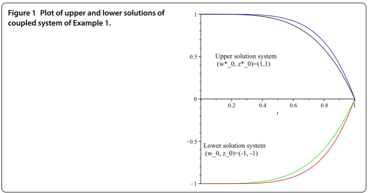
Example  Consider the following coupled system of coupled integral boundary values problem:

⎧ ⎪ ⎨ ⎪ ⎩

c_D__w₍_t_{) –}_w₍_t_{) +}_z₍_t_{) +  = ;} _t_∈_{(, ),} c_D_z₍_t_{) +}_w₍_t_{) –}_z₍_t_{) +  = ;} _t∈_{(, ),}

w() =z() = , w() =_tz(t)dt, z() =_tw(t)dt.

()

From the above system (), we see

t,w(t),z(t)= –w(t) +z(t) + , t,w(t),z(t)=w(t) –z(t) + . () Hereφ(t) =t,ϕ(t) =t. Alsoλ=λ=_,λ=_. Take (, ) = (w(),z()) and (, ) = (w,z) as

the initial approximation of the system of lower and upper solutions, respectively. Further, the function(t,w,z) is strictly decreasing with

–≤∂(t,w,z)

∂w = –w

_{< }

and(t,w,z) is strictly decreasing with

–≤∂(t,w,z)

∂z = –z

(12)

Figure 1 Plot of upper and lower solutions of coupled system of Example 1.

for all (w,z)∈[w(),z()]×[w,z]. Here the constantsc, dof the procedure are c= ,

d= . Thus (, ) and (, ) are the initial approximations of the lower and upper solutions, respectively, for the coupled system (). In Figure , we have ploted upper and lower solutions for the given system ().

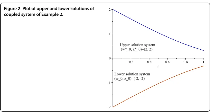
Example  For more explanation, we give another example of FDEs subject to the coupled

integral boundary conditions:

⎧ ⎪ ⎨ ⎪ ⎩

c_D__w₍_t_{) –}_w₍_t₎_exp₍_w₍_t_{)) +}_z₍_t_{) = ;} _t_∈_{(, ),} c_D__z₍_t_{) +}_w₍_t_{) –}_z₍_t₎_exp₍_z₍_t_{)) = ;} _t_∈_{(, ),}

w() =z() = , w() =_t_z₍_t₎_dt_, _z_{() =} t

_w₍_t₎_dt_.

()

From the above system (), we see

t,w(t),z(t)= –w(t)expw(t)+z(t), t,w(t),z(t)=w(t) –z(t)expz(t). ()

Here

φ(t) =t, ϕ(t) =t, also λ=λ=



, λ=

 .

Take (, ) = (w()_,_z()_{) and (, ) = (}_w

,z) as the initial approximation of the lower and

upper solutions, respectively. Then from (), we see that the function(t,w,z) is strictly decreasing with

–exp()≤∂(t,w,z)

∂w = –exp(w)(w+ ) < 

and(t,w,z) is strictly decreasing with

–exp()≤∂(t,w,z)

(13)

Figure 2 Plot of upper and lower solutions of coupled system of Example 2.

for all (w,z)∈[w()_,_z()_]_×_[_w

,z]. Here the constants c, dof the method are c=d=

exp(). Thus (, ) and (, ) are the initial approximations of the lower and upper solu-tions, respectively, for the coupled system (). Further, in Figure , we have ploted upper and lower solutions for the system ().

5 Conclusion

By the use of a monotone iterative technique, we successfully developed a scheme for or-der upper and lower solutions to the coupled system of highly nonlinear fractional oror-der diﬀerential equations with coupled integral boundary conditions. We have introduced an algorithm to construct a convergent increasing sequence of lower solutions as well as a convergent decreasing sequence of upper solutions. Further we have proved that the con-structed sequences converge uniformly to the unique solution of the considered problem. Moreover, the results are justiﬁed by some suitable numerical examples.

Acknowledgements

We are thankful to the anonymous referees for their useful comments, which completely modiﬁed and improved this paper. This work was supported by the National Natural Science Foundation of China (11571378).

Competing interests

It is declared that we have no conﬂict of interest.

Authors’ contributions

All authors equally contributed to this manuscript and approved the ﬁnal version.

Publisher’s Note

Springer Nature remains neutral with regard to jurisdictional claims in published maps and institutional aﬃliations.

Received: 14 March 2017 Accepted: 3 August 2017 References

1. Samko, GS, Kilbas, AA, Marichev, OI: Fractional Integrals and Derivatives: Theory and Applications. Gordon & Breach, Philadelphia (1993)

2. Podlubny, I: Fractional Diﬀerential Equations. Mathematics in Science and Engineering, vol. 198. Academic Press, New York (1999)

3. Hilfer, R: Applications of Fractional Calculus in Physics. World Scientiﬁc, Singapore (2000)

4. Pedersen, M, Lin, Z: Blow-up analysis for a system of heat equations coupled through a nonlinear boundary condition. Appl. Math. Lett.14(3), 171-176 (2011)

(14)

6. Khan, RA, Shah, K: Existence and uniqueness of solutions to fractional order multi-point boundary value problems. Commun. Appl. Anal.19, 515-526 (2015)

7. Benchohra, M, Graef, JR, Hamani, S: Existence results for boundary value problems with nonlinear fractional diﬀerential equations. Appl. Anal.87, 851-863 (2008)

8. Wang, J, Xiang, H, Liu, Z: Positive solution to nonzero boundary values problem for a coupled system of nonlinear fractional diﬀerential equations. Int. J. Diﬀer. Equ.2010, 1 (2010)

9. Yang, W: Positive solution to nonzero boundary values problem for a coupled system of nonlinear fractional diﬀerential equations. Comput. Math. Appl.63, 288-297 (2012)

10. Meehan, M, O’Regan, D: Multiple nonnegative solutions of nonlinear integral equations on compact and semi-inﬁnite intervals. Appl. Anal.74, 413-427 (2000)

11. Liu, X, Jia, M: Multiple solutions for fractional diﬀerential equations with nonlinear boundary conditions. Comput. Math. Appl.59, 2880-2886 (2010)

12. Nanware, JA, Dhaigude, DB: Existence and uniqueness of solution for fractional diﬀerential equation with integral boundary conditions. J. Nonlinear Sci. Appl.7, 246-254 (2014)

13. Leung, A: A semilinear reaction diﬀusion prey-predator system with nonlinear coupled boundary conditions: equilibrium and stability. Indiana Univ. Math. J.31, 223-241 (1982)

14. Kaur, A, Takhar, PS, Smith, DM, Mann, JE, Brashears, MM: Fractional diﬀerential equations based modeling of microbial survival and growth curves: model development and experimental validation. J. Food Sci.73(8), E403-E414 (2008) 15. Al-Refai, M: On the fractional derivatives at extreme points. Electron. J. Qual. Theory Diﬀer. Equ.2012, Article ID 55

(2012)

16. Wang, W, Agarwal, RP, Cabada, A: Existence results and the monotone iterative technique for systems of nonlinear fractional diﬀerential equations. Appl. Math. Lett.25(6), 1019-1024 (2012)

17. Lin, L, Liu, X, Fang, H: Method of upper and lower solutions for fractional diﬀerential equations. Electron. J. Qual. Theory Diﬀer. Equ.2012, Article ID 100 (2012)

18. McRae, FA: Monotone iterative technique and existence results for fractional diﬀerential equations. Nonlinear Anal., Theory Methods Appl.71, 6093-6096 (2009)

19. Shah, K, Khan, RA: Iterative scheme for a coupled system of fractional-order diﬀerential equations with three-point boundary conditions. Math. Methods Appl. Sci. (2016). doi:10.1002/mma.4122

20. Infante, G, Webb, JRL: Nonlinear nonlocal boundary value problems and perturbed Hammerstein integral equations. Proc. Edinb. Math. Soc.49, 637-656 (2006)

21. Ladde, GS, Lakshmikantham, V, Vatsala, AS: Monotone Iterative Techniques for Nonlinear Diﬀerential Equations. Pitman, Boston (1985)

22. Asif, NA, Khan, RA: Singular system with four point coupled boundary conditions. J. Math. Anal. Appl.386, 848-861 (2012)

23. Cui, Y, Zou, Y: Existence results and the monotone iterative technique for nonlinear fractional diﬀerential systems with coupled four-point boundary value problems. Abstr. Appl. Anal.2014, Article ID 242591 (2014)

24. Shah, K, Khalil, H, Khan, RA: Upper and lower solutions to a coupled system of nonlinear fractional diﬀerential equations. Prog. Fract. Diﬀer. Appl.2(1), 31-39 (2016)

25. Cui, Y, Zou, Y: Monotone method for diﬀerential system with coupled integral boundary value problems. Bound. Value Probl.2013, Article ID 245 (2013)

26. Cui, Y, Sun, J: On existence of positive solutions of coupled integral boundary value problems for a nonlinear singular superlinear diﬀerential system. Electron. J. Qual. Theory Diﬀer. Equ.2012, Article ID 41 (2012)

27. Miller, KS, Ross, B: An Introduction to the Fractional Calculus and Fractional Diﬀerential Equations. Wiley, New York (1993)

28. Wang, G: Monotone iterative technique for boundary value problems of a nonlinear fractional diﬀerential equation with deviating arguments. J. Comput. Appl. Math.236(9), 2425-2430 (2012)

29. Jia, M, Liu, X: Multiplicity of solutions for integral boundary value problems of fractional diﬀerential equations with upper and lower solutions. Appl. Math. Comput.232, 313-323 (2014)

30. Al-Refai, M: Basic results on nonlinear eigen value problems of fractional order. Electron. J. Qual. Theory Diﬀer. Equ.