Article
Vertex labeling and routing for Farey-type
symmetrically-structured graphs
Wenchao Jiang1, Yinhu Zhai2, Zhigang Zhuang1, Paul Martin3, Zhiming Zhao3and Jia-Bao Liu 4,*
1 School of Computer, Guangdong University of Technology, Guangzhou, 510006, China;
[email protected]; [email protected];
2 School of Information Engineering, Guangdong University of Technology, Guangzhou, 510006, China;
3 System and Network Engineering research group, Informatics Institute, University of Amsterdam, Science
Park 904, 1098XH, Amsterdam, the Netherlands; [email protected]; [email protected] 4 School of Mathematics and Physics, Anhui Jianzhu University, Hefei 230601, PR China;
* Correspondence: [email protected] Received: date; Accepted: date; Published: date
Abstract:The generalization of Farey graphs and extended Farey graphs are all originated from Farey graph and scale-free and small-world simultaneously. We propose a labeling of the vertices for it that allows determining all the shortest paths routing between any two vertices only based on their labels. The maximum number of shortest paths between any two vertices is huge as the product of two Fibonacci numbers, however, the label-based routing algorithm runs in linear timeO(n). The existence of an efficient routing protocol for Farey-type models should help the understanding of several physical dynamic processes on it.
Keywords: complex networks; deterministic models; Farey-type graphs; vertex labeling; shortest path routing;
1. Introduction
Deterministic models have unique advantages in improving our comprehension about some important physical mechanisms in complex networks. Especially, in comparison with the empirical and random graphs, the solutions of deterministic model can be obtained by rigorous derivation, and the computation can be ended only by a small amount of calculation. A lot of deterministic models are created imaginatively and studied carefully, which are inspired by simple recursive operation[1,2], or techniques of plane filling[3], or generating processes of fractal[4], or even the relationship between natural numbers[5]. Recently, on the basis of the classical Farey sequences, Zhang etc. introduced Farey graphs (FG) which are simultaneously minimally 3-colorable, uniquely Hamiltonian, maximally outer-planar and perfect[6,7]. The merger of three FG coincides with the network created by edge iterations[8], or evolving graphs with geographical attachment preference[9]; while the combination of six FG generates the graphs with multidimensional growth[10]. Moreover, two new kinds of Farey-type graphs, the generalization of Farey graphs (GFG) and the extended Farey graphs (EFG), are deduced by generalizing the construction mechanism of FG, and they all are scale-free and small-world[11–13].
Deterministic graphs also provide a new perspective and method on the classic research of physical processes. For example, some important dynamical processes on the basis of Apollonian models[14], a kind of deterministic graphs of scale-free, small-world, Euclidean, space-filling and matching graphs, are researched densely. The accurate analytical solutions are derived, including percolation[15], electrical conduction[14], Ising models[14], quantum transport[16], partially connected feedforward neural networks[17], traffic gridlock[18], Bose-Einstein condensation[19], Free-electron
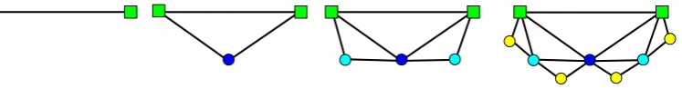
Figure 1.The Farey graphsF(t)at stepst=0, 1, 2, 3.
gas[20], and so on. However, the physical processes on FG are still lacking, for the recursive relationship in FG are more complex than Apollonian networks.
The routing protocol for the label-based all shortest paths may also bridge Farey-type graphs to the fields below. The all-pairs shortest paths problem is unquestionably one of the most well known problems in algorithm design, frequently studied in textbooks; yet, the complexity of the problem has remained open to this day. For arbitrary dense (directed and undirected) real-weighted graphs, the classical algorithms, such as Dijkstra, Bellman-Ford, A* and Floyd-Warshall, run in sub-cubic timeO(|V|3−δ), where
δ >0 [21–25].TheKshortest path routing (KSPR) algorithm is an extension algorithm of the shortest path routing algorithm in a given network[26], in whichKis the number of shortest paths to find. KSPR not only finds the shortest path, but alsoK−1 other paths in order of increasing cost. KSPR in Farey-type graphs will partly shrink to finding out all the shortest paths. The Graph Steiner tree problem (GSTR) is superficially similar to the minimum spanning tree problem: given a setVof vertices, interconnect them by a network of shortest length, where the length is the sum of the lengths of all edges[27]. GSTR has applications in circuit layout or network design, and most versions of GSTR are NP-complete. Moreover, for the bottleneck of many network analysis algorithms is the extortionate computational complexity of calculating the shortest paths, scientists have only to study the approximate algorithm of it[28].
Graphs are composed of vertices and edges and are very often studied considering branch of discrete mathematics known as graph theory. One active subject in graph theory is graph labeling. This is not only due to its theoretical importance but also because of the wide range of applications in many fields, such as crystallography, coding theory, circuit design and communication design[29]. Finding shortest paths in graphs is a well-studied and important problem with also many applications. On the relationship between vertices labels and the shortest paths, several deterministic models have been pioneered by Zhang and Camellas [29–32]. Only by their labels, one of shortest paths is determined just by simple rules and few computations.
Here we provide a labeling method for Farey-type graphs, so that queries for all the shortest paths between any pair of vertices can be efficiently answered thanks to it. In spite of the huge number of shortest paths between two vertices, the routing algorithm runs in linear timeO(n).
2. Generation of Farey-type graphs
For GFG and EFG are generalized from FG, we present the definitions of the three in turn. Definition 2.1(Generation of FG) Farey graphF(t) = (V(t),E(t)), in which the iteration step 0≤t, with vertex setV(t)and edge setE(t)is constructed as follows[6]:
• Fort=0,F(0)has two initial vertices and an edge joining them.
• Fort≥1,F(t)is obtained fromF(t−1)by adding to every edge introduced at stept−1 a new vertex adjacent to the end vertices of this edge (see Fig.1).
RemarkThe order and size of FG are|V(t)| =2t+1 and|E(t)| =2t+1+1, respectively. The number of vertices adding at steptisnt=2t−1. The cumulative degree distribution ofF(t)follows an exponential distributionPcum(δ) =2−δ2, and the degree correlationskm(δ)is approximately a linear function ofδ, which suggests that FG is assortative [6, 7].
( 1)
F t
1 2
X X X
1
Y
1( )
y V t
1 ( )
xy V t
1( )
x V t
1( )
F t
2
Y
2( )
x V t
2 ( )
xy V t
2( )
y
V t F t2( )
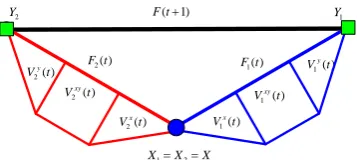
Figure 2.Schematic illustration of construction ofF(t+1).
Figure 3.The generalization of Farey graphsGF(t,k)at stepst=0, 1and2 whenk=2.
Vx(t)(includingX) have shorter distances from them to Xthan to Y, while the vertices in Vy(t) (includingY) have shorter distances toYthan to X. If the distances are equal, vertices are all in
Vxy(t).That is to say,V(t) =Vx(t)∪Vxy(t)∪Vy(t). Noticing that, the distances differences above are 0 or 1, forXandYare neighbors. From Fig.2, if two copies ofF(t)are named asF1(t)andF2(t), with
initial verticesX1,Y1andX2,Y2, thenF(t+1)is generated just by merging initial verticesX1andX2
intoXand linkingY1andY2intoYdirectly, and the hub ofF(t+1)isXobviously.
Definition 2.2(Generation of GFG)GF(t,k)is deduced by the rules:
• Fort=0,GF(0)is composed of three initial vertices which are linking each other.
• Fort≥1,GF(t)is constructed fromGF(t−1,k)by addingknew vertices adjacent to the two end vertices of every edge introduced at stept−1, then linking theknew vertices to the two end vertices (see Fig.3).
Remark GF(t, 1)is exactly the graphs created by edge iterations[8], or evolving graphs with geographical attachment preference[9]. GFG can also be treated as a flower which has 3×ksame pedals, which are noting asPi(t),i = 1, 2, . . . , 3×k. All pedals rooted from two initial vertices, for GFG is made up of three groups, so that each group containsksame pedals.
Definition 2.3(Generation of EFG) The construction ofEF(t,k)is shown as below:
• Fort=0,EF(0,k)holds three vertices which are linking each other.
• Fort≥1,EF(t,k)originates fromEF(t−1,k)by addingknew vertices to every edge introduced at stept−1 and three edges added at t = 0, then linking theknew vertices to the two end vertices (see Fig.4).
Figure 4.The extended Farey graphsEF(t,k)at stepst=0, 1,and2 whenk=2.
5.1
5.2
5.3
5.4 4.1
4.2 3.1 0.0
5.5 5.6 5.7 5.8
4.3 4.4
3.2 2.1
5.9 5.10 5.11 5.12 4.5
4.6 3.3 1.1 5.13
5.14 5.15 5.16
4.7 4.8
3.4
2.2 0.1
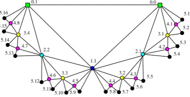
Figure 5.Labels of all vertices inF(t)whent=5.
3. Labeling and routing ofF(t)
The labeling and routing protocol of GFG and EFG are extended from FG, here we firstly proposal the algorithms of it for completeness.
Definition 3.1The labeling of any vertex in FG is performed according to the following rules:
• Label two initial vertices as 0.0 and 0.1.
• At stept ≥1, the adding new vertices are marked with labels fromt.1 tot.2t−1in clockwise direction (see Fig.5).
Supposing any two vertices are labeled withti.kandtj.landti≥tj, then the mother vertex ofti.kjoins in graph at stepti−1, while the father vertex adds to graphs at stepti−2 or earlier. Two vertices with same mother are brothers. The relationships between different vertices, as the following properties, are extracted by the help of their labels.
Property 3.1 (The family of ti.k )
Whenti ≥1, two children oftj.kare(ti+1).2kand(ti+1).(2k−1). Whenti ≥2, the brother ofti.(k+1)forkis odd, orti.(k−1)forkis even. When ti ≥ 2, ti.k and its parents shape a triangle, the mother is (ti−1).
j K
2
k
, the father is
(ti−l).
jk−rem(k,2)
2t
k
, in whichbxc= f loor(x)is a function rounding the real numberxtoward negative infinity,rem(k, 2)is the remainder ofkdivided by 2, the integerl(≥2)denotes the sum of one and the number of the continuous zeros from right to left in the binary sequence which is converted by the decimal numberk−rem(k, 2).
Ifti≥tj, the(ti−tj)thgeneration of maternal ancestor ofti.kistj. j
k
2ti−tj
k .
Proof Several results are very obvious besides the father’s label, here we only proof it. Ifti≥2 andt= ti−tj, thus,t∈ {2, . . . ,ti−2}. Whenkis even,tis the sum of one and the number of the continuous zeros from right to left of the binary numbers ofk, so that the father’s label ist−∆t.j2k∆t
right to left of the binary numbers ofk−1, the father labels witht−∆t.jk2−1∆t
k
. Whenk=1, the father ofti.lis 0.0 for anyti. In summary, whenti ≥2, the father ofti.kis marked with(ti−l).
jk−rem(k,2)
2l
k .
Property 3.2 (The neighbors ofti,k) Whenti ≥2, he neighbors ofti.kis{(ti−l).
jk−rem(k,2)
2l
k
,(ti−1). j
k
2
k
,(ti+x).2x−1(2k−1),(ti+
x).
2x−1(2k−1) +1
}, x∈ {1, 2, . . . ,t−ti}.
When ti = 1, the neighbors of 1.1 are {0.0, 0.1,(1 + x).2x−1(2k − 1),(1 +
x).
2x−1(2k−1) +1
}, ti ∈ {0, 1, 2, . . . ,t}.
Whenti=0, the neighbors of 0.0 and 0.1 are{ti.1}, ti∈ {0, 1, 2, . . . ,t}and{0.0,ti.2ti−1}, ti ∈
{1, 2, . . . ,t}.
Proof This property can be proved obviously, for the neighbors ofti.kare all family members by property 3.1.
Property 3.3 When two vertices are located in different sub-graphsF1(t−1)andF2(t−1)ofF(t), the hubXofF(t)is on the shortest paths, if
a)ti.k∈V1x(t−1)∪V
xy
1 (t−1)andtj.l∈V2x(t−1)∪V
xy
2 (t−1),
b) orti.k∈V2x(t−1)∪V
xy
2 (t−1)andtj.l∈V1x(t−1)∪V
xy
1 (t−1),
c) orti.k∈V1x(t−1)andtj.l ∈V y
2(t−1)/{Y2},
d) orti.k∈V2x(t−1)andtj.l∈V1y(t−1)/{Y1}.
Two initial verticesY1andY2ofF(t)are located on the shortest paths, if
a)ti.k∈V1y(t−1)andtj.l∈V2y(t−1),
b) orti.k∈V y
2(t−1)andtj.l∈V y
1(t−1).
VerticesX,Y1andY2lie on the shortest paths simultaneously, if
a)ti.k∈V1y(t−1)andtj.l∈V2xy(t−1),
b) orti.k∈V2y(t−1)andtj.l∈V1xy(t−1).
Proof F(t)is combined with two sub-graphsF1(t−1)andF2(t−1). Same asF(t), all the vertices
inFη(t−1) (η=1, 2)can be divided into three groupsVηx(t−1),V
xy
η (t−1)andV
y
η(t−1)similarly. Ifti.k∈V1x(t−1)∪V
xy
1 (t−1)andtj.l∈V2x(t−1)∪V
xy
2 (t−1), the routes betweenti.kandtj.lshould go byX, or byY1andY2;but the distance byXis shorter than byY1andY2so that the shortest paths in
this condition passX.The proof of the other seven conditions is similar.
Property 3.4All the shortest paths between any pair of vertices are located in a minimum common sub-graph (MCSG) denoting asFncsg(tmin), moreover, one vertex is positioned in the outermost layer ofFηmcsg(tmin−1), the other is an initial vertex or a(p+1)thlayer vertex inF
mcsg
3−η (tmin−1).
Proof By the construction algorithm of F(t), all the shortest paths between ti.k and tj.l are irrelevant to vertices which are adding toF(t)after step ti. That is to say, all the shortest paths are located in an embedded sub-graphF(ti). However, the relationship of their positions may be more closely, the minimum embedded sub-graph, orFmcsg(tmin), is obtained by decreasingtitill the minimumtmin.
Case 1: Ifl=j k 2ti−tj
k
Ifti.kis a neighbor oftj.l, by property 3.2, MCSG isF(0).
Ifk= (l−1)×2ti−tj+2ti−tj−1+2, ork∈ {(l−1)×2ti−tj−1+3,(l−1)×2ti−tj+2ti−tj−1+4},
or . . ., ork ∈ {(l−1)×2ti−tj +2ti−tj−1+2ti−tj−2+1,l×2ti−tj}, MCSG isF(2), or F(3), or . . ., or F(ti−tj), respectively. In these conditions,tj.lis the initial vertex 0.0 of MCSG.
Ifk ∈ {(l−1)×2ti−tj+2ti−tj−1−2}, ork ∈ {(l−1)×2ti−tj +2ti−tj−1−3,(l−1)×2ti−tj +
2ti−tj−1−4}, or . . ., ork∈ {(l−2)×2ti−tj+1,(l−1)×2ti−tj+2ti−tj−1}, MCSG isF(2), orF(3), or
. . ., orF(ti−tj).and Vertextj.lis the other initial vertex 0.1 inFmcsg(tmin). Case 2: Ifl6=m=j k
2ti−tj
k
By 2p−1≤ |m−l| ≤2p,Fmcsg(t
min) =F(ti−tj+p+1), thenti.kis an outermost layer vertex in
Fηmcsg(tmin−1)andtj.lis a(p+1)thlayer vertex inF
mcsg
The detailed shortest routing protocol betweenti.kandtj.lis shown as follows. Firstly, find out
Fmcsg(tmin)forti.kandtj.l. Then, determine the hubXand two initial verticesY1andY2ofFmcsg(tmin) are whether on the shortest paths or not. Thirdly, form new pairs of vertices from vertices ofti.k,tj.l,x,
Y1andY2, then go to the first step. Repeat three steps till all pairs of vertices are neighbors. Property 3.5 (The shortest paths routing algorithm of Farey graphs)
1. Given a pair of vertices is labeled withti.kandtj.l. 2. Determine whether the two vertices are neighbors or not.
Ifti−tj=1 andl= j
k
2
k
, orti−tj=mandl =
jk−rem(k,2)
2m
k
, by property 3.1, two vertices are mother-child or father-child relationship. Insert the two labels to the labels set of the shortest paths (LSSPm(h)). Noticing thatLSSPm(0) =∅andmis an integer increasing from one. Go to step 6th.
3. Find out MCSG whenl=j k 2ti−tj
k
, namely,tj.lis the(ti−tj)thgeneration of maternal ancestor ofti.k.
Ifk∈ {(l−1)×2ti−tj +2ti−tj−1+2}, ork∈ {(l−1)×2ti−tj+2ti−tj−1+2,(l−1)×2ti−tj−1+
4}, or . . ., ork∈ {(l−1)×2ti−tj +2ti−tj−1+2ti−tj−2+1,l×2ti−tj}, MCSG is the embedded
sub-graph fromF(2)toF(ti−tj).tj.lis the initial vertex 0.0 andti.kis an outermost layer vertex in MCSG.
Ifk ∈ {(l−1)×2ti−tj +2ti−tj−1−2}, ork ∈ {(l−1)×2ti−tj +2ti−tj−1−3,(l−1)×2ti−tj +
2ti−tj−1−4}, or . . ., or k ∈ {(l−1)×2ti−tj +1,(l−1)×2ti−tj +2ti−tj−1} , MCSG is also
sub-graphs fromF(2)toF(ti−tj), buttj.lis the other initial vertex 0.1. Go to step 5th. 4. Find out MCSG whenjl6=m= k
2ti−tj
k .
Fortj.mis the(ti−tj)thgeneration of maternal ancestor ofti.k, thenFmcsg(tmin) = F(ti−tj+
p+1), in which 2p−1≤ km−lk ≤2p. Go to step 5th.
5. DetermineX,Y1andY2of MCSG are whether on the shortest paths or not.
Map the labels ofFmcsg(tmin)into labels ofF(tmin), divide all the vertices inF(tmin)into six sets as above:Vηx(tmin−1),Vηxy(tmin−1)andV
y
η(tmin−1). Then, decideX,Y1andY2are whether on the shortest paths by property 3.3 or not.
IfXis on the paths, insert the label ofX, assumingtp.q, in the middle ofti.kandtj.linLSSPm(h), andh=h+1. Therefore, go to step 1st with two new pairs of labels:ti.kandtp.q,tp.qandtj.l. IfY1andY2in it, insert the labels ofY1andY2,tp1.qlandtp2.q2, in the middle ofti.kandtj.lin
LSSPm(h), andh=h+2. Get two new pairs of labels,ti.kandtp1.ql,tp2.q2 andtj.l. Go to step 1st.
IfX,Y1andY2are all on the paths at same time, inserttp.qintoLSSPm(h)andh=h+1, then inserttp1.q1 andtp2.q2 intoLSSPm+1(h),h=h+2. Go to step 1st with four pairs of labels:ti.k andtp.q,tp.qandtj.l,ti.kandtp1.q1,tp1.q1,tp2.q2 andtj.l.
6. Ascertain the shortest paths routing.
The shortest paths are traversed every elements in every set ofLSSPm(h)in order, wheremis the number of the shortest paths andhis the distance betweenti.kandtj.l.
The time complexity of the shortest paths routing algorithm is related to the maximum number of the shortest paths between any two vertices in Farey graphs. The number is exactly the product of two Fibonacci numbers (Fn, in whichFn = Fn−1+Fn−2andF0 = F1 = 1 ) in FG.
From the construction mechanism, all the vertices on the shortest paths shape rhombuses which are zigzagged adjacent, so that the maximum number of rhombuses from ti.k to 0.
j k
2ti−2
k
is jti 2
k
and from tj.l to 0. j
l
2tj−2
k
is jtj−32 k. Therefore, the number of shortest paths from
ti.kto 0. j
k
2ti−2
k isFj
ti
2 k
+1 = 1 √ 5
(1+ √
t
2 )
j
ti
2+l
k
−(1− √
5 2 )
j
ti
2 k
+1
1 0 2 2.1.1.2 2.1.1.1 0.1.1.2 1.1.1.2 1.1.1.1 0.1.1.1 0.2.1.1 0.2.1.2 0.2.1.3 0.2.1.4 0.2.2.1 0.2.2.2 0.2.2.3 0.2.2.4 1.2.1.1 1.2.1.2 1.2.1.3 1.2.1.4 1.2.2.1 1.2.2.2 1.2.2.3 1.2.2.4 2.2.1.4 2.2.1.3 2.2.1.2 2.2.1.1 2.2.2.1 2.2.2.2 2.2.2.3 2.2.2.4
(a)GF(2, 2).
1 0 2 2.1.1.2 2.1.1.1 0.1.1.2 1.1.1.2 1.1.1.1 0.1.1.1 0.2.1.1 0.2.1.2 0.2.1.3 0.2.1.4 0.2.2.1 0.2.2.2 0.2.2.3 0.2.2.4 1.2.1.1 1.2.1.2 1.2.1.3 1.2.1.4 1.2.2.1 1.2.2.2 1.2.2.3 1.2.2.4 2.2.1.4 2.2.1.3 2.2.1.2 2.2.1.1 2.2.2.1 2.2.2.2 2.2.2.3 2.2.2.4 0.1.1.3 0.1.1.4 2.1.1.3 2.1.1.4 1.1.1.3 1.1.1.4
(b)EF(2, 2).
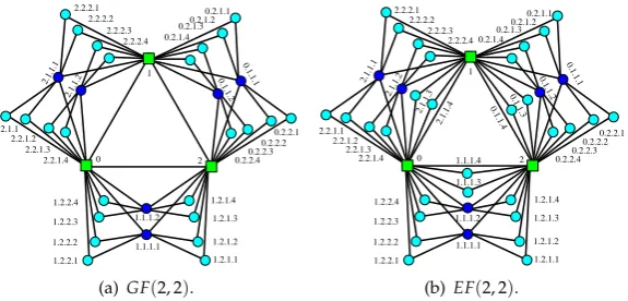
Figure 6.The labeling ofGF(t,k)andEF(t,k)at step t=2 for k=2.
0.j l
2tj−2
k isF
tj−3 2
+1=
1 √ 5
(1+
√ 5 2 )
tj−3 2
+1
−(1− √
5 2 )
tj−3 2
+1
, so that the maximum number
is Fj
ti
2 k
+1×Ftj−3
2
+1 = 1 5[(1+
√ 5 2 ) j ti 2 k +1
−(1− √ 5 2 ) j ti 2 k +1 ]
(1+
√ 5 2 )
tj−3 2
+1
−(1− √
5 2 )
tj−3 2
+1
.
Whenti = tj = t, the number in FG is Fbt
2c+1×Fbt−23c+1 =
1 5[(1+
√ 5 2 )b
t
2c+1−(1−
√ 5 2 )b
t
2c+1]
[(1+ √
5 2 )b
t−3
2 c+1−(1−
√ 5 2 )b
t−3
2 c+1], and it increases almost exponentially. Fortunately, only at most 2t+1 vertices are needed to be ascertaining in the routing algorithm, and only several operations of additions and multiplications are needed for determining one vertex whether on the shortest paths or not. As a result, all the shortest paths between any pair of vertices can be determined in linear time ofO(n).
Property 3.6The shortest paths routing algorithm between any two vertices of Farey graphs runs in linear time.
4. Labeling ofGF(t,k)andEF(t,k)
Definition 4.1(The labeling of GFG) The labeling of any vertex inGF(t,k)shows as the following rules:
• The three initial vertices are labeled with 0, 1 and 2.
• At any stept ≥ 1, a vertex inGF(t,k)is marked with a.b.c.d according to thegroup(a), the
subgroup(b.c)and the precisepositions(d)from down to top in the same subgroup, in which
a∈ {0, 1, 2}, b={1, 2, . . . ,t} c=∈ {1, 2, . . . , 2b−1}andd∈ {1, 2, . . . ,kb}. Definition 4.2 (The labeling of EFG) Vertices inEF(t,k)are labeled as follows:
• Label three initial vertices as 0, 1 and 2.
• At stept ≥ 1, a vertex is tagged witha.b.c.d, in whicha ∈ {0, 1, 2}, b ∈ {1, 2, . . . ,t}, c ∈ {1, 2, . . . , 2b−1}andd∈ {1, 2, . . . ,(t−b+1)×kb}.
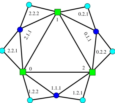
Labeling ofGF(2, 2)andEF(2, 2)are illustrated in Fig.6.
Remark For GFG have more pedals than EFG, so thatdmax = (t−b+1)×kbin EFG, while
dmax =kbin GFG.
Whent≥2, any new vertex, adding to GFG/EFG at stepti, links to two vertices: a mother and a father. The vertices adding to graphs at the same time are multiple births if they have the same parents. Supposing that two arbitrary vertices in GFG/EFG are labeled witha1.b1.c1.d1anda2.b2.c2.d2,
0.1 .1
0
1
2 2.1
.1
1.1.1 2.2.2
2.2.1
0.2.1
0.2.2
1.2.1 1.2.2
Figure 7.The projected graph ofGF(2, 2)/EF(2.2).
Property 4.1 (The family of a.b.c.d) Whenb ≥ 1, a.b.c.d belongs to a set of multiple births
{a.b.c.(kjdkk+1),a.b.c.(kjdkk+2), . . . ,a.b.c.(kjdkk+k)}.
Whenb≥2,a.b.c.dand its parents shape a triangle, the mother isa.(b−1).c
2
.jdkk, the father is
a.(b−1).jc−rem(c2l ,2)
k .jkdl
k .
Ifb≥b0, the(b−b0)thgeneration of maternal ancestor ofa.b.c.disa.b0.
j c
2b−b0 k
.j d kb−b0
k .
Proof Several results are very obvious besides the father’s label, here we only proof it. Ifb≥2, letldenotes the differenceb−b1, thus,l∈ {2, . . . ,b−2}. Whencis even, the time differencelis the sum of one and the number of the continuous zeros from right to left of the binary numbers ofc, so that the father’s label isa.(b−l).j2cl
k .jkdl
k
; Whencis odd but excluding one,lis the sum of one and the number of the continuous zeros from right to left of the binary numbers ofc−1, the father labels witha.(b−l).jc2−ll
k .jkdl
k
; Whenc=1 and with anyb, the fathers are all the initial vertex. In summary, the father ofa.b.c.disa.(b−l).jc−rem(c2l ,2)
k .jkdl
k
whenb≥2.
RemarkThe vertexa.1.1.dhas two mothers{0, 1, 2}/{a}and no father. Three initial vertices have no parents and multiple births. Therefore, the neighbors ofa.b.c.dare derived by property 4.2.
Property 4.2(The neighbors ofa.b.c.d)
When b ≥ 2, the set of neighbors of a.b.c.d is {a.(b − l).jc−rem(c2l ,2)
k .jkdl
k
, a.(b −
1)c
2
.jdkk, a.(b+x).2x−1(ac−1).d, a.(b+x).[2x−1(2c−1) +1].d}, in whichx∈ {1, 2, . . . ,t−b}
,d∈ {(b+x−1)×kx+1,(b+x−1)×kx+2. . . . ,(b+x)×kx}.
The neighbors of initial vertexaare{0, 1, 2}/{a} ∪ {a.b.1.d} ∪ {a.b.2b−1.d}, whereb∈ {1, 2, . . . ,t},
d∈ {1, 2, . . . ,kb}.
The neighbors ofa.1.1.dare{0, 1, 2}/{a}and{a.(1+x).2x−1.d, a.(1+x).(2x−1+1).d}, where
x∈ {1, 2, . . . ,t−1},d∈ {(b+x−1)×kx+1,(b+x−1)×kx+2, . . . ,(b+x)×kx}.
Property 4.3 (The projection of GFG/EFG) By merging verticesa.b.c.d, which have samea.b.cbut differentd, into a vertex labeling witha.b.c,GF(t.k)/EF(t,k)is projected into a graph which is exactly the combination of three Farey graphs starting from every edge of a triangle.
Proof From the spatial relationship between vertices in different pedals, all the vertices ofa.1.1.d
are linked to common vertices till two initial vertices{0, 1, 2}/{a}, so that all ofa.1.1.dcan merged into a vertex ofa.1.1.By recursively using the spatial relationship,GF(t,k)/EF(t,k)is projected into a combination of three Farey graphs.
Property 4.4 (The slice shapes bya.b.c.d) For any vertexa.b.c.d, the slice is obtained by recursively finding out all triangles which are shaped by a vertex and its parents, till two initial vertices.
Proof Any vertexa.b.c.dhas a fathera.(b−l).jc−rem(c2l ,2)
k .jkdl
k
and a mothera.(b−1).c
2
.jdkk y property 4.1, and the three vertices shaped a triangle. Then, the father’s mother, or the mother’s father, is got by recursively using property 4.1. From the spatial relationship of vertices,a.b.c.dand all these parents shape a slice.
5. Routing ofGF(t,k)andEF(t,k)
Although the labels of three initial vertices are slightly different from labels of two initial vertices in FG, the shortest paths protocol in GFG/EFG also benefit from the routing algorithm in FG. From the generation mechanism, GFG/EFG is divided into three groups by symmetry, and each group is consisted ofkort×kpedals, furthermore, vertices in each group can also be divided into three sets by the distance differences, similar to that of FG:Vx(t),Vxy(t)andVy(t).
Property 5.1 (The characteristic of shortest paths when two vertices are located in different groups)
Ifa1 6= a2, the initial vertex{0, 1, 2}/{a1,a2}is on the shortest roads betweena1.b1.c1.d1and
a2.b2.c2.d2of GFG/EFG, if a)a1.b1.c1∈V1x(t)∪V
xy
1 (t)anda2.b2.c2∈V2x(t)∪V
xy
2 (t),
b) ora1.b1.c1∈V2x(t)∪V
xy
2 (t)anda2.b2.c2∈V1x(t)∪V
xy
1 (t),
c) ora1.b1.c1∈V1x(t)anda2.b2.c2∈V2y(t)/{a2}, d) ora1.b1.c1∈V2x(t)anda2.b2.c2∈V1y(t)/{a1}.
The two initial verticesa1anda2are on the shortest ways, if
a)a1.b1.c1∈V1y(t)anda2.b2.c2∈V2y(t),
b) ora1.b1.c1∈V2y(t)anda2.b2.c2∈V1y(t).
The shortest paths pass{0, 1, 2}/{a1,a2},a1anda2simultaneously, if a)a1.b1.c1∈V1y(t)anda2.b2.c2∈V
xy
2 (t),
b) ora1.b1.c1∈V2y(t)anda2.b2.c2∈V1xy(t).
Proof From the property 4.3,a1.b1.c1.d1anda2.b2.c2.d2are projected asa1.b1.c1anda2.b2.c2, which are located in different sub-graphsF1(t)andF2(t)of Farey graphsF(t+1). imilar as the proof of property 3.3, the conclusions can easily be deduced.
Property 5.2 (The characteristic of shortest paths when two vertices lie in different slices of same group) Ifa.b1.c1.d1anda.b2.c2.d2are located in different pedals, the shortest paths between them are positioned in two slices which are connected by two common vertices of them.
Proof From the generating algorithm, ifa.b1.c1.d1anda.b2.c2.d2are located in different pedals or
sub-pedals, the neighbor sets ofa.b1.c1.d1anda.b2.c2.d2are ascertained by property 4.2. When two common neighbors are getting at the same step, thena.b1.c1.d1anda.b2.c2.d2are positioned in different slices, and the two slices can be determined by property 4.4. Supposing that the first two common neighbors area.b3.c3.d3anda.(b3+1).c4.d4, the two slices root from it and belong toF(b1−b3)and F(b2−b3). Compared with the construction schematic diagram in Fig.2, the linking ofF(b1−b3)and
F(b2−b3)has slightly difference. Named the initial vertices ofF(b1−b3)andF(b2−b3)asX1,X2and
Y1,Y2, respectively.F(b1−b3)andF(b2−b3)is linked exactly by mergingX1andY1intoa.b3.c3.d3and
linkingX2andY2intoa.(b3+1).c4.d4.The vertices ofF(b1−b3)andF(b2−b3)can be divided into
six parts similarly:Vαx(t),Vαxy(t),V
y
α(t)andVβx(t),V
xy
β (t),V
y
β(t), by the distance betweena.b1.c1.d1 ora.b2.c2.d2to initial verticesX(i.e. a.b3.c3.d3) andY(i.e. a.(b3+1).c4.d4), then the shortest paths betweena.b1.c1.d1anda.b2.c2.d2go bya.b3.c3.d3, if
a)a.b1.c1∈Vαx(t)anda.b2.c2∈V
x
β(t), b)a.b1.c1∈Vαx(t)anda.b2.c2∈V
xy
β (t), b) ora.b1.c1∈Vαxy(t)anda.b2.c2∈Vβx(t).
The shortest paths go througha.b3.c3.d3anda.(b3+1).c4.d4, if
a)a.b1.c1∈Vαx(t)anda.b2.c2∈V
b) ora.b1.c1∈Vαxy(t)anda.b2.c2∈V
xy
β (t), c)a.b1.c1∈Vαy(t)anda.b2.c2∈Vβx(t). The shortest paths passa.(b3+1).c4.d4, if a)a.b1.c1∈Vαxy(t)anda.b2.c2∈Vβy(t),
b)a.b1.c1∈Vαy(t)anda.b2.c2∈V
xy
β (t), b) ora.b1.c1∈Vαy(t)anda.b2.c2∈V
y
β(t).
Property 5.3 (The characteristic of shortest paths when two vertices are in same slice) Ifa.b1.c1.d1
anda.b2.c2.d2are in the same slice of a pedal or sub-pedal of same group, the shortest paths between
them are determined by property 3.5, for they have been projected into a Farey graph.
Proof If we obtained only one common neighbor vertex, labeling with a.b3.c3.d3, of vertices
a.b1.c1.d1anda.b2.c2.d2at the same step, thena.b1.c1.danda.b2.c2.d2are located in same slice. Assuming
b1≥b2, the projected Farey graph isF(b1−b3−1)with huba.b1.c1.d1, then, all the shortest paths are
located inF(b1−b3−1). So that all the shortest paths can be decided by property 3.5. Then, the detailed shortest routing algorithm in GFG/EFG is described as follows.
Property 5.4 (The shortest paths routing algorithm in GFG/EFG)
• Given any two vertices area1.b1.c1.d1anda2.b2.c2.d2. Inserta1.b1.c1.d1anda2.b2.c2.d2to the labels
set of the shortest paths (LSSPm(h)),LSSPm(0) =∅.
• Ifa16=a2and,a1.b1.c1.d1anda2.b2.c2.d2are not initial vertex. This is exactly the condition of
two vertices in different groups. Three initial vertices{0.1.2}/{a1,a2},a1anda2are ascertained on the shortest paths or not by property 5.1.
If{0, 1, 2}/{a1,a2}is on the roads, insert the label{0, 1, 2}/{a1,a2}in the middle ofa1.b1.c1.d1
anda2.b2.c2.d2inLSSPm(h),h = h+1, and generate two new pairs of labels: a1.b1.c1.d1and
{0, 1, 2}/{a1,a2},{0, 1, 2}/{a1,a2}anda2.b2.c2.d2, respectively.
If a1 anda2 are on it, insert the labels a1 anda2 in the middle of two labels a1.b1.c1.d1 and
a2.b2.c2.d2,h=h+2, and get two new pairs of labels:a1.b1.c1.d1anda1,a2anda2.b2.c2.d2.
If{0, 1, 2}/{a1,a2},a1anda2are all on it, combine the two conditions above together.
Go to step 1st.
• Ifa16=a2, anda1.b1.c1.d1ora2.b2.c2.d2is an initial vertex. It is the case of two vertices locating in
a same slice of a pedal or sub-pedal in same group. The common Farey graphsF(b1)orF(b2)is obtained by property 5.3, then, the shortest paths are deduced by property 3.5.
• Ifa1=a2=aanda.b1.c1.d1anda.b2.c2.d2are not initial vertices, find out neighbors ofa.b1.c1.d1
anda.b2.c2.d2by property 4.2.
If two common neighbors are obtained at the same step, thena.b1.c1.d1anda.b2.c2.d2are located
in different slices. Whether the two common neighbors are positioned on the shortest paths or not are determined by property 4.6. Assuming two common neighbors area.b3.c3.d3anda.b4.c4.d4, ifa.b3.c3.d3(ora.b4.c4.d4) is on the shortest paths, insert the labela.b3.c3.d3(ora.b4.c4.d4) in the middle ofa1.b1.c1.d1anda2.b2.c2.d2,h =h+1, and generate two new pair labels ofa1.b1.c1.d1
anda.b3.c3.d3(ora.b4.c4.d4), anda.b3.c3.d3(ora.b4.c4.d4) ora2.b2.c2.d2. Ifa.b3.c3.d3anda.b4.c4.d4
are on the shortest paths at the same time, insert the labela.b3.c3.d3anda.b4.c4.d4in the set
LSSPm(h),h=h+1,m=m+1, and make up four new pair labels ofa1.b1.c1.d1anda.b3.c3.d3,
a1.b1.c1.d1anda.b4.c4.d4,a.b3.c3.d3ora2.b2.c2.d2,a.b4.c4.d4anda2.b2.c2.d2. Go to step 1st.
If only a common neighbor is obtained at the same time, thena.b1.c1.d1anda.b2.c2.d2are located in same slice. The shortest paths are projected into a Farey graph, and then all the shortest paths are derived by Property 3.5.
withd ≥ 1 andt ≥ 0, are constructed as follows. Fort = 0, A(d, 0)is a complete graphKd+2(or d+1-clique).Fort ≥ 1, A(d,t)is obtained from A(d,t−1). For each of the existing subgraphs of
A(d,t−1)that is isomorphic toa(d+1)-clique and created at stept−1, a new vertex is created and connected to all the vertices of this subgraph. Apparently,A(1,t)is exactly the same as the special case of the generalization of Farey graphsGF(t, 1), however, the algorithm in[31] can only get one of shortest paths in it.
The recursive clique-trees, which have small-world and scale-free properties and allow a fine tuning of the clustering and the power-law exponent of their discrete degree distribution[32]. The recursive clique-treeK(q,t)(q≥1,t≥0)is the graph constructed as follows: Fort=0,K(q, 0)is the complete graphKq (or q-clique).ForK(q,t)is obtained from byK(q,t−1)(i) adding for each of its existing subgraphs isomorphic to a q-clique a new vertex and (ii) joining it to all the vertices of this subgraph. From the construction mechanisms,K(2,t)is the same as the extended Farey graphs of
EF(t, 1).
6. Conclusion
We presented label-based routing algorithm for Farey-type graphs, including Farey graphs, the generalization of Farey graphs and the extended Farey graphs. Our results can be extended easily to several Farey-type deterministic models, such as the model created by edge iterations, evolving graphs with geographical attachment preference, general geometric growth model for pseudofractal scale-free web, the graphs with multidimensional growth and so on. Different from the former research results, they can only get one shortest path from the labels of any pair vertices; we can ascertain all the shortest paths only by their labels in all Farey-type graphs.
For all Farey-type graphs are structure isomorphic, the time complexities of the routing algorithm in the generalization of Farey graphs and the extended Farey graphs are essentially equivalent to which on Farey graphs, thus, the routing algorithms runs in linear timeO(n).
Our solutions can also be easily extended to several weighted or delayed models, such as weighted scale-free small-world graphs[33] and delayed pseudofractal graphs[34].
Author Contributions:Wenchao Jiang contribute for conceptualization, designing the experiments, analyzed the data curation and wrote the paper. Yinhua Zhai and Zhigang Zhuang contribute for performed experiments, resources, software, some computations. Paul Martin, Zhiming Zhao and Jia-Bao Liu contribute for supervision, methodology, validation and formalanalysing. All authors read and approved the final version of the paper.
Funding:This work was supported by the National Science Foundation of China under grant No.11601006; the Natural Science Foundation of Guangdong Province [grant no.2016A030313703]; the Guangdong Science and Technology Plan [grant no.2016B030305002, 2017B010124001 and 2017B090901005]; the European Union’s Horizon 2020 research and innovation program [grant No.654182 (ENVRIPLUS project)] and [grant No.676247 (VRE4EIC project)]; the China Postdoctoral Science Foundation under grant No. 2017M621579 and Postdoctoral Science Foundation of Jiangsu Province under grant No.1701081B.
Conflicts of Interest: The authors declare no conflict of interest.
1. Comellas, F., Ozon, J., & Peters, J. G. (2000). Deterministic small-world communication networks. Information Processing Letters, 76(1), 83-90.
2. Barabási, A. L., Ravasz, E., & Vicsek, T. (2001). Deterministic scale-free networks. Physica A: Statistical Mechanics and its Applications, 299(3), 559-564.
3. Andrade Jr, J. S., Herrmann, H. J., Andrade, R. F., & Da Silva, L. R. (2005). Apollonian networks: Simultaneously scale-free, small world, Euclidean, space filling, and with matching graphs. Physical Review Letters, 94(1), 018702.
4. Zhang, Z., Gao, S., Chen, L., Zhou, S., Zhang, H., & Guan, J. (2010). Mapping Koch curves into scale-free small-world networks. Journal of Physics A: Mathematical and Theoretical, 43(39), 395101.
6. Zhang, Z., & Comellas, F. (2011). Farey graphs as models for complex networks. Theoretical Computer Science, 412(8), 865-875.
7. Zhang, Z., Wu, B., & Lin, Y. (2012). Counting spanning trees in a small-world Farey graph. Physica A: Statistical Mechanics and its Applications, 391(11), 3342-3349.
8. Zhang, Z., Rong, L., & Guo, C. (2006). A deterministic small-world network created by edge iterations. Physica A: Statistical Mechanics and its Applications, 363(2), 567-572.
9. Zhang, Z. Z., Rong, L. L., & Comellas, F. (2006). Evolving small-world networks with geographical attachment preference. Journal of Physics A: Mathematical and General, 39(13), 3253.
10. Peng, A., & Zhang, L. (2011). Deterministic multidimensional growth model for small-world networks. arXiv preprint arXiv:1108.5450.
11. Zhang, Z., Rong, L., & Zhou, S. (2007). A general geometric growth model for pseudofractal scale-free web. Physica A: Statistical Mechanics and its Applications, 377(1), 329-339.
12. Havlin, S., & ben-Avraham, D. (2007). Fractal and transfractal recursive scale-free nets. New Journal of Physics, 9(6), 175.
13. Xiao, Y., & Zhao, H. (2013, July). Counting the number of spanning trees of generalization Farey graph. In Natural Computation (ICNC), 2013 Ninth International Conference on (pp. 1778-1782). IEEE.
14. Andrade Jr, J. S., Herrmann, H. J., Andrade, R. F., & Da Silva, L. R. (2005). Apollonian networks: Simultaneously scale-free, small world, Euclidean, space filling, and with matching graphs. Physical Review Letters, 94(1), 018702.
15. Auto, D. M., Moreira, A. A., Herrmann, H. J., & Andrade Jr, J. S. (2008). Finite-size effects for percolation on Apollonian networks. Physical Review E, 78(6), 066112.
16. Almeida, G. M., & Souza, A. M. (2013). Quantum transport with coupled cavities on an Apollonian network. Physical Review A, 87(3), 033804.
17. Wong, W. K., Guo, Z. X., & Leung, S. Y. S. (2010). Partially connected feedforward neural networks on Apollonian networks. Physica A: Statistical Mechanics and its Applications, 389(22), 5298-5307.
18. Mendes, G. A., Da Silva, L. R., & Herrmann, H. J. (2012). Traffic gridlock on complex networks. Physica A: Statistical Mechanics and its Applications, 391(1), 362-370.
19. de Oliveira, I. N., de Moura, F. A. B. F., Lyra, M. L., Andrade Jr, J. S., & Albuquerque, E. L. (2010). Bose-Einstein condensation in the Apollonian complex network. Physical Review E, 81(3), 030104.
20. De Oliveira, I. N., De Moura, F. A. B. F., Lyra, M. L., Andrade Jr, J. S., & Albuquerque, E. L. (2009). Free-electron gas in the Apollonian network: Multifractal energy spectrum and its thermodynamic fingerprints. Physical Review E, 79(1), 016104.
21. Knuth, D. E. (1977). A generalization of Dijkstra’s algorithm. Information Processing Letters, 6(1), 1-5. 22. Yen, J. Y. (1970). An algorithm for finding shortest routes from all source nodes to a given destination in
general networks. Quarterly of Applied Mathematics, 27(4), 526.
23. Delling, D., Sanders, P., Schultes, D., & Wagner, D. (2009). Engineering route planning algorithms. In Algorithmics of large and complex networks (pp. 117-139). Springer Berlin Heidelberg.
24. Zwick, U. (2002). All pairs shortest paths using bridging sets and rectangular matrix multiplication. Journal of the ACM (JACM), 49(3), 289-317.
25. Chan, T. M. (2010). More algorithms for all-pairs shortest paths in weighted graphs. SIAM Journal on Computing, 39(5), 2075-2089.
26. Yen, J. Y. (1971). Finding the k shortest loopless paths in a network. management Science, 17(11), 712-716. 27. Bern, M. W., & Graham, R. L. (1989). The shortest-network problem. Scientific American, 260(1), 84-89. 28. Zwick, U. (2001). Exact and approximate distances in graphs—a survey. In Algorithms—ESA 2001 (pp. 33-48).
Springer Berlin Heidelberg.
29. Zhang, Z., Comellas, F., Fertin, G., Raspaud, A., Rong, L., & Zhou, S. (2008). Vertex labeling and routing in expanded Apollonian networks. Journal of Physics A: Mathematical and Theoretical, 41(3), 035004. 30. Comellas, F., & Miralles, A. (2009). Vertex labeling and routing in self-similar outerplanar unclustered graphs
modeling complex networks. Journal of Physics A: Mathematical and Theoretical, 42(42), 425001.
31. Comellas, F., & Miralles, A. (2011). Label-based routing for a family of scale-free, modular, planar and unclustered graphs. Journal of Physics A: Mathematical and Theoretical, 44(20), 205102.
33. Zhang, Y., Zhang, Z., Zhou, S., & Guan, J. (2010). Deterministic weighted scale-free small-world networks. Physica A: Statistical Mechanics and its Applications, 389(16), 3316-3324.