102 | P a g e
EXPONENTIAL B-SPLINE COLLOCATION METHOD
FOR THE NUMERICAL SOLUTION OF ONE-SPACE
DIMENSIONAL NONLINEAR WAVE EQUATION
WITH STRONG STABILITY PRESERVING TIME
INTEGRATION
Rajni Arora
1, Suruchi Singh
2, Swarn Singh
3 1Department of Mathematics, University of Delhi, New Delhi (India)
2
Department of Mathematics, Aditi Mahavidyalaya, University of Delhi, (India)
3
Department of Mathematics, Sri Venkateswara College, University of Delhi, New Delhi (India)
ABSTRACT
In this paper, a new numerical method is presented to approximate the solution of second order one-dimensional nonlinear wave equation. The method is based on collocation of exponential B-splines. Exponential B-splines are applied for spatial variable and derivatives. The method produces two systems of first order ordinary differential equations. We solve these systems using strong stability preserving methods. Numerical experiments are presented to illustrate the accuracy and efficiency of the proposed method.
Keywords:
Exponential B-Spline Method, SSP-HBT54 Method, SSP-RK54 Method, Tri-Diagonal
Solver, Wave Equation
I. INTRODUCTION
We consider the following one-space dimensional nonlinear hyperbolic partial differential equation:
subject to the initial conditions:
and the boundary conditions:
The numerical solution of second order one space dimensional nonlinear wave equation is of great importance
in various fields of sciences. Many researchers have studied various numerical techniques for the solution of
linear and non-linear wave equations. Gao, Chi [1] presented unconditionally stable schemes for one
dimensional linear hyperbolic equation. Mohanty et al [2]-[6] proposed several methods based on uniform and
103 | P a g e
polynomial slpines have been developed for the solution of equation (1). Recently, Mittal and Bhatia [7]
presented modified cubic B-spline Differential Quadrature Method for the solution of (1). Not much work based
on exponential splines has been done. However, it is being stated by McCartin [8], [9] that the exponential
splines are more general splines. McCartin further stated that cubic splines many times exhibit unwanted
oscillations in the form of overshoots and/or extraneous inflection points and that exponential splines can
remedy this situation for appropriately chosen tension parameters. Reza Mohammadi used exponential B-spline
for solving Convection-Diffusion equations in [10]. We, in this paper, present the collocation method based on
exponential B-spline basis functions to solve some benchmark nonlinear wave equations. Equation (1) is
converted into a system of partial differential equations and then exponential B-spline collocation method is
used to discretize the equations spatially which leads to formulation of two systems of first order ordinary
differential equations which are then solved by SSP-RK54 [11] and SSP-HBT54 [12] methods respectively.
The outline of the paper is as follows: In section 2, we discuss exponential B-spline collocation method. In
section 3, we apply this method to nonlinear hyperbolic wave equations. Numerical experiments are illustrated
in section 4 and finally concluding remarks are given in section 5.
II. EXPONENTIAL B-SPLINE COLLOCATION METHOD
In exponential B-splines collocation method the approximate solution can be written as a linear combination of
exponential B-spline basis functions for the approximation space under consideration. We consider a mesh
as a uniform partition of the solution domain by knots with
spacing for
The exponential B-splines at the above defined knots together with additional knots are given
by:
where
where is a free parameter. Additional knots are required to define all the exponential splines. The
104 | P a g e
function is twice continuously differentiable. The values of at knots are tabulated in
Table 1.
Table 1: Values of exponential B-spline and its derivatives at different knots
0 1 0
0 0 0
0 0
In the collocation method with exponential B-splines, an approximate solution to the analytical
solution can be written in the form:
where are unknown quantities to be determined from the boundary conditions and collocation form of the
differential equation (1). In order to eliminate the coefficients and , we redefine the exponential
B-spline basis functions as:
Then, the approximate solution can be rewritten as the linear combination of redefined exponential
B-spline basis functions (6) as:
From equation (7) and Table 1, the approximate values of and its first and second order derivatives
are determined in terms of the time parameters as follows:
where
III. NUMERICAL METHOD
105 | P a g e
Then using (7), the approximate values of and can be written as:
where is the derivative of with respect to and is the derivative of with respect to .
Evaluation at the boundary knots:Imposing boundary conditions and using the redefined basis functions (6)
and Table 1 in (10), we can write system (9) at the boundary knots as:
and
Evaluation at the internal knots:Using the redefined basis functions (6) and Table 1 in (10) and (11), we can
write system (9) at the interior knots as
Finally, using the definition of basis functions (6) and Table 1, equation (14) can be written as the following
systems of ordinary differential equations:
which in matrix form can be written as:
where, , , , , ,
where,
and denotes for .
To compute the solution at the required knots, the vector is to be determined at each time level. We solve
106 | P a g e
evaluated from (16) by using tri-diagonal solver. Then the obtained system of equations along with the system
(17) gives first order ordinary differential equations. We solve the former system for by SSP-RK54 method
and the latter for by SSP-HBT54 method. Consequently, on using (8), the approximate solution is
obtained.
To initiate the computation we need initial vectors, and which can be determined by using initial
conditions (2):
, , which in matrix form can be written as:
where,
, , and , .
Now, is a tri diagonal matrix, hence, equation (18) can be solved for by tri-diagonal solver.
Similarly, second initial condition gives
, ,
i.e. we have,
Hence, from (19), initial vector can be calculated.
IV. NUMERICAL EXPERIMENTS
In this section, we present the numerical results of present method on one linear and four nonlinear wave
equations. We also compare obtained results with the results obtained by existing methods. For all the problems
we choose . The accuracy of the presented method is measured using errors, maximum absolute errors
(MAE) and root mean square errors (RMSE).
,
MAE ,
RMSE .
where and denote the exact and approximate solutions respectively.
Example 1. (Wave equation in polar coordinates)
This equation represents one-dimensional wave equation in cylindrical and spherical coordinates for and
2 respectively. The analytical solution is . The initial and boundary conditions can be
107 | P a g e
proposed method are given in Table 2 for . A comparison between analytical and numerical solution
upto for is done by plotting space time graphs which are given in Fig. 1 and Fig. 2. It is clear from
the Table and graphs that our method is efficient in approximating the solution of wave equation in polar
coordinates.
Table 2: MAE error for example 1 at t=2 with
MAE CPU time(in sec) MAE CPU time(in sec)
0.25 4.3651e-04 1.13 4.7525e-04 1.13
0.50 5.3182e-04 2.19 6.3619e-04 2.17
0.75 6.0372e-04 3.22 9.5102e-04 3.23
1 5.3498e-04 4.31 9.9524e-04 4.24
Figure 1: Analytical solution of example 1 for
108 | P a g e
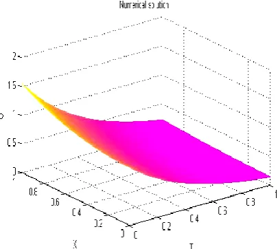
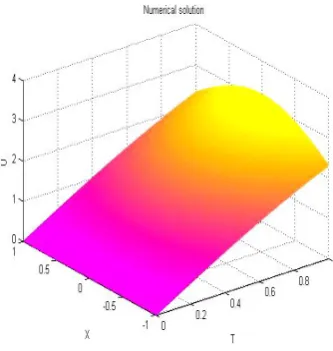
Example 2. (Van der Pol type nonlinear wave equation)
The analytical solution is The maximum absolute errors obtained at for
and different values of are given in Table 3. A comparison between analytical solution and
numerical solution upto for , and can be done by studying Fig. 3 and Fig. 4.
It is evident from the figures that our method is efficient in approximating solution of Van der pol type nonlinear
wave equation.
Table 3: MAE error for example 2 at
with
.3.6000e-03 1.7000e-03 7.2618e-04
9.2084e-04 4.3797e-04 1.8142e-04
2.3184e-04 9.7609e-05 4.4266e-05
5.8628e-05 2.7616e-05 9.9387e-06
109 | P a g e
Figure 4: Numerical Solution of Example 2 for
, ,
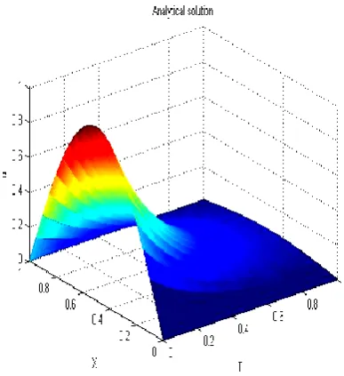
Example 3. (Dissipative non-linear wave equation)
.
The analytical solution is . The maximum absolute errors and root mean square errors
at different times and , are tabulated in Table 4. The results obtained are compared with
the results obtained by Mittal and Bhatia [7]. Our results are in good agreement with the results obtained in [7].
Space-time graphs of analytical and numerical solutions are given in Fig. 5 and Fig. 6 respectively, which also
confirm the accuracy of the method.
Table 4: Errors for Example 3 for =0.05,
Our Method Mittal and Bhatia [7]
RMSE MAE RMSE MAE
1 2.0000e-03 2.8000e-03 3.046e-03 4.274e-03
2 1.9000e-03 2.6000e-03 3.251e-03 4.625e-03
3 2.8396e-05 3.8175e-05 5.737e-05 9.782e-05
110 | P a g e
Figure 6: Numerical solution of example 3 upto for
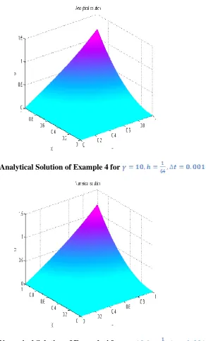
Example 4. (Non-linear wave equation)
The analytical solution is . We report the maximum absolute errors obtained at for
in Table 5. The calculations are carried out for different values of and . Space-time graphs of
analytical and numerical solution are also plotted in Fig. 7 and Fig. 8.
Table 5: MAE for Example 4 at =1 with
=0.001
7.1000e-03 1.3400e-02 3.5400e-02
1.9000e-03 3.7000e-03 9.8000e-03
6.6791e-04 1.2000e-03 3.3000e-03
111 | P a g e
Figure 7: Analytical Solution of Example 4 for
Figure 8: Numerical Solution of Example 4 for
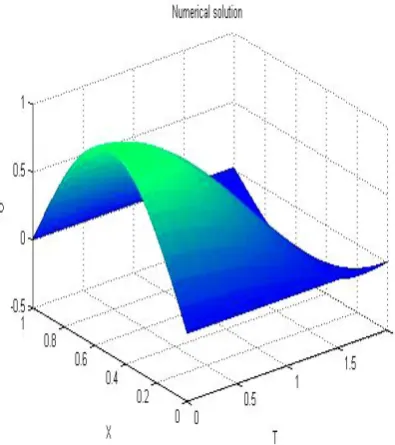
Example 5. Consider the following Sine-Gordan equation:
The analytical solution is . This example is solved at different time levels for
. The results obtained are compared with the results obtained by Dehghan and
Shokri [13]. It is evident from the Table 6 that our results are in good agreement with the results obtained by
Dehghan and Shokri [13]. Moreover, the numerical solution obtained for is compared
with the analytical solution in Fig. 9 and 10.
112 | P a g e
Table 6: Errors Calculated for Example 5 for
Proposed Method Dehghan and Shokri [13]
MAE MAE MAE
.25 3.0413e-06 1.0875e-05 1.0875e-05 5.3761e-06 3.91e-05 5.89e-06
.50 1.2125e-05 4.5317e-05 4.5317e-05 1.4216e-05 1.30e-04 2.01e-05
.75 2.7560e-05 1.0236e-04 1.0236e-04 3.5439e-05 2.35e-04 3.63e-05
1 5.4593e-05 2.0372e-04 2.0372e-04 6.0377e-05 3.27e-04 5.07e-05
Figure 9: Analytical Solution of Example 5 for
Figure 10: Numerical Solution of Example 5 for
V. CONCLUSION
In this paper, an exponential B-spline collocation method has been proposed to solve second order one
dimensional nonlinear wave equation. The second order problem is first converted into two first order partial
differential equations. Then, exponential B-spline collocation method is applied to convert these equations into
113 | P a g e
five stage, fourth order Runge-Kutta method and Hermite-Birkhoff-Taylor method respectively. This choice of
methods gives better results compared to the results obtained by using one of them only. The main advantage of
this method is that because of its simplicity, it is easy to be applied to any linear or nonlinear problem available
in literature and gives accurate results.
REFERENCES
[1] F. Gao and C. Chi, Unconditionally stable difference schemes for a one-space-dimensional linear
hyperbolic equation, Applied Mathematics and computation, 187, 2007, 1272-1276.
[2] R.K. Mohanty and S. Singh, High order variable mesh approximation for the solution of 1D non-linear
hyperbolic equation, International Journal of Nonlinear Science, 14(2), 2012, 220-227.
[3] R.K. Mohanty and S. Singh, High accuracy Numerov type discretization for the solution of one-space
dimensional non-linear wave equations with variable coefficients, Journal of Advanced Research in Scientific Computing, 3, 2011, 53-66.
[4] R.K. Mohanty, M.K. Jain and K. George, On the use of high order difference methods for the system of
one space second order nonlinear hyperbolic equations with variable coefficients, Journal of Computational and Applied Mathematics, 72(2), 1996, 421-431.
[5] R.K. Mohanty, M.K. Jain and S. Singh, A new three-level implicit cubic spline method for the solution of
1D quasi-linear hyperbolic equations, Computational Mathematics and Modeling, 24(3), 2013, 452-470. [6] R.K. Mohanty and V. Gopal, A fourth order finite difference method based on spline in tension
approximation for the solution of one-space dimensional second-order quasi-linear hyperbolic equations,
Advances in Difference Equations, 70(1), 2013, 1-20.
[7] R.C. Mittal and R. Bhatia, Numerical solution of some nonlinear wave equations using modified cubic
B-spline Differential quadrature method, 2014 International Conference on Advances in Computing, Communications and Informatics, 2014, 433-439.
[8] B.J. McCartin, Theory of exponential splines, Journal of Approximation Theory, 66, 1991, 1-23.
[9] B.J. McCartin, Computation of exponential splines, SIAM Journal on Scientific and Statistical Computing, 2, 1990, 242-262.
[10] R. Mohammadi, Exponential B-spline solution of Convection-Diffusion equations, Applied Mathematics, 4, 2013, 933-944.
[11] R. Spiteri and S. Ruuth, A new class of optimal high-order strong-stability-preserving time discretization
methods, SIAM Journal on Numerical Analysis, 40, 2002, 469-491.
[12] T. Nguyen-Ba, H. Nguyen-Thu and T. Giordano, One-step strong-stability-preserving
Hermite-Birkhoff-Taylor methods, Scientific Journal of Riga Technical University, 45, 2010, 95-104.
[13] M. Dehghan and A. Shokri, A numerical method for one-dimensional nonlinear Sine-Gordan equation,
Numerical methods for Partial Differential equations, 24(2), 2008, 687-698.