Surface Rust Detection Using Ultrasonic Waves in a Cylindrical Geometry by Finite Element Simulation

(1)

Surface Rust Detection Using Ultrasonic Waves in a

Cylindrical Geometry by Finite Element Simulation

Qixiang Tang1, Cong Du2, Jie Hu1, Xingwei Wang2and Tzuyang Yu1,*

1 _{Department of Civil and Environmental Engineering, One University Avenue, Lowell, MA 01854, U.S.A.} 2 _{Department of Electric and Computer Engineering, One University Avenue, Lowell, MA 01854, U.S.A.}

* Correspondence: [email protected]; Tel.: +1-978-934-2288

Version July 10, 2018 submitted to Preprints

Abstract: Detection of early stage corrosion on slender steel members is crucial for preventing 1

buckling failures of steel structures. An active photoacoustic fiber optic sensors (FOS) system 2

has been reported for early stage steel corrosion detection of steel plates and rebars using surface 3

ultrasonic waves. The objective of this paper is to investigate the surface corrosion/rust detection 4

problem on steel rods using numerically simulated surface ultrasonic waves. The finite element 5

method (FEM) is applied in simulating the propagation of ultrasonic waves on steel rod models. 6

Transmission mode of damage detection is adopted, in which one source (transmitter) and one sensor 7

(receiver) are considered. In this research, radial displacements at the receiver were simulated and 8

analyzed by short-time Fourier transform (STFT) for detecting, locating, and quantifying a surface 9

rust located between the transmitter and the receiver. From our time domain and frequency domain 10

analyses, it is found that the presence, location, and dimensions (length, width, and depth) of surface 11

rust can be estimated by ultrasonic waves propagating through the surface rust. 12

Keywords: finite element method (FEM); damage detection; surface rust; ultrasonic testing; 13

short-time Fourier transform 14

1. Introduction 15

Slender steel members such as steel rods and bars are widely used structural components in 16

civil infrastructure (e.g., steel truss bridges, temporary support structures, traffic signs). Unlike 17

other construction materials such as Portland cement concrete, steel is vulnerable to corrosion. Steel 18

corrosion can take place when suitable environmental conditions (e.g., temperature, pH, oxygen, 19

moisture, chloride ions) are met. As a result, premature failures of steel structures can occur if one or 20

many critical members is corroded. Corrosion of steel members will reduce the effective cross sectional 21

area of the member by replacing steel (ferrite) with rust (ferrite oxides). Consequently, structural 22

stiffness and bearing capacity of corroded steel members will be reduced. Furthermore, corrosion of 23

steel members can also increase the likelihood of instability (buckling) for slender steel members, due 24

to the change of boundary condition at the support or within each member. 25

Detection of early stage corrosion on slender steel members is crucial for preventing their 26

premature failures. Various nondestructive evaluation/testing (NDE/T) and structural health 27

monitoring (SHM) techniques have been applied to steel structures [1]. Example techniques include 28

visual testing [2], modal analysis [3], Eddy current testing [4], thermal infrared testing [5], and 29

ultrasonic testing [6,7]. Among these techniques, fiber optic sensors (FOS) represent a popular approach 30

for long-term monitoring of steel structures [8,9]. While FOS have been applied to many steel structures 31

in the past, most of the damage detection algorithms are based on passive response of FOS. In other 32

words, either corrosion-induced cracking or loading-induced dynamic response must be generated 33

from monitored steel members such that FOS can passively detect the presence of corrosion. Recently, 34

an active photoacoustic FOS system has been reported for early stage steel corrosion detection of steel 35

plates and rebars [10]. Different from traditional passive FOS techniques, active FOS can generate 36

acoustic/ultrasonic waves to probe monitored steel members for early-stage corrosion detection. 37

(2)

2 of 18

Meanwhile, installed FOS allow engineers to assess the conditions (e.g., temperature) of structures 38

without the use of couplant and "adapters" [11–13]. With a minimized size, active FOS can be installed 39

onto irregular/curved surface of structures. 40

In this paper, our objective is to investigate the surface rust detection problem in a cylindrical 41

geometry (slender steel rod) using ultrasonic waves in transmission mode and to develop a surface 42

rust detection algorithm., as a basis for the practical application of an active photoacoustic FOS system. 43

Steel rods are chosen as an example of slender steel members. The finite element method (FEM) is 44

applied in simulating the propagation of ultrasonic waves at 1MHz on steel rod models. Surface rust is 45

simulated by a rectangular prism which is characterized by its location (s3), length (d), width (w), and 46

depth (h). Transmission mode of damage detection is adopted, in which one source (transmitter) and 47

one sensor (receiver) are considered. In this research, radial displacements (u(t)) at the receiver were 48

simulated and analyzed by short-time Fourier transform (STFT) for detecting, locating, and quantifying 49

a surface rust located between the transmitter and the receiver. Time domain and frequency domain 50

analyses are conducted for developing a damage detection algorithm. In what follows, the detail of 51

finite element (FE) simulation is first provided. 52

2. Finite element simulation 53

In the past, FEM had been applied for simulating ultrasonic wave propagation for damage 54

detection [14–16]. Among various signal processing techniques, short-time Fourier transform (STFT) 55

has been demonstrated as an applicable approach for analyzing the transient response of ultrasonic 56

wave propagation in the time-frequency domain [17]. In this research, cylindrical geometry was 57

numerically modeled by six steel rod models (one intact and five corroded) in a commercially 58

available finite element package (ABAQUS 2016) [18]. 705, 600 linear hexahedral elements (C3D8) 59

were used in all six models. Five corroded steel rod models were created by introducing a rectangular 60

prism/anomaly to the surface of intact steel rod model. Transmission mode of damage detection was 61

applied for data collection by using one transmitter (source orT) and one receiver (R) in each model, 62

as shown in Fig.1. Time domain radial displacement (u(t)) at the receiver was collected for all six 63

models. Design of intact and corroded FE models are described in the following sections. 64

2.1. Intact steel rod model 65

An intact steel rod model (denoted by IM) was created by using a cylinder with 12.7-mm diameter 66

(D) and 50-mm length, as shown in Fig.1. Materials properties of steel used in the intact steel rod 67

model was provided in Table1. A transmitter (T) was located at mid-span and a receiver (R) was 68

located 10 mm away fromTalong the longitudinal axis (z-axis) of the model. The distance betweenT 69

andRwas denoted ass1. The intact steel rod model was fixed at both ends. To suppress unnecessary 70

reflections from both ends, ten absorbing layers [19] were used at each end of the model such that 71

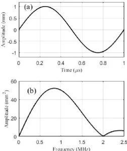
ultrasonic waves propagating into the absorbing layers can be damped out. As shown in Fig.2), a 72

sinusoidal pulse was introduced atT, and time domain radial displacement (u(t)) was collected atR. 73

Table 1.Material’s properties

Material Density (kg/m3) Young’s Modulus (MPa) Poisson’s Ratio

Steel 7,850 210,000 0.3

Rust 2,610 500 0.3

2.2. Corroded steel rod models 74

Five corroded steel rod models (denoted by CM) were generated by replacing the material 75

properties at a corroded region from steel to rust in order to simulate the introduction of surface rust to 76

the intact steel rod model, as shown in Table2. Four attributes were used to characterize the corroded 77

Preprints (www.preprints.org) | NOT PEER-REVIEWED | Posted: 10 July 2018 doi:10.20944/preprints201807.0170.v1

(3)

Figure 1.Intact steel rod model

region (surface rust): location (s3), length (d), width (w) and thickness (h). Two values were considered 78

for each attribute. 79

Table 2.Five corroded steel rod models

Model Surface rust location s3(mm)

Surface rust length d(mm)

Surface rust width w(mm)

Surface rust thickness h(mm)

CM1 4 2 2.2 1

CM2 6 2 2.2 1

CM3 4 4 2.2 1

CM4 4 2 4.4 1

CM5 4 2 2.2 0.5

3. Research hypotheses and approach 80

3.1. Hypotheses of ultrasonic waves propagation in intact and corroded rod models 81

Five hypotheses on ultrasonic waves propagation in intact and corroded steel rod models were 82

made for the damage detection problem in this paper. A Mercator projection of cylindrical geometry 83

for steel rod models is provided in Fig.3to better illustrate these hypotheses. 84

1. In model IM, time domain radial displacementu(t)is collected atR. The first ultrasonic wave 85

packet is the one propagating along the~s1path at a velocity ofc1and arriving at timet1. The 86

second ultrasonic wave packet propagates along the~s2path and arriving at timet2with a velocity 87

ofc2. 88

2. In corroded steel rod models (CM1 CM5), the ultrasonic waves propagating along the~s1path 89

(4)

4 of 18

Figure 2.Designed loading function

waves propagates through the surface rust and arrives at timet0₁(i.e.,t0₁>t1since the ultrasonic 91

wave velocity in rust is slower than the one in steel). 92

3. Part of the ultrasonic waves is scattered from the surface rust and propagates along the~s4path. 93

Timet0₂ is the total time of flight (TOF) of scattered ultrasonic wave propagating along path 94

(~s3,~s4)(t02=t3+t4). Propagation velocities of ultrasonic waves on path~s1and path(~s3,~s4)are 95

respectivelyc0₁andc0₂. 96

4. In Fig.3(top view), path~s8is the path of ultrasonic waves diffracted by the surface rust (~s8 = 97

~s6+d+~s7). TOF of these ultrasonic waves ist8(i.e.,t8=t6+td+t7). 98

5. Higher frequencies are affected more than lower frequencies by the presence of surface rust. 99

This is because that the effective depth of each frequency is approximately its wavelength [20]. 100

With ’shallow’ effective depth, higher frequencies interact with the surface rust more than lower 101

frequencies. 102

3.2. Damage detection algorithm 103

Based on the aforementioned five hypotheses, surface rust detection, localization and 104

quantification are carried by the following approach. 105

3.2.1. Damage detection 106

In this paper, detection of surface rust can be accomplished by determining the reduction of 107

centroid frequency (∆fc) in the spectrogram of u(t)by using STFT. The steps of obtaining fcare

108

reported in the following. 109

1. Generate/introduce ultrasonic waves at transmitterTof model IM. 110

(5)

Figure 3.Mercator projection of intact and corroded surface for ultrasonic wave propagation paths

2. Collect time domain radial displacementu(t)at receiverR. 111

3. Apply short-time Fourier transform (STFT) to u(t)in order to convert it to its spectrogram 112

U(t,f). 113

4. In the spectrogramU(t,f), show the half-power contour at -3 dB from the maximum amplitude 114

of the first wave packet. 115

5. Determine the centroid of the half-power contour for the first wave packet by finding its 116

coordinates(fc,tc)in the spectrogramU(t,f).

117

6. The centroid frequency fcof this FE simulation is found. For intact model (IM), fc= fc,i.

118

7. Repeat the steps for an artificially corroded model. For corroded models, fc= fc,c.

119

Fig.4illustrates the parameters defined in the steps for damage detection, using model CM1 as an 120

example. Eq. (1) shows the damage detection criterion for detecting the presence of surface rust. 121

∆fc= fc,i−fc,c

(

=0 intact

6

=0 corroded (1)

where∆fc= difference in the centroid frequency between intact and corroded steel rod models (in

122

MHz), fc,i= centroid frequency of model IM (in MHz), and fc,c= centroid frequency of corroded steel

123

rod models (in MHz). In this research, a steel rod model is considered intact (no damage) if there is no 124

reduction of centroid frequency or∆fc=0 and vice versa.

125

3.2.2. Damage localization 126

To locate surface rust, TOF (time-of-flight) of scattered ultrasonic waves is used. In this research, 127

the location of surface rust is defined by the length of path~s3ors3=|~s3|. The value ofs3indicates the 128

location of surface rust. 129

TOF of the scattered wave (t0₂) traveling through path~s3and~s4is defined by 130

(6)

6 of 18

Figure 4.Procedure of obtainingfcvalue

where t3 and t4 = TOF of ultrasonic waves propagating on paths~s3 and~s4 (µs)), respectively. 131

Equivalently, 132

t0₂(s3,s4) =

s3

c1

+s4 c4

(3)

wheres3= length of path~s3(mm),s4(s3)= length of path~s4(mm) = p

(s1−s3)2+p2,p= perimeter 133

of the rod model (mm),c1= propagation velocity on path~s1(mm/µs), andc4= propagation velocity 134

on path~s4(mm/µs). From our previous study, a propagation velocity model (Eq. (4)) based on the 135

length of path on a cylindrical geometry was reportedc4[17]. 136

c4(s4) =a+b

p s4

(4)

whereaandb= model parameters. By substituting Eq. (4) and re-arranging terms, we have 137

h

(s1−s3)2+p2 i

c1− t02−s3a q

(s1−s3)2+p2−t02c1bp+s3bp=0 (5) wheres1= length of path~s1(mm). In Eq. (5),s1,p, andc1must be provided. Parametersaandb 138

are from reported literature [17]. Timet0₂is measured from a corroded model. Once timet0₂is measured, 139

Eq. (5) can be solved by the graphic method. Eq. (5) also represents the damage localization criterion 140

in our algorithm. Finding the value ofs3locates the surface rust in this research. 141

(7)

3.2.3. Damage quantification 142

For damage quantification, dimensions of surface rust (lengthd, widthw, and thicknessh) are to 143

be found. In finding the lengthdof surface rust, TOF (t0₁) of ultrasonic waves propagating through 144

surface rust and arriving at receiverRis used. Timet0₁denotes the total propagation time along path 145

~s1which consists of path~s3, surface rust (lengthd), and path~s5. In other words, 146

t0₁=t3+t5+tr (6)

wheret0₁= total TOF of ultrasonic wave propagating on path~s1(µs), t3= TOF of ultrasonic wave 147

traveling on path~s3(µs), t5 = TOF of ultrasonic wave traveling on path~s5(µs)), andtr = TOF of

148

ultrasonic wave traveling within surface rust (µs). Sinces1=s3+d+s5, we have 149

t0₁(d) = s1−d c1

+ d

cr (7)

wherecr= propagation velocity on z-axis in rust (mm/µs). By re-arranging Eq. (7), surface rust length 150

dcan be directly determined by 151

d(t0₁) = crs1−crc1t 0

1

cr−c1

(8)

Eq. (7) represents thelength estimationcriterion in our algorithm. 152

Onces3(from damage localization, Eq. (5)) andd(from Eq. (8)) are determined, the width of 153

surface rust (w) can be obtained by using the delayed arrival time of first wave packet (t8), as shown in 154

Fig.3(top view). Eq. (9) describes the relationship betweent8andw. 155

t8c1− q

s2

3+ (w/2)2−d− q

s2

5+ (w/2)2=0 (9)

wheres5=s1−d−s3,t8= TOF of ultrasonic wave propagating on path~s8and 156

~s8=~s6+d+~s7 (10)

in a corroded steel rod model (µs),s6= length of path~s6(mm) ands7= length of path~s7(mm). Eq. (9) 157

represents thewidth estimationcriterion in our algorithm. 158

From our fifth hypothesis (Section 3.1), lower frequency ultrasonic waves have ’deeper’ effective 159

depths. It suggests that more frequencies in the STFT spectrogram will be affected when increasing the 160

thicknesshof surface rust. This phenomenon is illustrated by the reduction of spectrograms’ curvature 161

or ∂ 2_U

1

∂f2 and modeled by an empirical equation as shown in Eq. (11). 162

h

∂2U1

∂f2

=e∂

2_U 1

∂f2 +g (11)

whereh = thickness of surface rust (mm), ∂2U1

∂f2 = second-order partial derivative of the first wave 163

packet’s frequency domain projection, and eand g = model parameters. ∂2U1

∂f2 approximates the

164

curvature of the first wave packet. Eq. (11) represents the thickness estimationcriterion in our 165

algorithm. 166

Eqs. (8), (9) and (11) represent our damage quantification approach in this paper. Surface rust 167

lengthd, widthw, and thicknesshcan be estimated from the STFT spectrogram of radial displacement 168

(8)

8 of 18

4. Simulation results and findings 170

Time domain radial displacement (u(t)) of each model at receiverRwas collected from six FE 171

simulation cases (one for intact model and five for corroded models). Spectrogram (U(f,t)) of each 172

u(t)was obtained by STFT. Comparison ofu(t)andU(f,t)between intact and corroded steel rod 173

models was made to study the effects of surface rust onu(t)andU(f,t). 174

4.1. Time domain response 175

In each model, radial displacementu(t)are receiver Rwas collected as shown in Fig.5. As 176

predicted by the first hypothesis, two wave packets were observed. The first wave packet was the 177

ultrasonic wave propagating along the longitudinal direction (z-axis). The second wave packet was the 178

ultrasonic wave propagating along the helical direction (i.e.,~s2in Fig.3). The waveform of the second 179

wave packet is more complicated than the one of the first wave packet in the spectrogram, owing to the 180

geometric dispersion (in the second wave packet) caused by the cylindrical geometry of FE models.

Figure 5.Time domain radial displacement in intact and corroded steel rod models

181

In corroded steel rod models (CM1 - CM5), the first peak amplitude (u1) was reduced after 182

interacting with surface rust and propagating on path~u1. While the presence of surface rust can 183

be detected by the reduction ofu1, quantification of surface rust usingu1can be very difficult due 184

to the geometric dispersion effect onu(t). In reality, peak amplitudes can also be contaminated by 185

background noise (e.g., ambient vibration). Therefore, frequency domain analysis ofu(t)is applied 186

and described in the next section. 187

4.2. Time-frequency domain response 188

By applying STFT tou(t), frequency change inu(T)over time was shown on its spectrograms. 189

Frequency range on the STFT spectrogram between 0.1 MHz and 2 MHz was determined, since this 190

frequency range included most of the kinetic energy of transmitted ultrasonic waves. 191

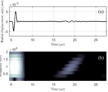
Fig.6shows the STFT spectrogram ofu(t)at transmitterTof model IM. In Fig.6, the first wave 192

packet (white-colored vertical shape) represented the transmitted ultrasonic wave traveling in the 193

longitudinal direction or path~s1(without geometric dispersion), whose amplitudes confirm our choice 194

(9)

on frequency range. The second wave packet (gray-colored tilted shape) represented the transmitted 195

ultrasonic wave traveling in the helical direction (with geometric dispersion) and coming back to 196

transmitter T. Due to the geometric dispersion in this FE simulation, ultrasonic waves at lower 197

frequencies (f <1 MHz) travel faster than the ones at higher frequencies (f >1 MHz). This explains 198

the tilted shape of the second wave packet. 199

Figure 6.Radial displacement and spectrogram of the intact steel rod model at transmitterT

Fig.7shows the STFT spectrograms ofu(t)at receiverRof all six models. In Fig.7, two wave 200

packets were observed within the time window of 4.5 - 27.5µs. The first wave packet centering at 8µs 201

represented the ultrasonic wave (vertical shape) propagating from transmitterTto receiverRalong 202

the longitudinal direction (z-axis). The second wave packet (tilted shape) represented the ultrasonic 203

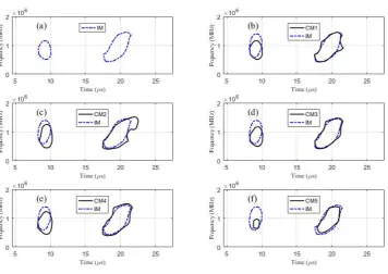
wave propagating along the helical direction or path~s2. Fig.8shows the contours at the half-power 204

level of the first wave packet in each spectrogram. In corroded steel rod models (CM1 CM5), higher 205

frequencies in the first wave packet were reduced due to smaller effective depth. In addition, shape of 206

the second wave packet changed due to the size change of surface rust, as shown in Fig.8. 207

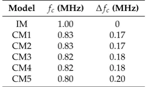
4.3. Surface rust detection 208

Detection of surface rust in a corroded steel rod model was accomplished by comparing its 209

centroid frequencyfcwith the one of an intact model (IM). Fig.9compares the half-power contours

210

of intact (model IM) and corroded (models CM1 CM5) FE models in individual STFT spectrogram at 211

receiverR. Center of the half-power contour of model IM was denoted by centroid frequency fc,i. For

212

five other corroded models, their centroid frequency was denoted by fc,cwith different values. After

213

findingfc,iandfc,c, their difference∆fcwas calculated and reported in Table3. Based on Eq. (1), the

214

(10)

10 of 18

Figure 7.Spectrogram of intact and corroded steel rod models at receiverR

Table 3.Centroid frequency (fc) of half-power contour for all models

Model fc(MHz) ∆fc(MHz)

IM 1.00 0

CM1 0.83 0.17

CM2 0.83 0.17

CM3 0.82 0.18

CM4 0.82 0.18

CM5 0.80 0.20

4.4. Surface rust localization 216

Eq. (3) was used to locate surface rust in our simulations. In view of the presence of geometric 217

dispersion inu(t), measuring TOF in the time domain became challenging. To avoid the problem of 218

chasing multiple frequencies at a time, the center frequency of transmitted ultrasonic wave in the STFT 219

spectrogram (i.e., 1 MHz in this paper) was chosen. 220

Fig.10shows the STFT spectrogram (at 1MHz) of model IM at receiverRto demonstrate how to 221

calculate the TOF of the scattered wave (t0₂) traveling through paths~s3and~s4. In Fig.10(a), the 1-MHz 222

curves on the STFT spectrogram of model IM and model CM1 were extracted. Timet1denoted the 223

TOF of the first wave packet and timet2the second wave packet for model IM. In Fig.10,t1andt2 224

were measured from the timet0when the ultrasonic wave was introduced at transmitterT; in this 225

paper,t0=6.13µs. Since the peak amplitude of the first wave packet was 9.01µs,t1= (9.01−6.13)µs 226

= 2.88µs. With traveling distances1being 10 mm, the wave velocityc1can be calculated by 227

c1=

s1

t1 (12)

⇒c1= 10

2.88 =3.47 mm/µs, (13)

(11)

Figure 8.Half-power contours in STFT spectrogram for six models at receiverR

This wave velocity can be compared with the theoretical surface wave velocity ct. ct can be

228

approximated by [21] 229

ct≈ 0.87

+1.2ν 1+ν

s

E

2ρ(1+ν) (14)

WithE= 210,000 MPa,ρ= 7,850 kg/m3, andν= 0.3, approximated theoreticalctvalue was found to be

230

3.03mm/µs. Consequently, theoretical TOFttfor the first wave packet was found to be

231

tt= s1 −zl

ct (15)

⇒tt=3.14µs (16)

wheres1 = distance from center of transmitterTto receiver R(mm) (= 10 mm) andzl = distance

232

from center of transmitterTto the edge of loading area atT(mm) (= 0.5 mm). An error of 8.2% was 233

obtained between the approximated theoreticalctvalue and numericalc1value. 234

235

A subtracted/differential 1-MHz curve (subtract model IM from model CM1) was generated 236

and shown in Fig.10(b) from where differential TOF values of the first wave packett0₁and of the 237

second packett0₂were determined to be 15.16−t0=9.03µs and 22.28−t0=22.28−6.13=16.15µs, 238

respectively. In our algorithm, differential TOF of the second wave packett₂0 was used for surface rust 239

localization. 240

From the differential 1-MHz curve in Fig.10(b), a propagation velocity model from literature 241

[17] for elastic waves on a cylindrical geometry was used. 242

c4(s4) =3.47−0.8348

p s4

(12)

12 of 18

Figure 9.Half-power contours of the first wave packet at receiverR

Figure 10.Spectrograms of model IM and model CM1 at 1 MHz

In all six FE models,p= 12.7π= 39.9 mm. From the Mercator projection shown in Fig.3, it is clear that 243

s4= q

(d+s5)2+p2 (18)

⇒s4= q

(s1−s3)2+p2 (19)

(13)

Withs1= 10 mm,p= 39.9 mm,c1= 3.47 mm/µs,a= 3.47,b=−0.8348, Eq. (5) could be written as 244

3.47h(10−s3)2+39.92 i

− t₂0 −3.47s3 q

(10−s3)2+39.92+155.58t02−33.31s3=0 (20) ⇒5871.27−

102.71− q

20371.8−240.8s3+12.04s23

s3+3.47s23

+

155.58−q1692.01−20s3+s23

t0₂=0 (21)

Eq. (21) provides the condition betweens3andt02. With differential TOFt02, surface rust locations3 245

can be found from Eq. (21). Since Eq. (21) cannot be solved analytically, the graphic method was 246

applied with its result shown in Fig.11. Eq. (21) represents a model for locating the surface rust in our 247

algorithm. Following the same procedure, 1-MHz curves of models CM2 and CM3 were generated

Figure 11.Relationship betweens3andt02

248

(similar to Fig.10(b) for model CM1) in order to determine different TOF for models CM2 and CM3. 249

For model CM2,t0₂was found by 22.51−t0=22.51−6.13=16.38µs. For model CM3,t₂0 was found 250

by 23.01−t0=23.01−6.13=16.88µs. Oncet0₂was found, Eq. (21) can be used for finding surface 251

rust locations3. 252

Estimated surface rust locations (s3) in corroded steel rod models was reported in Table4. 253

Table 4.Comparison between predicted and actual location and dimensions

Model Predicted (mm) Actual (mm) Error(%)

Location,s3 CM1 3.86 4 3.5

CM2 5.91 6 1.5

CM3 2.92 3 2.6

Length,d CM1 1.97 2 1.5

CM2 3.69 4 7.75

Width,w CM1 2.36 2.2 7.27

CM4 4.2 4.4 4.54

Thickness,h CM1 0.98 1 2

(14)

14 of 18

4.5. Surface rust quantification 254

For surface rust quantification, Eq. (8) was used to determine surface rust lengthdfor models 255

CM1 and CM2 by using measured timet0₁. Eq. (9) was applied to determine surface rust widthwfor 256

models CM1 and CM4 by using measured timet0₈. Eq. (11) was utilized to determine surface rust 257

depthhfor models CM1 and CM5 by using measured curvature _d2_U

1

d f2

. 258

For determining surface rust lengthdby using Eq. (8),s1= 10 mm and propagation velocity in steel 259

c1= 3.47 mm/µs (from Eq.(13)). Propagation velocity in rustcrwas calculated by 0.08454ct=0.257

260

mm/µs from [20]. Therefore, Eq. (8) became 261

d(t0₁) = 0.257(10)−0.257(3.47)t 0

1

3.47−0.257 (22)

⇒d(t01) =

2.57−0.892t0₁

3.213 (23)

For model CM1,t0₁was found by 16.10−t0=16.10−6.13=9.97µs. For model CM2,t0₁was found by 262

22.31−t0=22.31−6.13=16.18µs. With Eq. (23), estimated surface rust lengthdfor models CM1 263

and CM2 were reported 1.97 mm and 3.69 mm, respectively. 264

was applied to determine surface rust lengthdfor models CM1 and CM2. Withs3(from surface 265

rust localization) anddfound, surface rust widthwvalues for models CM1 and CM4 were determined 266

by solving Eq. (9) with measuredt8(TOF of the first wave wave packet as shown in Fig.12). 267

Figure 12.Time delay of the first wave packet

For surface rust widthwquantification, estimateds3andd were substituted into Eq. (9). For 268

example, in model CM1, Eq. (9) became 269

t83.47− q

3.862_{+ (}_w_/2₎2₋_1.97₋q₍₁₀₋_3.86₋_1.97₎2_{+ (}_w_/2₎2₌₀ ₍₂₄₎ wheret8was found by 9.11−t0=9.11−6.13=2.98µs. Surface rust widthwvalues for model CM1 270

was hence determined to be 2.36 mm. Similarly, 271

t83.47− q

3.912_{+ (}_w_/2₎2₋_1.98₋q₍₁₀₋_3.91₋_1.97₎2_{+ (}_w_/2₎2₌₀ ₍₂₅₎ was obtained for models CM4.t8was found by 9.31−t0=9.31−6.13=3.18µs in CM4. Predicted 272

wis 4.2 mm as shown in Table4. 273

(15)

At last, curvature values of the first wave packet for models IM (∂2U1

∂f2 =−4.22×10

5_{), CM1 (}∂2U1

∂f2 =

274

−5.12×105), and CM5 (∂2U1

∂f2 =−4.72×10

5_{) were calculated from Fig.}₁₃_{(a). These curvature values} 275

were modeled with surface rust depthhby Eq. (11) to obtain model parameterse=−1.1053×105and 276

g=−4.6818 (R2₌_{0.996). Therefore, Eq. (}₁₁_{) was written as} 277

h

∂2U1

∂f2

=−1.1053×105× ∂ 2_U

1

∂f2 −4.6818 (26)

Performance of proposed algorithm (Eqs. (23), (24), (25) and (26)) for surface rust quantification 278

was summarized in Table4.

Figure 13.Ridge of the first wave packets and their second-order derivatives

279

4.6. Findings 280

By conducting the FE analysis of ultrasonic wave propagation in intact and corroded steel rod 281

models, following research findings are obtained: (1) in the time domain, the first peak amplitude 282

(u1) is reduced due to the presence of a surface rust; (2) in the STFT spectrogram, shape of the second 283

wave packet in the spectrogram is tilted due to the geometric dispersion in ultrasonic waves; (3) the 284

first wave packet in corroded steel rod models suffered from high frequency components loss. This is 285

because that higher frequencies have smaller effective depths and are affected by surface rust more 286

than lower frequencies. As a result, non-zero centroid frequency reduction∆fcoccurs to corroded steel

287

rod models; (4) when measuring TOF from dispersive ultrasonic waves, single frequency is used on 288

the STFT spectrogram (e.g., 1 MHz in this paper); (5) ultrasonic wave propagation velocity on different 289

curved paths can be estimated by an empirical model described in Eq. (4); (6) six empirical equations 290

are proposed for detecting (Eq. (1)), locating (Eq. (21)) and quantifying (Eqs. (23), (24), (25) and (26)) 291

surface rust on a steel rod model. Based on aforementioned findings, a surface rust detection algorithm 292

(16)

16 of 18

Figure 14.Surface rust detection algorithm

5. Conclusion 294

This paper reports a finite element study of utilizing point-source generated ultrasonic waves for 295

detecting surface rust in steel rod models. Methods of detecting, locating and quantifying the surface 296

rust are achieved by using the STFT (short time Fourier transform) spectrogram of radial displacement 297

collected on the surface of corroded steel rod models. We have concluded the following. 298

• Presence of surface rust can be detected by the reduction of centroid frequency of the first wave 299

packet in the STFT spectrogram of corroded steel rod models. 300

• Location of surface rust is estimated by finding the difference in arrival time (TOF) between 301

helically propagating ultrasonic waves and scattered ultrasonic waves (due to surface rust). 302

• Length of surface rust can be predicted by calculating the difference in TOF between longitudinally 303

propagating ultrasonic waves of intact and corroded steel rod models. This difference in TOF is 304

related to the longitudinal dimension (length) of surface rust. 305

• Width of surface rust can be determined by calculating the difference in TOF of the first wave 306

packet between intact and corroded steel rods in the STFT spectrogram at a fixed frequency (e.g., 1 307

MHz in this paper). 308

• Thickness of surface rust can be estimated by utilizing the second-order derivative of the first wave 309

packet of corroded steel rod models. 310

(17)

In conclusion, this paper presents our finite element analysis of ultrasonic waves on intact and corroded 311

steel rod models for detecting, locating, and quantifying surface rust in a systematically approach. 312

While research result is obtained in several empirical equations, it is believed that our proposed 313

damage detection algorithm can be applied to other corrosion detection problems using distributed 314

photoacoustic fiber optic sensors on steel rods or steel rebars. 315

Acknowledgments: The authors would like to thank the National Science Foundation (NSF), Division of 316

Civil, Mechanical and Manufacturing Innovation (CMMI) for partially supporting this research through Grant 317

CMMI-1401369. 318

Author Contributions:Qixiang Tang and Tzuyang Yu conceived and designed the simulation; Qixiang Tang, Jie 319

Hu and Cong Du analyzed the data; Xingwei Wang and Tzuyang Yu contributed analysis tools; Qixiang Tang 320

drafted the manuscript. 321

Conflicts of Interest:The authors declare no conflict of interest. 322

323

1. Huston, D.Structural Sensing, Health Monitoring, and Performance Evaluation; 2010. 324

2. for Testing, A.S.; Materials. Metals Test Methods and Analytical Procedures.1999 Annual Book of ASTM 325

Standards1999,3. 326

3. Qixiang Tang, Tzuyang Yu, M.J. Finite element analysis for the damage detection of light pole structures. 327

Proc.SPIE2015,9437, 9437 – 9437 – 15. 328

4. Cheng, W. Pulsed Eddy Current Testing of Carbon Steel Pipes’ Wall-thinning Through Insulation and 329

Cladding. Journal of Nondestructive Evaluation2012,31, 215–224. 330

5. Wallbrink, C.; Wade, S.A.; Jones, R. The effect of size on the quantitative estimation of defect depth in steel 331

structures using lock-in thermography. Journal of Applied Physics2007,101, 104907. 332

6. Cook, D.; Berthelot, Y. Detection of small surface-breaking fatigue cracks in steel using scattering of 333

Rayleigh waves. NDT & E International2001,34, 483–492. 334

7. Resch, M.T.; Nelson, D.V. An ultrasonic method for measurement of size and opening behavior of small 335

fatigue cracks. Small-crack test methods. ASTM International,1992, pp. 169–196. 336

8. Rodríguez, G.; Casas, J.; Villalba, S. SHM by DOFS in civil engineering: a review. "Structural Monitoring 337

and Maintenance. Structural monitoring and maintenance2015,2. 338

9. Li, H.N.; Li, D.S.; Song, G.B. Recent applications of fiber optic sensors to health monitoring in civil 339

engineering. Engineering Structures2004,26, 1647 – 1657. 340

10. Du, C.; OwusuTwumasi, J.; Tang, Q.; Guo, X.; Zhou, J.; Yu, T.; Wang, X. All-Optical Photoacoustic Sensors 341

for Steel Rebar Corrosion Monitoring.Sensors2018. 342

11. Zou, X.; Chao, A.; Tian, Y.; Wu, N.; .; Yu, T.; Wang, X. A novel Fabry-Perot fiber optic temperature sensor 343

for early age hydration heat study in Portland cement concrete.Smart Structures and System2013,12. 344

12. Wu, N.; Zou, X.; Zhou, J.; Wang, X. Fiber optic ultrasound transmitters and their applications.Measurement 345

2016,79, 164–171. 346

13. Tang, Q.; Yu, T. Finite element simulation for damage detection of surface rust in steel rebars using elastic 347

waves. Proceedings of SPIE Vol. 98042016. 348

14. Sansalone, M.; Carino, N.J. Detecting Delaminations in Reinforced Concrete Slabs with and without 349

Asphalt Concrete Overlays Using the Impact-Echo Method.National Bureau of Standards Journal of Research 350

1987,Nov./Dec., 369–381. 351

15. Tang, Q.; Yu, T. Finite element simulation of ultrasonic waves in corroded reinforced concrete for early-stage 352

corrosion detection. Proc.SPIE2017,10169, 10169 – 10169 – 9. 353

16. Zhang, S.; Shen, W.; Li, D.; X.Zhang.; Chen, B. NONDESTRUCTIVE ULTRASONIC TESTING IN ROD 354

STRUCTURE WITH A NOVEL NUMERICAL LAPLACE BASED WAVELET FINITE ELEMENT METHOD. 355

Latin American Journal of Solids and Structures2018. 356

17. Tang, Q.; Twumasi, J.O.; Hu, J.; Wang, X.; Yu, T. Finite element simulation of photoacoustic fiber optic 357

sensors for surface corrosion detection on a steel rod. Proc.SPIE2018,10599, 10599 – 10599 – 13. 358

18. Dassault Systémes, 10 rue Marcel Dassault, CS 40501, 78946 Vélizy-Villacoublay Cedex-France.Abaqus/CAE 359

(18)

18 of 18

19. Liu, G.R.; Quek, S.S. A non-reflecting boundary for analyzing wave propagation using the finite element 361

method. Fn. Elem. in Anal. Des.2003,39, 403–417. 362

20. Bergmann, L. Ultrasonics and their Scientific and Technical Applications. Wiley, New York1948. 363

21. Viktorov, I. Rayleigh Waves and Lamb waves-Physical Theory and Application. New York: Plenum1967. 364