Performance Comparison of EMD based Noise Classification for different SNR using GMM and k-NN Classifiers

(1)

International Journal of Emerging Technology and Advanced Engineering

Website: www.ijetae.com (ISSN 2250-2459, ISO 9001:2008 Certified Journal, Volume 5, Issue 9, September 2015)

197

Performance Comparison of EMD based Noise

Classification for different SNR using GMM and k-NN

Classifiers

Sujay D. Mainkar

Assistant Professor,Dept. of Electronics and Telecommunication Engineering, Finolex Academy of Management & Technology, Ratnagiri, Maharashtra, India

Abstract— In today’s era of digital revolution, electronic systems in the context of audio communication typically perform transmission, playback, analysis and synthesis of audio signals. So, from the perspective of electronic system/product design for any of these purposes, noise influences must be carefully considered. Various types of noise and distortion can be characterized and number of techniques can be assisted in mitigating their effects, thus enhancing the quality and intelligibility of the speech signal. The first and foremost step towards this characterization is noise classification. In this concern, this paper addresses the issue of environmental background noise classification using Empirical Mode Decomposition (EMD). Instead of using an apriori choice of filters or basis functions to separate a frequency component, the EMD typically expands the time series into a set of functions defined by the signal itself; commonly known as Intrinsic Mode Functions (IMFs). These IMFs (and not the actual signal) are then used for feature extraction. This work suggests hybrid feature vectors for classification and proposes an optimized best suitable feature set for classification of different noisy environments with variation in signal-to-noise ratio (SNR) level. For classification, Maximum-Likelihood Gaussian Mixture Model (ML-GMM) and k-Nearest Neighbor (k-NN) classifiers are used. Utilization of this optimized feature set yields the maximum accuracy in multiclass noise classification irrespective of SNR variation.

Keywords— Empirical Mode Decomposition, Intrinsic Mode Function, k-Nearest Neighbor classifier, Maximum-Likelihood Gaussian Mixture Model.

I. INTRODUCTION

Audio segmentation and classification have vital applications in audio content analysis, information retrieval, modern man-machine interfaces and in entertainment and security tasks. In case of systems designed for any of such real world applications, accurate identification and efficient classification of background noise scenarios is a crucial step for robust audio recognition. There are several problems which noise imposes in audio processing.

To deal with practical noisy environments, it is important to have an idea about noise characteristics itself. Environmental background noise signals are usually divided into two classes: stationary and non-stationary noise signals. Fan noise is one of the examples of stationary noise, where statistical characteristics remain unchanged over time. Examples of non-stationary noise include vehicular traffic noise or crowd of people speaking in the background, etc., where statistical characteristics vary w.r.t. time. Such noise affects audio applications beyond just speech recognition. In [10], authors note that noise influences e.g. audio compression and hearing aids. They suggest noise classification as one solution to problems in these areas as well as for speech recognition. The fact that noise signals can be characterized by their evolvement over time and frequency motivates to consider correct temporal and spectral characteristics to obtain unique signature of corresponding source.

(2)

International Journal of Emerging Technology and Advanced Engineering

198 This literature review identified a need of system design for multiclass noisy environment discrimination with accuracy improvement using EMD to tackle the inherent non-stationarity of audio signal.

This paper put forwards unique, optimized, appropriate feature set to make a distinction between multiple classes of environmental background noise sources irrespective of speakers, their gender and utterances to understand the surrounding environment of the speaker. The remainder of this paper includes overview of EMD in section II. The basic idea behind proposed approach is discussed in section III. Section IV explains feature extraction and feature selection. The classification algorithms used are discussed in Section V. Section VI presents experimental

II. Empirical Mode Decomposition

The empirical mode decomposition (EMD) is a completely data-driven method for the analysis of nonlinear and non-stationary time series. Instead of using a pre-decided choice of filters or basis functions for separation of a frequency element, the EMD proceeds with the time series expansion into an ensemble of functions defined by the signal itself. This signal is then characterized by the summation of amplitude- and frequency-modulated elements. The key theme behind the EMD algorithm is a sifting process that expands the signal into a set of zero-mean, AM and FM constituents called intrinsic oscillatory modes or functions (IMFs). The entire sifting approach for extraction of these modes from a given noisy audio time series s(t) can be summarized as follows [8]:

1. make out all extrema of s(t);

2. interpolate between minima (resp. maxima) to get

two envelopes smin(t) (resp. smax(t));

3. compute the mean envelope

m(t) = [smax(t)+smin(t)]/2 and extract the residual d(t) = s(t) −m(t);

4. iterate on d(t) till this final can be treated as zero mean according to a stoppage condition.

Once this process is completed the resulting signal is considered as an IMF. The obtained intrinsic mode C1 is extracted from s(t) and steps (1) – (4) are repeated to obtain the second mode C2. This sifting process continues until the last mode shows no apparent variation. At the end of the sifting process, the original signal is decomposed in a finite number of modes as s(t) = r(t) +Σi Ci(t), where r(t) stands for a residual trend, and the intrinsic modes Ci(t)s are nearly orthogonal to each other [8].

An oscillation must verify two criteria to be considered as an IMF:

1. the mean envelope defined through the local

maxima and the local minima is zero at any time; 2. the number of extrema and thus the number of

zero-crossings are equal or they differ at most by one.

III. PROPOSED APPROACH

The time-frequency analysis of input noisy audio signal with inherent non-stationarity is possible through proper front-end processing. In the present methodology, initially, the silence period is removed from the noisy audio clip under test. The remaining noisy audio stream is then decomposed into frames with frame period of 50ms and overlap period of 25ms. This frame overlapping guarantees that audio features occurring at a discontinuity are at least considered whole in the subsequent overlapped frame. These frames are then decomposed into number of IMFs. From these IMFs, different temporal and spectral features are extracted to form hybrid feature vectors as described in section IV below. Finally, classification is done using

Maximum Likelihood Gaussian Mixture Model

(ML-GMM) and k-Nearest Neighbor (k-NN) classifiers, followed by performance evaluation, so as to conclude with unique optimized feature set which is best suitable for discrimination of various noisy environments irrespective of variation in SNR level.

IV. FEATURE EXTRACTION AND FEATURE SELECTION

A. Feature Extraction

For capturing the audio data characteristics, the feature

extraction is an indispensable processing step in multiclass audio classification tasks. The goal is to extract that set of features from the noisy audio stream of interest which is capable of conveying maximum information regarding desired characteristics of the original signal. Feature extraction involves the analysis of the noisy input audio stream. The feature extraction methods can be categorized into temporal analysis and spectral analysis approaches. Temporal analysis uses the time-domain waveform of the audio signal itself for analysis.Spectral analysis utilizes frequency domain representation of the audio signal for analysis. All audio features are extracted from IMFs generated by splitting the input signal into a series of analysis windows or frames, and computing one feature value for each of the windows.

B. Feature Selection

(3)

International Journal of Emerging Technology and Advanced Engineering

199 Further, these features determine the dimensionality in the feature space. Thus, it is important to opt for minimum number of features that not only keeps agreement with the accurateness and the level of performance but also reduces the computational costs. Therefore, a selected feature must have the following properties:

1. Robustness to irrelevancies: This refers to the requirement that any good quality feature should be able to tolerate irrelevancies such as noise, bandwidth or the amplitude scaling of the signal. Further, it also depends on the discrimination system to consider such variations as irrelevant to achieve better classification across a wide range of audio formats.

2. Discrimination Capability: The rationale behind feature selection is to achieve discrimination among different classes of audio patterns. Therefore a feature must take roughly similar values within the same class but must isolate dissimilar values into distinct classes.

3. Uncorrelatedness towards other features: It is very important that there are no redundancies in the feature space. Each newly chosen feature must present entirely different information about the signal as possible [9].

In this work, we have selected Short Time Autocorrelation Function (ACF), Short Time Energy (STE) and Zero Crossing Rate (ZCR) as temporal features and Spectral Centroid (SC), Spectral Roll off (SR) and Spectral Flux (SF) as spectral features [3]. Further, we also have chosen Mel Frequency Cepstral Coefficients (MFCC) as one of the feature. Further, here, we do experimentations by using hybrid feature vectors formed by combining multiple features for all frames of first IMF.

V. CLASSIFICATION

For the classification purpose, we have used k-Nearest Neighbor (k-NN) classifier which is an instance based classifier and Maximum-Likelihood Gaussian Mixture Model (ML-GMM) classifier.

A. k-Nearest Neighbor Classifier

The k-NN algorithm (k-Nearest Neighbor) can be classed as a nonlinear non-parametric classification method. This algorithm is based on very simple principle that similar data are close to each other in the searching or data space. In other words, for every object from test data set of k objects the k-NN finds the training data that are closest to the test object (nearest neighbors). The label assignment is usually based on the rule of majority voting, e.g. the most frequent class from the k nearest neighbors for given test object determines the class where this object

should belong. A value of k dictates a number of closest objects from training data that are taking into account at the label decision. If the value is too small, then the result can be sensitive to noise points. If it is too large, then the neighborhood may contain lots of points from other classes [13].

Example of k-value impact to classification result is shown in Fig. 1, where, k-NN classifier classifies two dimensional data into two classes. First circle represents a region with three neighbors are involved into making decision where orange point is belonging. In this case k value is set to three (k = 3) and classified data/point belongs to ‗red‘ class. Second circle represents six neighbors (k = 6) considered in classification task. In the second case, the classification result is an opposite and unknown data/point belongs to ‗blue‘ class [11].

Fig.1. Illustrative Example of k-NN Classification [11]

Besides a k value, the distance metric is important to the k-NN algorithm. As can be clearly seen, the distance metric represents the measure of data similarity. The choice of particular distance metric usually depends on the given classification problem. Regardless simplicity of k-NN, this method is well suitable for multi-modal classes, very flexible and fits into top 10 data mining algorithms [12].

B. Gaussian Mixture Model Classifier

(4)

International Journal of Emerging Technology and Advanced Engineering

[image:4.612.107.228.124.232.2]

200 Fig.2. Illustrative Example of modeling 2-dimensional data using

4-Gaussian mixtures [11]

The identification assignment is maximum likelihood classifier. The main task of the system is to make a decision if input noisy audio belongs to one of the set of noisy environments, which are represented by its models. This decision is based on computation of maximum posterior probability for input feature vector [11].

VI. EXPERIMENTAL RESULTS

A. Audio Database

For our experimentation purpose, we have used NOIZEUS database. NOIZEUS is a noisy speech corpus recorded in laboratory for comparison of various algorithms related to speech enhancement among research groups. But, we used it for identification and classification of different real-world noises due to following reasons:

1. High quality: these recordings are of high quality

and were made in sound-proof chamber,

2. Versatility: it includes eight different types of noises from AURORA database by [13] which corrupt the original recordings at four different SNR levels,

3.

Gender Variation: recordings by six different

speakers that includes three male voices and three female voices,

4.

Standardization: it utilizes the IEEE sentence database that contains phonetically-balanced sentences with relatively low word-context predictability,

5. Availability: the database is available to

researchers free of cost [14].

The system is used for multiclass classification of 4 representative noisy environment types namely-babble, car, exhibition hall and train noise with variation in SNR level (0dB, 5dB and 10dB). This work uses 9600 frames of audio streams for experimentation.

Results of different experimentations performed under varying conditions are presented here.

B. Comparison of results and Discussion

1. Evaluation of feature-set effectiveness:

For evaluation feature-effectiveness of each feature set, we have experimented for 17 different varieties of hybrid feature vectors comprising of combination of multiple features corresponding to first IMF, for all the frames of all 30 samples associated with 4 noisy environments, for 3 different SNR levels (0dB, 5dB and 10dB) using both ML-GMM and k-NN (k=3,5,7) as presented in Table I.

TABLE I: List of hybrid feature sets used for experimentation

Set No. Hybrid Feature Set

1 ZCR-SF 2 ZCR-SF-MFCC 3 SF-MFCC 4 ZCR-MFCC 5 STE-MFCC 6 STE-ZCR 7 STE-SF 8 ZCR-SF-MFCC

9 ZCR-STE-MFCC

10 STE-SF-MFCC 11 SC-SF-SR 12 SR-STE-SF-MFCC 13 SR-STE-SC-MFCC 14 ZCR-STE-SF-MFCC 15 ZCR-STE-SF-SC 16 ZCR-STE-SF-SR 17 SC-STE-SF-SR

[image:4.612.358.529.308.573.2]

(5)

International Journal of Emerging Technology and Advanced Engineering

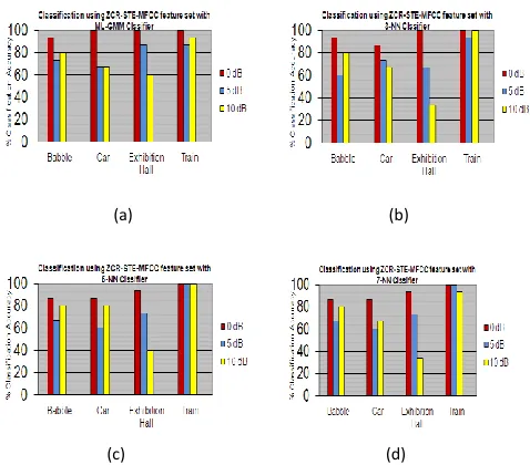
201 2. Comparison of classifier performance with variation in SNR level:

Fig. 3 highlights that, irrespective of change in SNR levels, ML-GMM classifier shows better results for all 4 types of noises. It can also be noted that, classification accuracy for babble noise almost remains unchanged, irrespective of variation in type of classifier used for classification. Further, classification accuracy for train noise is better for all classifiers considered here.

(a) (b)

[image:5.612.342.536.258.370.2]

(c) (d)

Fig.3. Comparison of classifier performance with ZCR-STE-MFCC for first IMF with variation in SNR level using (a) ML-GMM classifier (b) 3-NN classifier (c) 5-NN classifier (d) 7-NN classifier

3. Confusion Matrix:

The accuracy of the discrimination technique is the capability of the approach to correctly identify the class of a randomly selected data instance. If the test data has a total of N objects and during testing phase, suppose we find that n of the N objects are correctly discriminated, then error rate may be defined as: Error Rate = n/N. But, such an error rate is only a rough estimate of true error rate and it is expected to be a good estimate only if the number of test data N is large enough and representative of the population. A method of estimation of the error rateis treated asbiased if it either tends to underestimate the error or tends to overestimate it.

[image:5.612.47.286.259.469.2]

That is why, there lies need of using unbiased methods. Thus, sometimes for representing the result of testing, the ‗confusion matrix‘ is utilized as illustrated in Table II. The advantage of using this matrix is that, it not only tells us how many samples got misclassified but also exactly where misclassifications occurred. For example in Table II, we can see that only one sample that belonged to babble noise class got misclassified to car noise.

TABLE II: A confusion matrix (%) for 4 noise classes at 0dB SNR using ML-GMM classifier

(B: Babble; C: Car; E: Exhibition Hall; T: Train)

We can describe the terminologies ‗false positive‘ (FP) and ‗False Negative‘ (FN) by means of Table II. False positive cases are those that did not belong to a class but were allocated to it. For example, there is 1 false positive for car noise class and other three classes do not have any false positives. False negative on the other hand are cases that belong to a class but were not allocated to it. For example, there is 1 false negative for babble noise class and nothing for other categories. Further, the total number of correctly classified samples are denoted by ‗true positive‘ (TP) and ‗true negative‘ (TN) is the totality of samples discriminated to a category actually they are not belonging to. Such detailed analysis is carried out for 12 different confusion matrices corresponding to ML-GMM and k-NN (k=3,5,7) classifiers and 3 SNR levels (0dB, 5dB, 10dB) for all 4 noise classes. The results of this analysis are summarized in Table III.

4. Comparison of performance using different measures:

The evaluations discussed so far help us in evaluating the cost of making wrong decisions in turn leading to incorrect classification by the system under consideration, as summarized in Table III here:

T

ru

e

C

la

ss

Predicted Class

Class B C E T

B 93.33 6.67 0 0

C 0 100 0 0

E 0 0 100 0

(6)

International Journal of Emerging Technology and Advanced Engineering

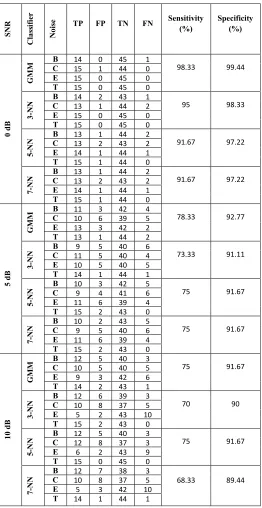
[image:6.612.40.302.172.680.2]

202 TABLE III: Summary of different metrics used for performance

comparison SN R C la ss if ie r N oi

se TP FP TN FN Sensitivity

(%) Specificity (%) 0 dB GM

M B C 14 15 0 1 45 44 1 0 98.33 99.44

E 15 0 45 0

T 15 0 45 0

3-NN

B 14 2 43 1

95 98.33

C 13 1 44 2

E 15 0 45 0

T 15 0 45 0

5-NN

B 13 1 44 2

91.67 97.22

C 13 2 43 2

E 14 1 44 1

T 15 1 44 0

7-NN

B 13 1 44 2

91.67 97.22

C 13 2 43 2

E 14 1 44 1

T 15 1 44 0

5

dB

GM

M B C 11 10 3 6 42 39 4 5 78.33 92.77

E 13 3 42 2

T 13 1 44 2

3-NN

B 9 5 40 6

73.33 91.11

C 11 5 40 4

E 10 5 40 5

T 14 1 44 1

5-NN

B 10 3 42 5

75 91.67

C 9 4 41 6

E 11 6 39 4

T 15 2 43 0

7-NN

B 10 2 43 5

75 91.67

C 9 5 40 6

E 11 6 39 4

T 15 2 43 0

10

d

B

GM

M B C 12 10 5 5 40 40 3 5 75 91.67

E 9 3 42 6

T 14 2 43 1

3-NN

B 12 6 39 3

70 90

C 10 8 37 5

E 5 2 43 10

T 15 2 43 0

5-NN

B 12 5 40 3

75 91.67

C 12 8 37 3

E 6 2 43 9

T 15 0 45 0

7-NN

B 12 7 38 3

68.33 89.44

C 10 8 37 5

E 5 3 42 10

T 14 1 44 1

(B: Babble; C: Car; E: Exhibition Hall; T: Train)

In the Table III, two performance metric terms namely – ―sensitivity‖ and ―specificity‖ are used. Sensitivity relates to the test's ability to identify a condition correctly. Mathematically, this can be expressed as:

TP

Sensitivity

TP FN





On the other hand, specificity is associated with the ability of test samples to leave out a condition accurately. Mathematically, this can also be written as:

TN

Specificity

TN FP





Table III illustrates that, the value of sensitivity decreases considerably with respect to change in SNR from 0 dB to 10 dB but percentage of specificity remains fairly good, irrespective of variation in SNR. The reason is quite obvious as sensitivity is a function of TP and TP reduces with rise in SNR level because 0 dB refers to maximum noisy condition (signal power = noise power) whereas, 10 dB implies least noisy case under consideration (Signal power = 10 times noise power). This work is focused on noise classification and modeling here yields maximum sensitivity for maximum noisy condition.

VII. CONCLUSION

In this paper, we have presented and compared in detail ML-GMM based and k-NN (k=3,5,7) based approaches for classification of audio streams with 0 dB, 5 dB and 10 dB SNR levels. An audio clip is classified into one of the four classes: babble, car, exhibition hall and train. This work also proposed 17 different hybrid feature sets for the representation of audio streams and identified the best suited one. The effectiveness of these features is evaluated in experiments. Further, experimental evaluations show that the ML-GMM classifier achieves high accuracy in noisy audio classification, irrespective of variation in SNR levels. Moreover, overall system performance is judged in terms of sensitivity and specificity and found that, sensitivity reduces considerably with respect to change in SNR from 0 dB to 10 dB but percentage of specificity remains fairly good.

As for future track, we will work out with different

(7)

International Journal of Emerging Technology and Advanced Engineering

203 REFERENCES

[1] N. Nitanda, M. Haseyama, and H. Kitajima, ―Accurate audio segment classification using feature extraction matrix,‖ Proc.

ICASSP, 2005.

[2] M. A. Sobreira- Seoane, A. R. Moleras and J. L. A. Castro, ―Automatic classification of traffic noise‖, Proc. Acoustics‘08, Paris, June 29 – July 4, 2008.

[3] George Tzanetakis, Perry Cook, ―Musical Genre Classification of Audio Signals‖, IEEE Transactions on Speech And Audio

Processing, Vol.10, No. 5, July 2002.

[4] B. Han and E. Hwang, ―Environmental sound classification based on feature collaboration‖, Proc. ICME, 2009.

[5] Thiruvengatanadhan Ramalingam and P. Dhanalakshmi, ―Speech/Music classification using wavelet based feature extraction techniques‖, Journal of Computer Science 10(1): 34-44, 2014. [6] S.P.Mahajan, Jyotsana Sahu, M.S.Sutaone, V.K.Kokate, ―Improving

Performance of Multiclass Audio Classification using SVM‖, CIIT International Journal of Data mining and Knowledge Engineering, Volume 2,No 5,pp.95-103,ISSN 0974-9683, May 2010.

[7] Deepak Jhanwar, Kamlesh K. Sharma and S. G. Modani, ―Classification of Environmental Background Noise Sources Using Hilbert-Huang Transform‖, International Journal of Signal Processing Systems Vol. 1, No. 1 June 2013.

[8] N. E. Huang, Z. Shen, S. R. Long, M. L. Wu, H. H. Shih, Q. Zheng, N. C. Yen, C. C. Tung and H. H. Liu, ―The Empirical Mode Decomposition and Hilbert spectrum for nonlinear and non-stationary time series analysis,‖ Proc. Roy. Soc. London A, vol. 454,

pp. 903-995, 1998.

[9] J. J. Burred and A. Lerch, Hierarchical Automatic Audio Signal Classification, Journal of Audio Engg. Soc., Vol. 52, pp. 724-739, July/August 2004.

[10] Sunita Maithani and Richa Tyagi. Noise characterization and classification for background estimation, IEEE-International Conference on Signal processing, Communications and Networking, pages 208–213, Chennai, India, 2008.

[11] Hric, M.; Chmulik, M.; Jarina, R.; "Comparision of Selected Classification Methods in Automatic Speaker identification," COMMUNICATIONS Scientific Letters of the University of Zilina, vol. 13, 2011.

[12] X. Wu, Vipin K., The Top 10 Algorithms in Data Mining, Chapman & Hall/CRC, 2009.